• Federal Highway Administration >
• Publications >
• Research Publications >
• 05083 >
• Appendh.Cfm
• Appendix H. Live-Load Vibration Substudy

Previous | Table of Contents | Next

Appendix H. Live-Load Vibration Substudy

INTRODUCTION

This live-load vibration substudy was carried out to assess the amount of vibration which is caused by live loading. To address this problem, a computer model of a cable-stayed bridge was used to model the dynamic effects of a moving train load. The vibrations of an individual set of cables were analyzed in detail. The cable tensions, displacements, and anchorage rotations obtained from the dynamic time history analysis were compared with the results obtained from influence line calculation which are normally carried out during design. The engineering analyses were performed using in-house programs for nonlinear analysis (CAMIL) and live-load analysis (MELL).

Example Bridge: Rama 8 Bridge in Bangkok, Thailand

The RAMA 8 Bridge, shown in figure 151, is a cable-stayed bridge over the Chao Phraya River in Bangkok, Thailand. The bridge has been designed to carry four lanes of vehicle traffic and two pedestrian sidewalks on the main span and the back spans, and six lanes of traffic on the anchor span.

Total length of the main bridge is 475 m (1,558 ft): the main span is 300 m (984 ft), the two backspans are 2 × 50 = 100 m (328 ft), and the anchor span is 75 m (246 ft). The 160-m (525-ft)- high tower is a reinforced concrete inverted Y-type structure. There are two inclined cable stay planes with 28 cables each for the main span and one cable stay plane with 28 cables for the anchor span. Cable stays are BBR Cona stays, consisting of seven-wire parallel strands, greased and sheathed. The main span superstructure has an effective depth of 2 m (6.6 ft) and consists of a 29.7-m (97.4-ft)-wide deck which is made composite with two steel-edge girders. The backspan girder is a continuous posttensioned 2.5-m (8.2-ft)-deep concrete box girder.

Figure 151. Photo. RAMA 8 bridge (artistic rendering).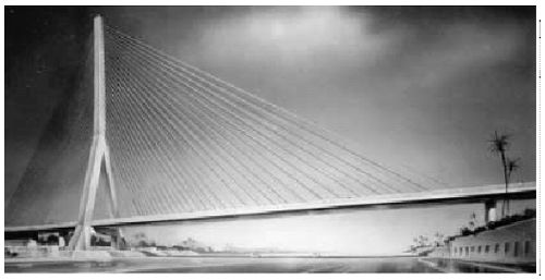

Rama 8 Bridge Computer Model

The RAMA 8 Bridge computer model, shown in figure 152, was created to represent the global behavior of the bridge under static and dynamic loads. The complete bridge, with two approach spans, was modeled in three dimensions. The model has 1,014 beam elements and 84 cable elements.

Figure 152. Drawing. RAMA 8 Bridge computer model: XY, YZ, and ZX views.

FREE-VIBRATION ANALYSIS

Description of Example Cable

The cable chosen to illustrate the effects of live loading on cable dynamics is the third longest cable of the main span of the RAMA 8 bridge—main span cable M26. The longest cable (M28) was not chosen as it is close to the support and would not be excited as much by moving loads.

The example cable M26 has the following properties:

Cable geometry is defined with the following end points:

• Cable anchor points at the tower: x = 1.247 m, y = 1.405 m, z = 184.326 m
• Cable anchor points at the deck: x = 268.578 m, y = 11.447 m, z = 48.293 m
• Cable angles in the cable plane (to the horizontal plane):
  At deck: α = 25.824°
  At tower: α = 28.068°
• Cable angle in horizontal plane: β = 2.151° (to the x-axis)

where x is the longitudinal coordinate measured from the centerline of the tower towards pier P39, and y is the transverse coordinate measured from the bridge centerline-positive upstream (see figure 152).

Single Cable Dynamics–Free Vibration

Theoretical solutions are based on the assumption that the cable is inextensible. (See appendix G for a brief discussion of the cable vibration theory.) However, the numerical analyses, which were carried out using cable elements, modeled a real (extensible) cable. These results were then compared to the theoretical (inextensible) cable.

Extensible Cable Model

To capture the dynamic behavior of a single cable it is necessary to introduce additional degrees of freedom along the cable. (This is not typically required when the global dynamics of the bridge are evaluated.) Three computer models were built to simulate the behavior of the cable as an element independent of the structure (i.e., tower and the deck) and to investigate the convergence of the results. In these models, cable M26 was divided in 2, 10, and 20 segments of equal length. Figure 153 shows nodes and cable elements of the cable stay M26 in the 10- segment model. The cable was discretized in a similar manner in the 2- and 20-segment models.

Figure 153. Chart. Independent cable M26 discretization 10-segment model: XZ view.

Coordinates of cable nodes were defined using the cable parameters and the catenary equations for this cable (see also figure 154), as shown in equations 137 and 138:

(137)

(138)

where:

(139)

and

(140)

Figure 154. Chart. Cable catenary.

Only the cable end points are fixed, so the cable can vibrate spatially, not only in its plane. Free independent cable vibration periods obtained by analysis are shown in table 19. Some typical cable modes for the 20-segment model are shown in figure 155. All of these plots contain XY, YZ, and XZ views of the cable and its mode shape.

Figure 155. Chart. Cable modes: XZ, YZ, and XY views (as defined in figure 152).

It can be seen that the cable vibrates only in its plane or perpendicular to its plane (out-of-plane vibration) for all modes. The vibration periods and frequencies are in fairly good agreement with theoretical values, and the error is 3.9 percent for the first mode and 5.2 percent for the third mode, for the 20-segment model.

The differences in natural frequencies are caused by several factors:

• The formula used to obtain the theoretical value is derived only for out-of-plane vibrations of a horizontal cable with small sag, neglecting the influence of cable extensibility due to existing tension in the cable, which is considered to be constant.
• The cable chosen is not horizontal, with varying tensile force along the cable (2 percent difference in tension between top and bottom), and is subjected to extension due to the tensile force.

The software used for analysis also accounts for cable extensibility, which is the most important factor causing differences in results.

It can also be seen that for symmetric modes, especially mode 1 (which carries most of the energy), the frequency for the in-plane mode is lower than for the out-of-plane mode. This is due to the fact that additional tension in the cable is generated in symmetric modes, so the cable becomes stiffer and, hence, the frequency increases.⁽⁵⁹⁾ The magnitude of the difference between the out-of-plane and in-plane frequencies depends on many parameters, but the most influential factors are the magnitude of the cable tensile force and cable stiffness parameters (area and unstressed length).

Inextensible Cable

An inextensible cable model was used to achieve results closer to the theoretical values. The same model was used as for previous analyses except that the cable area was increased to 100,000 mm² (160 inches²). This caused the cable to be very stiff axially. Since no other parameters were changed, a high tensile force (T = 58,252 kN (13,106,700 lbf) was induced in the cable. To lower the force to the previous level, the cable unstressed length was increased to USL = 300.016 m (984.05 ft). This resulted in an average tension of T = 2,776 kN (624,600 lbf), which was close to the value previously used (T = 2,773 kN (623,925 lbf)). With these parameters, free vibration periods obtained are given in table 20.

The agreement between analysis values and theoretical values for out-of-plane vibrations is now excellent, with errors well below 1 percent.

Mode shapes are very similar to those shown in the subsection “Extensible Cable Model” except for in-plane mode 1, which is shown in figure 156. The period for this mode is much smaller (27 percent) than for the out-of-plane mode because of a large increase in induced cable tension. Because of the great stiffness of the cable, any small differential movement induces large tensile orces in the cable, which has influence on the frequency increase. This effect is seen only in symmetric modes and diminishes as the mode number is increased.

The mode shape, as seen in figure 156, does not have a sine shape. It can be seen that inflection points exist in the vicinity of cable endpoints.⁽⁵⁹⁾

Figure 156. Chart. Inextensible cable mode 1, in-plane: XY, YX, and XZ views.

Cables Modeled as Part of the Structure

Modeling

Three computer models were again used to check the convergence of dynamic behavior of cable elements connected to the bridge deck and the tower. In these models, cable M26 was, as with the independent cable, divided in 2, 10, and 20 segments of equal length. Both the upstream and downstream cables in the main span were modeled. Figures 157 and 158 show nodes and cable elements of cable stay M26 for the 10-segment model. The cable was discretized in a similar manner in the two-segment and the 20-segment model. Coordinates of cable nodes were defined using the catenary equation for this cable.

Figure 157. Drawing. Cable M26 discretization: 10-segment model, isometric view. Only cables M26 are shown. Other cables not shown for clarity.

Figure 158. Drawing. Cable M26 discretization: 10-segment model, XZ view. Other cables not shown for clarity.

Global Bridge Modes

The global modes of the bridge are shown in figures 159 and 160. The fundamental vertical, longitudinal, and transverse modes are shown in figure 159. The second vertical and transverse and functional deck torsional modes are shown in figure 160. It can be seen from these modes that the cables participate in these global modes. (Note: Since only the M26 cables were discretized in detail, the vibration of the other cables is not visible). Therefore, the global modes will be reflected in the cable’s response to the moving load.

Cable Modes

The natural vibration periods for the cables obtained from the analysis are given in table 21 and the mode shapes are shown in figures 161 to 163.

Because the cables now form part of the overall structure, the modes of the two identical M26 cables become weakly coupled. This means the cables either move in-phase or out-of-phase with respect to each other and thus the number of modes is doubled. It can be seen that pure in-plane and pure out-of-plane vibration of the cable is present only for the first fundamental cable mode. Higher modes are spatial (i.e., they involve complicated 3D motions), which is a further consequence of the interaction with the deck and tower. However, the vibration periods and frequencies are in good agreement with theoretical values, especially for the 10-segment and 20- segment cable models, for which the error in period for the first mode is less than 1 percent.

Figure 159. Chart. Fundamental bridge modes.

Figure 160. Chart. Additional bridge modes.

Figure 161. Chart. Four first modes of the cables: XY, YZ, and XZ views.

Figure 162. Chart. Four second modes of the cables: XY, YZ, and XZ views.

Figure 163. Chart. Four third modes of the cables: XY, YZ, and XZ views.

STATIC LIVE-LOAD ANALYSIS

Static live-load analyses were performed using the influence line based program MELL and the train passage option of the bridge analysis program CAMIL, neglecting any dynamic properties of the train. For the latter program, the train live load was considered as a series of concentrated loads moving along the bridge over selected nodes. The train was treated as a static load and bridge dynamics were ignored so the bridge only responded statically to the train loading.

The live load used was a five-car transit train. (A transit train was used because it represents a large moving load. Furthermore, the dynamic model for a transit train was used because it is more readily defined than a highway truck model, for which there are a large number of dynamic configurations). Each car weighed 369.5 kN (83,138 lbf), thus the total weight of the train was 1,847.5 kN (4,156,875 lbf). The train load was applied along the main span girder line. The dynamic allowance was taken as zero. Influence line analyses were performed using 200 (design accuracy) and 5,000 (academic accuracy} steps (iterations) in the longitudinal positioning of the live load along the influence line to find the minimum and maximum effects due to live load. Computed results were tabulated for nodal deformations, girder member effects, and main span cable forces and rotations at several locations, as identified in figure 164.

Figure 164. Chart. Nodes, members, and cables for comparison of results.

Displacements

Vertical displacement results are summarized in table 22. Differences in results for displacements from analyses using 200 and 5,000 calculation steps are practically nil. The differences between MELL’s results and CAMIL’s static train results are a maximum of 2.5 percent.

Bending Moments

Bending moment results are summarized in table 23. Differences in results for bending moments from analyses using 200 and 5,000 calculation steps are a maximum of 0.45 percent. The differences between MELL’s results and CAMIL’s static train results are a maximum of 3.4 percent.

Table 23. Bending moments due to live load.

Bending Moment (Strong Plane) (kNm)
		Influence Line Analysis/Steps		Train Static
	Member	200	5,000
	1,071	2,845	2,849	2,900
	1,075	2,610	2,646	2,680
	1,141	3,984	3,998	4,010
	1,145	3,866	3,883	3,920
	1,211	4,564	4,579	4,650
	1,215	4,491	4,511	4,610
	1,071	–2,452	–2,452	–2,470
	1,075	–2,549	–2,554	–2,570
	1,141	–3,261	–3,261	–3,320
	1,145	–3,375	–3,376	–3,430
	1,211	–1,625	–1,625	–1,570
	1,215	–1,295	–1,298	–1,290

1kNm=738 lbf-ft.

Cable Tensions

Cable force results summarized are in table 24. Differences in results for cable forces from analyses using 200 and 5,000 calculation steps are very small. The differences between MELL’s results and CAMIL’s static train results are a maximum of 0.55 percent.

Table 24. Cable forces due to live load.

Max Cable Force T1 (kN)
		Influence Line Analysis/Steps		Train Static
	Member	200	5,000
	M7	269	269	270
	M14	322	322	324
	M21	391	391	393
	M26	230	230	230
	M7	–24	–24	–24
	M14	–14	–14	–14
	M21	–8	–8	–7
	M26	–20	–20	–20

1 kN = 225 lbf.

Cable End Rotations

Cable end rotations, deck rotations, and the relative differences between the two are summarized in table 24. Differences in results from analyses using 200 and 5,000 calculation steps are again practically zero. The differences in cable deck and relative rotations between MELL and CAMIL results are also very small.

Some differences exist between MELL’s results and CAMIL’s static train results for cable end rotations. The cable end rotations are not directly generated by the programs. Therefore they have to be computed according to the formula:

(141)

where:

Since the cable end rotations are very small numbers, any small difference in calculating the V_LL and H_LL using MELL and CAMIL leads to small numbers that are close to each other in actual value but very different if expressed in percentages.

DYNAMIC LIVE-LOAD ANALYSIS

Dynamic live-load analyses were performed using the train option in the bridge analysis program. In this option, the train is considered as a dynamic moving load with its appropriate stiffness and damping parameters. Each train car is modeled as a mass (consisting of the car mass and the passengers mass) supported by springs and dampers that are fixed to bogies. Each bogie has its own unsprung mass and is supported by two axles. The axles transfer train load to nodes specified in the input file (usually main girder nodes). The dynamic response of the bridge due to the dynamic train loading was calculated using the Newmark’s direct integration procedure.

Damping

For the structure’s damping matrix calculation, the Rayleigh damping coefficients α and β were determined using frequencies of the 1^st and the 15^th bridge natural mode. The damping ratio at those two frequencies was set at 0.75 percent of critical. The variation of damping with frequency corresponding to the above criteria is shown with a heavily solid line in figure 165. This figure also shows the damping distributions which would have resulted from picking 1^st and 2^nd or the 1^st and 22^nd modes to define the damping. The figure clearly indicates that for the frequency range of interest an acceptable damping distribution is achieved (see equations 142 through 146).

(142)

(143)

(144)

(145)

and

(146)

Figure 165. Graph. RAMA 8 Bridge model damping versus frequency.

Results for Train Speed of 80 km/h (50 mi/h)

The results obtained for a train speed of 80 km/h (50 mi/h) are discussed in this section. The results for other train speeds are outside the scope of this study.

Deck Displacement Time Histories

The displacement time histories for both the static and dynamic load cases for node 427 (near the 3/4 span location of the main span) are shown in figure 166. (This load case ignores dynamic effects and only captures the effect of the moving load position.) This figure shows that the dynamic displacement was only slightly larger than the static displacement. Furthermore, the bridge deck oscillations, which occurred after the train had left the bridge (the train has completely left the bridge at 20 s into the time history), were small in comparison to the static response. This figure also displays the velocity and acceleration records corresponding to the displacement time history.

The velocity record shows some higher frequency oscillations in the 15-s range which correspond to the individual cars leaving the bridge. As the first set of bogies left the bridge by moving across the pin joint at the end of the main span, the slope discontinuity setup pitching motions that were fed back to the structure via the second set of bogies. This phenomena can also be observed in the acceleration time history, which shows a baseline acceleration corresponding to the static displacement and the accelerations due to the train superimposed until the train left the bridge.

Figure 166. Graph. Vertical displacements, velocities, and accelerations of node 427 versus time (train speed = 80 km/h (50 mi/h)).

Deck Girder Bending Moment Time History

The static and dynamic bending moment time histories for a deck girder member are shown in figure 167. This figure shows that there was very little amplification due to dynamic effects. Both the static and dynamic time histories show oscillations in the maximum bending moment because of the passing of individual train cars. The dynamic moments after the train had left the bridge are negligible when compared to the static moments.

Figure 167. Graph. Member 1211: Bending moment versus time (train speed = 80 km/h (50 mi/h)).

Cable Tension Time Histories

The total cable force versus time diagram for a train speed of 80 km/h (50 mi/h) is shown in figure 168. The dynamic time history has the same shape as the static time history, but there are slightly larger maxima and minima due to dynamic effects. This figure also shows the maximum and minimum obtained from the influence line analysis.

Figure 168. Graph. Cable M26, tension versus time (train speed = 80 km/h (50 mi/h)).

The difference in cable tension for cable M26 between the dynamic train load case and static train load case, for train speed 80 km/h (50 mi/h), is shown in figure 169.

The tension spectrum for cable M26 is shown in figure 170. This spectrum was generated from the part of the cable tension time history which corresponds to the time after the train has crossed the bridge (i.e., to the cable tension time history due to free bridge vibration, 20 s of elapsed time).

The two dominant peaks in the cable tension spectrum are at 0.3 and 0.44 Hz. The first peak corresponds to the first vertical deck mode (0.294 Hz) which is the dominant mode in the structure’s response. The second peak corresponds to a mixture of the second deck mode (0.454 Hz) and the first cable modes (in-plane and out-of-plane) at 0.44 Hz. Since these two modes are closely spaced, it is not possible to clearly separate them with the relatively short displacement time history obtained from the dynamic analysis.

Figure 169. Graph. Difference in cable tension for cable M26 between the dynamic train load case and static train load case versus time (train speed = 80 km/h (50 mi/h)).

Figure 170. Graph. Cable M26 tension spectra (train speed = 80 km/h (50 mi/h)).

Cable Displacement Time Histories

Displacements in Global Coordinates

The displacements of the cable were obtained at the following locations:

• Tower end.
• 1/4 span, close to the tower end of the cable.
• 1/2 span, midspan of the cable.
• 3/4 span, close to the deck end of the cable.
• Deck end.

The x, y, z (x = along the bridge axis; y = transverse; z = vertical) displacement time histories are shown in figure 171. The x and z displacements clearly show one dominant displacement cycle corresponding to the “static” deformation of the deck followed by a series of vibration cycles, which are an order of magnitude smaller. Only the transverse displacement, which is much smaller to start with, shows free vibration oscillations that are comparable to the static deformations. However, the free vibration oscillations in this direction are not significantly larger than the free vibration oscillations in the other two directions. To study the cable vibrations in more detail, the records were transformed into the cable's local coordinate system as outlined in the next section.

Displacements in Local Coordinates

The cable displacements computed from the dynamic analysis were transformed from global x, y, z coordinates to local cable coordinates u, v, w, (u = along the cable; v = normal to the cable plane; w = orthogonal to both u and v). The transformation of coordinates systems (as depicted in figure 172) was carried out using the following formulation:

Given that α = 2.15124 deg is the cable angle in horizontal plane and β = 26.95322 deg is the cable chord angle to horizontal plane, the transformation of displacements into cable plane is shown in equations 147 and 148:

(147)

(148)

and finally the transformation to displacements along and perpendicular to the cable is shown in equations 149 and 150:

(149)

(150)

Figure 171. Graph. Global coordinate displacements (A, B, C) of cable M26 (mm) versus time (train speed = 80 km/h (50 mi/h)).

The displacement records of the cable corresponding to the following locations were analyzed:

• 1/4 span, close to the tower end of the cable.
• 1/2 span, midspan of the cable.
• 3/4 span, close to the deck end of the cable.

These converted displacement records were plotted in both the cable plane (in-plane) and in a plane normal to the cable chord line (out-of-plane). These displacement traces are shown for the three cable locations in figure 173. The out-of-plane deformation shows that the top of the cable actually moves up as the sag is reduced, while the bottom of the cable moves down with the deck and the center of the cable shows little movement as the deck deformation and sag reduction cancel each other. The transverse motion, which can be clearly observed in all three out-of-plane traces, results from the transverse movement of the bridge tower and deck. The in-plane movements also reflect this interaction of sag reduction and tower and deck deflection.

Figure 172. Chart. Transformation from global coordinates to coordinates along the cable.

Figure 173. Chart. Local coordinate displacements of nodes of cable M26 (mm). Displacements are shown for three nodes of the cable: At 1/4 span (closer to the tower), 1/2 span, and 3/4 span (closer to the deck; train speed = 80 km/h (50 mi/h).

Frequency Content of the Cable Displacement

The portion of the displacement time history which corresponds to free vibration (after the train has left the structure) was used to generate Fourier spectra to assess the frequency content of the displacement. Since the time histories were not periodic within the record, they were windowed using a combination of an extended cosine and exponential window to minimize spectral leakage. This means that the resulting spectra can not readily be used to estimate the damping in the individual modes. (This is of little concern because the damping value corresponding to 0.75 percent of critical damping was derived and used in the analysis.) The resulting spectra for the cable displacement in the u, v, and w coordinates are shown in figure 174.

Figure 174. Graph. Spectra for movements of cable M26 nodes: At 1/4 span (closer to the tower), 1/2 span, and 3/4 span (closer to the deck; frequency range equals 0 to 2 hertz; train speed = 80 km/h (50 mi/h)).

The modes of vibration which are reflected by the spectral peaks shown in figure 174 are:

• 0.29 Hz, first vertical mode.
• 0.39 Hz, first transverse mode (with tower dominant motion).
• 0.43 Hz, out-of-plane modes of cables M26.
• 0.44 Hz, in-plane modes of cables M26.
• 0.45 Hz, second vertical mode of the deck.
• 0.86 Hz, second mode of vibration of M26 cables.
• 1.26 Hz, sixth vertical mode of the deck.
• 1.28 Hz, third mode of vibration of M26 cables.

The spectra for the u-displacements (along the cable) at all three cable locations are dominated by the first vertical mode of the deck. The spectra for the v-displacements (out of the cable plane) at all three cable locations are dominated by the first transverse mode of the structure. The spectra for the w-displacements (perpendicular to the cable in the cable plane) at all three cable locations show a significant peak at 0.43 Hz. The midspan and 3/4 span (near the deck) location also exhibit a strong peak at 0.29 Hz corresponding to the first vertical mode of the bridge deck. Furthermore, all three locations show a spectral peak corresponding the sixth vertical mode of the deck at 1.26 Hz or the third mode of vibration of the cable at 1.28 Hz.

Cable End Rotations

Cable end rotations are often of interest in fatigue studies as they influence the bending stress ranges in the anchorage zones. These rotations are comprised of two components: the rotation of the cable end due to changes in sag as a result of increased or decreased load, and the cable anchorage rotations which are a caused by deck deflections. Both of these rotation components do not typically achieve their maximum amplitude at the same time. The individual rotation components as well as the total relative rotation (heavy solid line) between the cable and the anchorage are shown for cable M26 in figure 175. This figure also shows the maximum rotations computed using the influence line approach, which corresponds relatively well to the results obtained from the dynamic analysis. In contrast, the cable end rotations and deck rotation obtained for cable M21, shown in figure 176, display quite a different pattern and clearly show that the maximum relative rotation (heavy solid line) can not be approximated reliably by simply adding the maxima of the individual components.

Figure 175. Graph. Deck rotations and cable end rotations for cable M26: Dynamic (train speed = 80 km/h (50 mi/h)) and static.

Figure 176. Graph. Deck rotations and cable end rotations for cable M21: Dynamic (train speed = 80 km/h (50 mi/h)) and static.

CONCLUSIONS

Using the model of an actual cable-stayed bridge, the cable vibration and moving live-load analysis carried out as part of this study indicate that:

• A stay cable which is discretized with 20 elements accurately predicts the free vibration characteristics of a stay cable.
• Once the cable is modeled as part of the complete structure with the tower and the deck providing realistic end conditions, the cable frequencies only change slightly but the mode shapes become spatial rather than being purely in-plane or out-of-plane.
• The cable tensions, displacements and end rotations are dominated by the static deformation response associated with the moving load's passing and subsequent dynamic oscillations are typically an order of magnitude smaller than the static maximum.
• The increase in maximum cable tension due to dynamic effects is less than 10 percent for the 80 km/h (50 mi/h) passing speed.
• The dynamic response of the cable, during the train passage and in the subsequent freevibration phase, is driven by the vibration of the bridge deck.

Previous | Table of Contents | Next