• Federal Highway Administration >
• Publications >
• Research Publications >
• 07039 >
• Chap4.Cfm >
• Chapter 4 - Corrosion Resistant Alloys for Reinforced Concrete

Chapter 4 - Corrosion Resistant Alloys for Reinforced Concrete

4. EXPERIMENTAL RESULTS AND DISCUSSION

SIMULATED PORE WATER PH DATA FOR AST-1 AND AST-2

Figure 4.1 plots simulated pore water pH versus time for representative AST-1 and AST-2A experiments. Both sets of data approximately superimpose and show a progressive pH decrease with time from an initial value of 13.28 (AST-1) to a final of 13.12. This reflects a contribution of the common ion effect from addition of chlorides and possibly carbonation, the former being evidenced by the step decrease in pH of the AST-1 solution pH at 28 and 56 days (times at which [Cl^-] was increased). This pH decrease is not a significant concern for interpretation of the AST- 1 data, but it is important tant for projection of [Cl^-_th], since this parameter is a function of Cl^- to OH^-ratio.

Figure 4.1. Graph. Change in pH and [Cl^-] as a function of time for AST-1 and AST-2 experiments.

AST-1

Table 4.1 lists the average PR for straight bar specimens of each alloy during the successive 28-day exposures of the six individual AST-1 runs. Likewise, table 4.2 shows the average PR for the individual straight bar specimens of each alloy. Figure 4.2 plots polarization resistance, PR, versus exposure time for straight, as-received bars and illustrates the range of behavior and data scatter that characterized these measurements. Thus, PR data scatter was relatively large (in excess of one order of magnitude) for the most resistant alloy represented here (316.18 as well as for 2205); but the overall trend was generally constant with time. Data scatter was less and conformed to a downward trend with time for MMFX-II™, 3Cr12, and black bars. This probably reflects localized passive film instabilities in the case of 3Cr12; however, these were probably less of a factor, if a factor at all, for the actively corroding MMFX-II™ and black bars for which progressive oxygen concentration polarization was controlling. The decrease in PR with time, where this occurred, reflects an effect of time per se rather than increased [Cl^-], since the decay showed no abrupt changes at the times of Cl^- additions.

Figure 4.2. Graph. Plot of polarization resistance versus exposure time for representative alloys during different AST-1 runs (numbers in parentheses).

Figure 4.3 reproduces the 2205, MMFX-II™, 3Cr12, and black bar data from figure 4.2 but with results for 2201 added. The more expanded PR scale allows these results to be viewed in greater detail. This shows that PR for 2205, 2201, MMFX-II™, and 3Cr12 were in the range 10⁴ to 10⁵ Ω^.cm², with 2205 occupying the upper bound, MMFX-II™ ad 3Cr12 the lower, and 2201 intermediate. The black bar data, on the other hand, are in the range 10³ to 10⁴ Ω^.cm². As noted above, PR for MMFX-II™, 3Cr12, and black bar decreased with exposure time, whereas values for 2205 tended to remain constant. The 2201 data are intermediate in that these exhibit a slight downward trend during the third phase of the exposure. The data in each case are from three different runs; and it was concluded from the reproducibility between these for the different rebar types that any run-to-run variations were within the range of inherent data scatter.

Figure 4.3. Graph. Plot of polarization resistance versus exposure time for intermediate performing alloys and black bars during different AST-1 (number in parentheses after each alloy designation indicates different AST-1 runs.

Figure 4.4 plots PR versus exposure time for 2201 stainless steel specimens with different surface preparations, including as-received (see table 3.1), steel shot (Fe) blasted, stainless steel (SS) shot blasted, and silica sand blasted. The data referenced as “Jensen Beach” pertain to 2201 reinforcement that was acquired from a bridge construction site in Jensen Beach, FL, and was from the same heat as the other 2201 specimens; but the Jensen Beach bars had been silica sand surface blasted. These bars experienced about 6 weeks of uncovered atmospheric exposure approximately 1 km inland prior to being acquired. The sand blasted specimens exhibit PR values that approach being an order of magnitude greater than the as-received and metal blasted ones but with a trend where the former merged with the latter as the 84-day exposure progressed.

Figure 4.5 plots PR versus exposure time for the two 316 stainless steel clad bars (Stelax and SMI), in comparison to data for solid 316 stainless steel bars. The results show that PR for the SMI bars averaged about one order of magnitude below that for the solid SS bars but with some data overlap. Data for the Stelax are about two orders of magnitude below those for the solid bars. Differences in surface condition are thought to be responsible for these variations. Likewise, figure 4.6 shows this same clad bar data along with results for the abraded (A) and damaged (D) surface conditions. Little difference is apparent between intact and abraded bars; but the damaged clad resulted in the lowest PR values, which were generally the same for both clad bar types.

Figure 4.4. Graph. Plot of polarization resistance versus exposure time for 2201 stainless steel AST-1 specimens with different surface preparation conditions.

Figure 4.5. Graph. Plot of polarization resistance versus exposure time for clad stainless steel AST-1 specimens.

Figure 4.6. Graph. Plot of polarization resistance versus exposure time for clad stainless steel AST-1 specimens in the intact, abraded (A), and damaged (D) conditions.

Figure 4.7 plots PR for straight versus bent solid bars. If both specimen types had the same corrosion rate, then PR for each should be the same and the data lay along the 1:1 line. In general, such a correlation is apparent but with some displacement to higher PR (lower corrosion rate) for the bent bars. The reason for this is unclear. Likewise, figure 4.8 shows a similar plot for the two types of clad bars. Here also, the data track has a 1:1 correlation but with more scatter than for the solid bars. Consistent with figure 4.6, the undamaged SMI bars exhibit PRs about an order of magnitude greater than for the Stelax ones. Also, damage apparently had only a modest effect on PR of Stelax bars but reduced PR for SMI bars to the same range as for the damaged Stelax.

Table 4.3 lists the average corrosion rate for runs 1 through 4 (weight loss determinations were not made for runs 5 and 6) calculated from weight loss for specimens of each alloy (equation 3.3) at the end of the indicated 28-day period. Likewise, table 4.4 shows the average corrosion rate for each alloy averaged over the different runs in cases where the same alloy was used in different runs. Figure 4.9 shows a comparison between these corrosion rates as calculated from weight loss and from PR (equation 3.2). Data for the intermediate performers (3Cr12, MMFX-II™, 2201, and 2205) generally track the 1:1 trend; however, the PR based corrosion rate for black bars exceeds that from weight loss with the opposite trend being apparent for 316, both by almost an order of magnitude. The B value for 316 would have to increase to 0.40 V and the black bar decrease to 0.008 V, both of which seem unrealistic, to bring these two data sets to the 1:1 line. A possible explanation for data displacement from the 1:1 line is that PR in the present experiments reflects corrosion rate during the submerged portion of the wet-dry cycle, whereas weight loss averaged attack during both periods. Reconciling the two sets of data on this basis requires then that corrosion rate of the 316 was greater during the nonsubmerged phase and black bar greater during the submerged phase.

Figure 4.7. Graph. Plot of polarization resistance for straight versus bent solid bars.

Figure 4.8. Graph. Plot of polarization resistance for straight versus bent clad bars.

1 mA/m² = 0.1 µA/cm² = 0.0011 mm/year = 1.15 µm/year = 0.043 mils/year.

Figure 4.9. Graph. Comparison of corrosion rate measured by weight loss and calculated from polarization resistance for different solid bars.

Figures 4.10 through 4.16 show photographs of representative specimens subsequent to testing. In each case, testing of the uppermost specimen in the photographs was terminated after 28 days, the middle one after 56 days, and the one at the bottom after 84 days or slightly later. With the exception of the 316 reinforcement, all three specimens of which appear pristine, there was a general trend whereby specimens appeared more corroded with successive 28-day exposures. The visual appearances generally conform to the PR and weight loss results in that bars with more corrosion products typically exhibited lower PR and higher weight loss.

1 mA/m² = 0.1 µA/cm² = 0.0011 mm/year = 1.15 µm/year = 0.043 mils/year.

Figure 4.10. Photo. Type 316 SS specimens subsequent to AST-1 testing.

Figure 4.11. Photo. Type 2205 SS specimens subsequent to AST-1 testing.

Figure 4.12. Photo. Type 2201 SS specimens subsequent to AST-1 testing.

Figure 4.13. Photo. MMFX-II™ specimens subsequent to AST-1 testing.

Figure 4.14. Photo. MMFX-II™ abraded specimens subsequent to AST-1 testing.

Figure 4.15. Photo. MMFX-II™ damaged specimens subsequent to AST-1 testing.

Figure 4.16. Photo. Black bar specimens subsequent to AST-1 testing.

AST-2A

Figure 4.17 plots current density to maintain a potential of +100 mV_SCE versus [Cl^-] for an initial experiment (run number 1, table 3.4) that involved one specimen of each alloy except MMFX-II™ with various surface conditions included where applicable. Only the initial time scale is shown here so that activation time of bars with relatively poor and intermediate corrosion resistance could be more accurately discerned. Initially, current density was several µA or less for all bar types. Corrosion was defined as having initiated when current density reached 10 µA/cm², and the [Cl^-] at which this occurred is indicated from the right Y axis. This reveals that the black bar specimen activated in response to the initial Cl^- increment (0.30 w/o), followed by the 3Cr12 at 0.60 w/o Cl^-, various MMFX-II™ specimens in the range 0.60-1.30 w/o Cl^-, and 2201 at 1.30 w/o Cl^-. The 2205 and 316 specimens exhibited current densities below the defined activation threshold (10 µA/cm²) for all Cl^- increments shown here. Similarly, figure 4.18 plots data from this same experiment at longer times and higher [Cl^-], where activation for some of the more corrosion resistant bars occurred. While some data are obscured, it can be seen that the single damaged Stelax bar activated at 2.12 w/o Cl^- and the damaged SMI at 6.37 w/o Cl^-.

Figure 4.17. Graph. Plot of current density versus [Cl^-] such that [Cl^-_th] for alloys with intermediate corrosion resistance is revealed (specimens with B in the designation were bent).

Figure 4.18. Graph. Plot of current density versus [Cl^-] such that [Cl^-_th] for alloys with relatively high corrosion resistance is revealed.

Performance was mixed for the other clad bar specimens with an abraded and an undamaged SMI specimen activating at 5.16 and 6.37 w/o Cl^-, respectively. Post exposure observations indicated that in the former case the abrasion penetrated the cladding; and in the latter, attack initiated underneath the end sealing epoxy. Corrosion also occurred underneath the epoxy for the bar designated as Stelax B (bent), which also activated at 6.37 w/o Cl^-, and at cladding breaks caused by bending. Figure 4.19 provides extends the scale from figure 4.18 to longer times so that data for the best performers can be viewed in greater detail. Thus, maximum current density for the two 316, Stelax, and SMI bars was less than one µA/cm² except in cases where there was intentional damage (D) or where the end sealing of the clad bars failed. Data for the 2205 bar beyond about 850 hours was cyclic with a maximum current density of about five µA/cm². As such, performance of the latter alloy in AST-2A was considerably better than in AST-1. Thresholds for the more corrosion resistant bars may have been higher if pH had been maintained constant (see figure 4.1). The experiment was terminated after approximately 1,150 hours because of a power shutdown mandated in September 2004 by Hurricane Frances.

Figure 4.19. Graph. Expanded scale plot of current density versus [Cl^-] for alloys with relatively high corrosion resistance is revealed.

Second and third AST-2A experiments were performed for the purpose of better defining [Cl^-_th] for black bar, 3Cr12, MMFX-II™ and 2201. This involved concurrently testing 10 bars of the individual alloys and using smaller Cl^- increments than for the initial run. Specimens were preconditioned in the simulated pore water at +100 mV_SCE for 5 days before the first Cl^- addition. Testing of individual specimens was in some cases terminated once current density exceeded 10 µA/cm². Figures 4.20 and 4.21 show plots of current density versus exposure time for black and 3Cr12 specimens, the latter with a more expanded vertical axis for better resolution. Likewise, figure 4.22 presents results for MMFX-II™ and 2201. Because of data clutter and the fact that [Cl_th‾] was reached earlier for MMFX-II™ specimens, figure 4.23 shows data for the latter specimens only. The above plots exhibit noise as a consequent of repetitive passive film breakdown and repair. Also, apparent is the arbitrariness of the 10 µA/cm² criterion. Irrespective of this, figure 4.24 presents a cumulative distribution plot of [ Cl_th‾] for each of the four alloys.

AST-2B

Open Circuit Potential

In general, free corrosion potential for specimens in these tests decreased during the initial 400 seconds of exposure by on average about 100 mV and decayed more gradually or remained constant thereafter. No definitive relationship between this potential and [Cl‾] was apparent; however, the decay at a given [Cl‾] was generally reproducible.

Figure 4.20. Graph. Plot of current density versus exposure time for 10 specimens each of black bar and 3Cr12. Incremental Cl‾ additions are also shown.

Figure 4.21. Graph. Expanded scale view of the current density versus exposure time data from figure 4.20.

Figure 4.22. Graph. Plot of current density versus time for a series of 10 MMFX and 2201 specimens polarized to +100 mV_SCE. Incremental Cl‾ additions are also shown.

Figure 4.23. Graph. Plot of current density versus time for replicate MMFX-II™ specimens.

Figure 4.24. Graph. Distribution of [ Cl_th‾ ] for four alloys based upon the 10 µA/cm² current density criterion.

Scan Rate

Figure 4.25 presents cyclic potentiodynamic polarization (CPP) scans for cross section polished MMFX-II™ specimens in saturated Ca(OH)₂ without Cl‾ showing that current density at a given potential increased with increasing scan rate. Similar to the potentiostatic procedure (AST-2A), the critical pitting potential, E_pit, was defined as the potential corresponding to a current density of 10 µA/cm². The scans illustrate the arbitrariness of this definition, however, in that a small change in this criterion could alter E_pit by as much as several hundred millivolts.

Figure 4.25. Graph. Anodic CPP scans for as-received MMFX-II™ specimens in saturated Ca(OH)₂ without Cl‾ at scan rates of 0.33, 1.00, and 5.00 mV/s. Arrows indicate direction of forward and reverse scans.

Surface Condition

Figure 4.26 presents CPP scans for MMFX-II™ specimens in saturated Ca(OH)₂ with 0.50 w/o Cl‾ and shows that E_pit for the specimen with the as-received surface finish was more negative than for the 600 grit polished ones by about 200 mV or more based on the 10 µA/cm² criterion. A similar trend was disclosed for 2201. Surface effects were not studied in the case of the other bars. This result by itself indicates that bars with as-rolled mill scale have inferior pitting resistance to ones where this is removed, as is generally known; however, surface cleaning methods such as pickling and blasting negatively affect cost and from this standpoint render corrosion resistant reinforcement less competitive.

Figure 4.26. Graph. Anodic CPP scans on as-received MMFX-II™ specimens with three surface conditions in saturated Ca(OH)₂ without Cl‾ at 1.00 mV/s. Arrows indicate direction of forward and reverse scans.

Critical Pitting Potential

From CPP scans performed on 3Cr12, MMFX-II™, 2201, and 316.16, E_pit was determined as a function of [Cl‾] with results being as shown in figure 4.27. This reveals that, for the bar types represented here, E_pit for 3Cr12 is the most active and for 316.16 the most noble with the average for MMFX-II™ and 2201 being essentially the same. That this latter finding does not agree with results from AST-2A (figure 4.24) may have resulted because of the sensitive dependence of E_pit on [Cl‾] in the 0-1.0 w/o Cl‾ range in saturated Ca(OH)₂ (pH ~ 12.45) and the fact that the potentiostatic tests were in synthetic pore solution (pH ~ 13.2).

CORRELATIONS BETWEEN DIFFERENT SHORT-TERM TEST RESULTS

The Pitting Resistance Equivalent Number, PREN (alternatively, PRE), as defined by the expression,

(4.1)

(w/o is weight percent of the indicated element and x is commonly chosen as 16), is widely employed for selection of stainless steels in applications where corrosion by pitting is a concern. PREN values for the reinforcements employed in the present study are listed in table 3.1. Polarization resistance (PR), on the other hand, is an electrochemical parameter that is inversely

Figure 4.27. Graph. Critical pitting potential as a function of [Cl‾] for four bar types.

proportional to uniform corrosion rate. An attempt was made to correlate the AST-1 PR results with the respective PREN for the different alloys. To this end, figure 4.28 plots PR versus PREN for the relevant alloys. The results reveal almost two orders of magnitude difference in PR between 2201 and 316.18 despite the fact that the PREN for each is about the same. Also, 2205 has the highest PREN, but its PR is comparable to that for 2201 and is also well below that of 316.18. These differences may be a consequence of the 316.18 having been pickled, whereas 2201 and 2205 were tested in the as-rolled condition (MMFX-II™ and black bar also were tested as-rolled). On the other hand, PR of 2201 specimens with various surface treatments (AST-1 tests) did not vary greatly from that of the as-received material (figure 4.4). Also, corrosion of the 2201 and 2205 specimens appeared to be uniform in the AST-1 exposures rather than by pitting (see figures 4.11 and 4.12); and this being the case, a pitting index (PREN) may not apply. An added contributing factor to the lack of correlation may be that the PREN parameter is empirical and was established based upon exposure in acidic and marine environments rather than alkaline ones. Nonetheless, a trend of increasing PR with increasing PREN is apparent if the 316.18 datum is ignored.

Figure 4.28. Graph. Plot of polarization resistance (AST-1) versus PREN for the test reinforcements.

Figure 4.29 shows a plot of average PR (AST-1) versus [ Cl_th‾ ] (AST-2A) for solid bars and reveals a trend of increasing threshold with increasing PR for alloys of low and intermediate corrosion resistance with an apparent relatively abrupt transition in [Cl_th‾] from relatively low to high at a PR near 6·10⁴ Ω·cm². Again, the distinction in performance of 2205 in these two tests is apparent in that this alloy exhibited a relatively high [Cl_th‾]; but PR was intermediate and in the same range as the 2201 and MMFX-II™ reinforcements. This may reflect the fact that these two parameters (PR and [Cl_th‾]) were measured under different exposure conditions and that they represent different aspects of bar response (uniform corrosion rate for the former and the threshold condition for passive film breakdown for the latter). It can be reasoned also that pH of the residual, high [Cl‾] moisture on AST-1 bars during the periods of atmospheric exposure was reduced and that this affected behavior during the submerged periods. If this was the case, then PR values for the bar types other than 316 are indicative of postactivation corrosion, whereas for 316 [Cl_th‾] reflects a criterion for active corrosion initiation.

Figure 4.29. Graph. Plot of polarization resistance (AST-1) versus [Cl_th‾] (AST-2A).

Figure 4.30 plots [Cl_th‾] (AST-2A) versus PREN and again shows lack of a consistent trend by the better performers to the extent that data are available. While the results indicate a transition of [Cl_th‾] from low to high at about PREN 25, additional tests on other alloys are required to confirm that this constitutes a true performance demarcation.

The [Cl‾] corresponding to an E_pit of +100 mV_SCE from AST-2B experiments was compared with the [Cl_th‾] determinations for the AST-2A ones. Thus, [Cl_th‾] at this potential for 3Cr12 in AST-1 was estimated from figure 4.27 as 0.25 w/o for MMFX-II™ and 0.30 w/o for 2201. These values are less than those from AST-2A (0.9 w/o for MMFX-II™ and 2.0 w/o for 2201, see above); however, this is not unexpected given that pH of the electrolyte was lower in AST-2B than AST-2A (saturated Ca(OH)₂ compared to synthetic pore solution). Also, the E_pit data are based on relatively few data points; and these fall in a range where E_pit was relatively sensitive to [Cl‾].

RELATING [Cl_th‾ ] (AST-2A) TO CHLORIDE THRESHOLD CONCENTRATIONS IN CONCRETE

Relating the presently determined [Cl_th‾] values from the AST-2A experiments to Cl‾ thresholds in actual concrete, C_T, is difficult since, first, the free Cl‾ concentration in the cement pore water, [Cl‾]_f, is not a simple function of C_T and, second, C_T depends upon numerous factors including water/cement ratio, cement content and composition, exposure conditions, and others. Nonetheless, Li and Sagüés¹⁸ summarized [Cl‾]_f data for black bar from the literature, most of which were determined by pore water expression (PWE) using water saturated cement pastes, mortars, and concretes, and correlated these with the corresponding C_T values that were reported.

Figure 4.30. Graph. Plot of [Cl_th‾ ] (AST-2A) versus PREN.

In the present analysis, it was assumed that the [Cl_th‾] values determined from the AST-2A experiments are comparable with the [Cl‾]_f values summarized by Li and Sagüés. On this basis, figure 4.31 shows a plot of [Cl_th‾] (AST-2A) versus the corresponding threshold projected for concrete. Here, the two curves are the upper and lower limits of the literature [Cl‾]_f – C_T data, and the [Cl_th‾] are plotted as the midpoints of the C_T extremes. Also, is reported as molarity, M, since the PWE data employed this unit of measure. Table 4.5 lists the values for [Cl_th‾] and C_T that are plotted in figure 4.31. Such an analysis does not, of course, constitute an explicit [Cl_th‾] – C_T correlation since the values for the latter parameter are inferred based upon a trend of historically reported results.

Figure 4.31. Graph. Plot of [Cl_th‾ ] (AST-2A) versus the corresponding threshold projected from literature data for pastes, mortars, and concrete.

CONCRETE SPECIMENS

General

Data from potential measurements and, for some specimen types, macro-cell current density (calculated from voltage drop across a 10 Ω resistor between the two rebar mats) were evaluated as a function of exposure time as indicators of, first, the onset of corrosion and, second, corrosion rate subsequent to activation. Not all corrosion resistant reinforcement types have yet been investigated because of acquisition problems during the initial two project years and resultant delays in specimen fabrication and curing. Findings for each of the specimen types for which data are available are presented and discussed below.

Simulated Deck Slab (SDS) Specimens

General

The data for this specimen type must be qualified because no isolation of the reinforcement where it exited the concrete, other than the epoxy coating on the side concrete surfaces, was provided. In many cases, corrosion was apparent at the steel-concrete exterior interface; and this could have affected both potential and macro-cell current. Besides the three specimen sets mentioned earlier, a fourth set has been prepared with heat shrink tubing around the bars where these emerge from the concrete to determine the extent to which this lack of isolation affected performance.

Black Bar Slabs

Figures 4.32 and 4.33 show plots of potential and macro-cell current density as a function of exposure time for the standard (no simulated crack) black bar slabs. Figure 4.32 indicates that, according to the –280 mV_SCE criterion, the STD1 bars (w/c 0.50) became active within weeks of initiating the Cl‾ exposure. Also, corrosion has activated on bars in two of the three STD2 (w/c 0.41) slabs; however, the timing of this is not definitive in that, while potential for the former two specimens tended to more negative values between 100 and 150 days, this subsequently moderated with potential varying in the -200 to -300 mV_SCE range to about 450 days. Subsequently, a more negative trend with time reoccurred. The macrocell current density data (Figure 4.32) correlate with the potential data in that high current density corresponds to relatively negative potential.

Figures 4.34 and 4.35 show potential and macro-cell current density data for black bar specimens with and without a simulated crack. The data indicate that potential was more negative and current density higher initially for the cracked specimens compared to the uncracked ones but with the data merging at longer times, which is consistent with chlorides having immediate access, or nearly so, to steel in the cracked concrete case. However, as chlorides migrated into the uncracked concrete specimens by diffusion and became more concentrated at the steel depth, distinctions between the two data sets moderated.

Typically, potential tended to be more negative and macro-cell current density greater when

Figure 4.32. Graph. Plot of potential versus exposure time for STD1 and STD2 concrete specimens with black bar reinforcement.

Figure 4.33. Graph. Plot of macro-cell current density versus exposure time for STD1 and STD2 concrete specimens with black bar reinforcement.

Figure 4.34. Graph. Plot of potential versus exposure time for black bar STD1 concrete specimens with and without a simulated crack.

Figure 4.35. Graph. Plot of macro-cell current density versus exposure time for black bar STD1 concrete specimens with and without a simulated crack.

Figure 4.36. Graph. Plot of potential versus macro-cell current density for black bar reinforced concrete specimens.

measurements were made during the wet portion of the ponding cycle compared to the dry, both for black bar and the other reinforcement types discussed below. This accounts for the saw-tooth pattern that is apparent in much of the data. The effect is more apparent in the case of cracked concrete specimens than for the uncracked.

Figure 4.36 plots potential versus macro-cell current density for the black bar specimens. Since potential became more negative and macro-cell current density increased with exposure (figures 4.32 through 4.35), increasing time is from upper left to lower right. The data generally conform to a common band irrespective of w/c or presence of a simulated crack and differences between individual specimens, as viewed in the potential and macro-cell versus time formats (figures 4.32 through 4.35). However, results for the STD2 specimens do not extend as far down the trend band as do the other two specimen sets, consistent with these having maintained more positive potentials and developed less macro-cell current than the STD1 mix specimens. Also, the cracked concrete specimen data occupy only the relatively negative potential—high current density regime, consistent with a relatively high current density having occurred soon after exposure. Such a representation (potential versus current density) facilitates comparison of performance of the different specimen and bar types, as discussed subsequently.

Figure 4.37 shows a typical example of the black bar slabs after 377 days of exposure, in this case for a CCON type specimen. This shows rust surface staining emanating from the simulated crack and occurrence of an actual crack above one of the bars (circled). Several black bar slabs were subsequently autopsied by partially saw cutting and then splitting the concrete along the plane of the upper three bars. Figure 4.38 is a photograph of the trace of the upper side of the top rebars on the sectioned concrete face of specimen number 3-CCON-BB-1 after 566 days of exposure. Likewise, figure 4.39 shows the appearance of the upper bar traces for specimen number 1-STD-BB-3 after 707 days. Prior to sectioning, this specimen had been cored for Cl‾

Figure Figure 4.37. Photo. Exposed surface of specimen number 3-CCON-BB-2 after 377 days.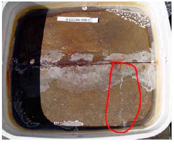

Figure 4.38. Photo. Traces of the upper three rebars and heavy corrosion products (specimen number 3-CCON-BB-1).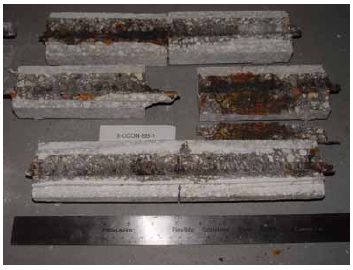

Figure 4.39. Photo. Trace of the upper rebars and heavy corrosion products on specimen number 1-STD1-BB-3.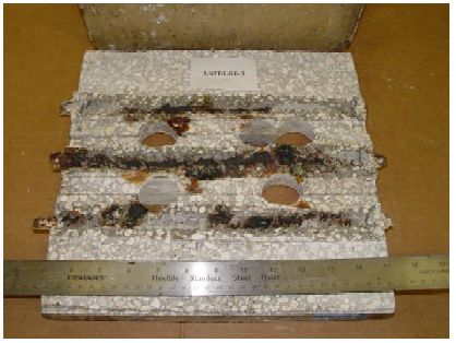

analyses, as evidenced by the two core holes that are seen in the figure. In both cases, considerable corrosion product buildup is apparent.

Slabs Reinforced With MMFX-II™ Bars

Figures 4.40 and 4.41 show potential and macro-cell current density results, respectively, for the STD1 MMFX-II™ bar slabs in comparison to the black bar slabs (figures 4.32 and 4.33). The initial potential decrease was similar for both bar types; however, this does not necessarily mean that time-to-corrosion was the same since different reinforcement types may have different potential criterion for activation. Current density, once corrosion initiated, was less for the MMFX-II™ reinforcement compared to black bar by about a factor of five (figure 4.41). This is consistent with potential of the MMFX-II™ bars having remained more positive that the black bars thereby resulting is reduced driving force for current flow. Likewise, figures 4.42 and 4.43 show similar plots for MMFX-II™ reinforced STD2 concrete specimens in comparison to the STD1 ones. These reveal more positive potentials and lower current densities for the lower w/c concrete (STD2) compared to the higher (STD1). Figures 4.44 through 4.55 show potential and macro-cell current density plots for specimens with, respectively, black bar cathode (BCAT), wire brushed bars (WB), top bar crevice or splice (CREV), cracked concrete (CCON), cracked concrete and crevice (CCRV), and cracked concrete and black bar cathode (CCNB). The effect of each of these factors on corrosion initiation and propagation is summarized in figure 4.56 which plots potential versus macro-cell current density for a single specimen in each category. As noted above for the comparable black bar specimens (figure 4.36), the data conform to a common trend, albeit with scatter, with data for the cracked concrete specimens (CCON and CCNB) generally falling in the relatively negative potential—high current density regime (similar to the comparable black bar specimens). Macro-cell current density data for the wire brushed bar specimens are generally less than for the other MMFX-II™ specimen types (see also figure 4.45).

Figure 4.40. Graph. Plot of potential versus exposure time for STD1 concrete specimens with MMFX-II™ reinforcement in comparison to black bar results.

Figure 4.41. Graph. Plot of macro-cell current density versus exposure time for STD1 concrete specimens with MMFX-II™ reinforcement in comparison to black bar results.

Figure 4.42. Graph. Plot of potential versus exposure time for STD1 and STD2 concrete specimens with MMFX-II™ reinforcement.

Figure 4.43. Graph. Plot of macro-cell current density versus exposure time for STD1 and STD2 concrete specimens with MMFX-II™ reinforcement.

Figure 4.44. Graph. Plot of potential versus exposure time for STD1 concrete specimens with black bar bottom mat and top mat MMFX-II™ reinforcement compared to ones with all MMFX-II™ bars.

Figure 4.45. Graph. Plot of macro-cell current density versus exposure time for STD1 concrete specimens with black bar bottom mat and top mat MMFX-II™ reinforcement compared to ones with all MMFX-II™ bars.

Figure 4.46. Graph. Plot of potential versus exposure time for STD1 concrete specimens with as-received and wire brushed (WB) MMFX-II™ reinforcement.

Figure 4.47. Graph. Plot of macro-cell current density versus exposure time for STD1 concrete specimens with as-received and wire brushed (WB) MMFX-II™ reinforcement.

Figure 4.48. Graph. Plot of potential versus exposure time for STD1 concrete specimens with top mat crevice bars (splice) and MMFX-II™ reinforcement compared to ones with normal bar placement.

Figure 4.49. Graph. Plot of macro-cell current density versus exposure time for STD1 concrete specimens with top mat crevice bars (splice) and MMFX-II™ reinforcement.

Figure 4.50. Graph. Plot of potential versus exposure time for STD1 concrete specimens with a simulated concrete crack and MMFX-II™ reinforcement compared to normal (uncracked) specimens.

Figure 4.51. Graph. Plot of macro-cell current density versus exposure time for STD1 concrete specimens with a simulated concrete crack and MMFX-II™ reinforcement compared to normal (uncracked) specimens.

Figure 4.52. Graph. Plot of potential versus exposure time for STD1 concrete specimens with a simulated concrete crack and MMFX-II™ reinforcement compared to ones with a simulated crack and top bar crevice (splice).

Figure 4.53. Graph. Plot of macro-cell current density versus exposure time for STD1 concrete specimens with a simulated concrete crack and MMFX-II™ reinforcement compared to ones with a simulated crack and top bar crevice (splice).

Figure 4.54. Graph. Plot of potential versus exposure time for STD1 concrete specimens with a simulated concrete crack and MMFX-II™ reinforcement compared to ones with a simulated crack and black bottom bars.

Figure 4.55. Graph. Plot of macro-cell current density versus exposure time for STD1 concrete specimens with a simulated concrete crack and MMFX-II™ reinforcement compared to ones with a simulated crack and black bar bottom mat.

Figure 4.56. Graph. Plot of potential versus macro-cell current density for MMFX-II™ reinforced specimens.

Figure 4.57 shows a photograph that was taken of the exposed surface of a MMFX-II™ specimen (specimen number 2-BCAT-MMFX-3) during the dry phase of the ponding cycle after 461 days. The surface is rust stained, and the concrete has cracked above one of the three bars. Likewise, Figures 4.58 through 4.65 show the appearance of the upper bar traces for one specimen each of the STD1, STD2, WB, CREV, CCON, BCAT, CCNB, and CCRV configurations. Because specimens were exposed at three different times but autopsied at the same time, the exposure time varied (566 to 707 days). Irrespective of this, a visual comparison of the standard STD1 and CCON black bar (figures 4.39 and 4.38, respectively) and companion MMFX-II™ specimens (figures 4.62 and 4.58, respectively) reveals considerably less corrosion for the latter, consistent with the corresponding current density data as discussed above. The visual extent of the corrosion products (figures 4.58 through 4.65) is generally consistent with magnitude of the long-term current density (higher current density, more corrosion). Bar traces on the autopsied MMFX-II™ BCAT specimen exhibited the greatest amount of corrosion product and had the highest current density at long-term. With the exception of the BCAT specimens, current density of the three specimen set of each type exhibited relatively little scatter.

Figure 4.57. Photo. Top surface of specimen 2-BCAT-MMFX-3 after 461 days of exposure.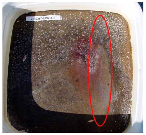

Figure 4.58. Photo. Trace of the upper rebars and corrosion products on specimen number 1-STD1-MMFX-2.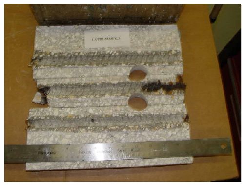

Figure 4.59. Photo. Trace of the upper rebars and corrosion products on specimen number 1-STD2-MMFX-2.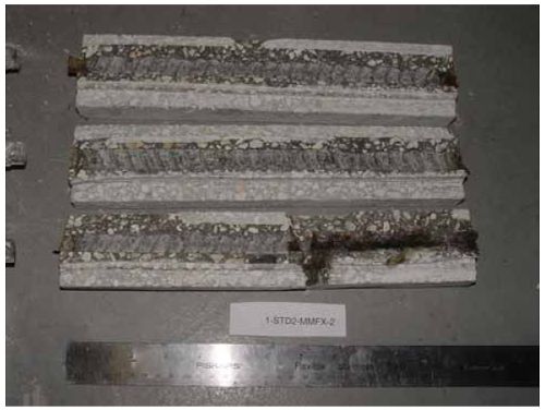

Figure 4.60. Photo. Trace of the upper rebars and corrosion products on specimen number 2-WB-MMFX-1.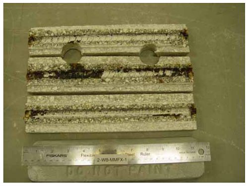

Figure 4.61. Photo. Trace of the upper rebars and corrosion products on specimen number 3-CREV-MMFX-1.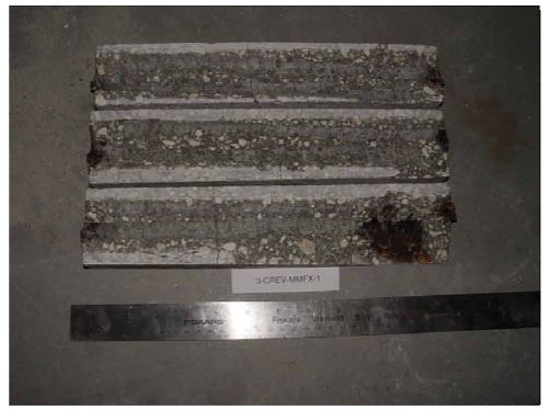

Figure 4.62. Photo. Trace of the upper rebars and corrosion products on specimen number 1-CCON-MMFX-1.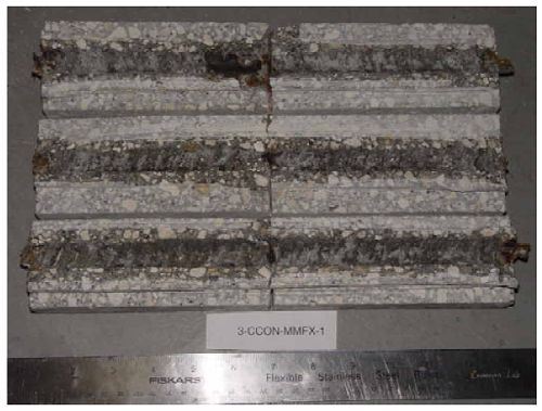

Figure 4.63. Photo. Trace of the upper rebars and corrosion products on specimen number 2-BCAT-MMFX-1.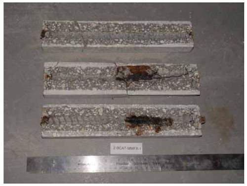

Figure 4.64. Photo. Trace of the upper rebars and corrosion products on specimen number 2-CCNB-MMFX-1.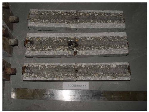

Figure 4.65. Photo. Trace of the upper rebars and corrosion products on specimen number 3-CCRV-MMFX-1.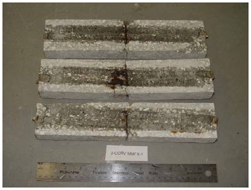

Slabs Reinforced With 3Cr12 Bars

Figures 4.66 through 4.79 present potential and macro-cell current density plots for specimens reinforced with 3Cr12.² For the standard STD1 specimens (figures 4.66 and 4.67), the corresponding black bar data are shown for comparison; and these reveal that, while the initial potential decay was approximately the same for the two reinforcements, macro-cell current density for the 3Cr12 reinforcement, once corrosion initiated, increased more gradually and to a steady-state value about three times lower than for the black bar specimens. Figure 4.80 shows a plot of potential versus macro-cell current density for specimens reinforced with 3Cr12 that includes representative data for each of the specimen types. As for the black bar and MMFX-II specimens, a common data band is apparent; however, in this case the band is more narrow and largely limited to a potential-current density regime rather than extending from upper left to lower right. The highest current densities occurred for specimens with concrete cracks (CCON and CCRV); however, this occurred also in the case for the black bar cathode (BCAT) specimens.

Photographs of the upper bar traces of autopsied specimens are shown in figures 4.81 through 4.87. These indicate that specimens STD1, STD2, CREV, and BCAT exhibited relatively heavy localized corrosion products on one bar compared to the WB, CCON, and CCRV specimens for which corrosion was relatively light. As for the MMFX-II™ specimens, the appearance of the corrosion products is in general agreement with the long-term current density data (higher current density greater corrosion products).

Figure 4.66. Graph. Plot of potential versus exposure time for STD1 concrete specimens with 3Cr12 reinforcement compared to that for black bar.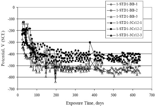

² Due to an error during specimen fabrication, six BCAT and no CCNB specimens with this reinforcement were prepared.

Figure 4.67. Graph. Plot of macro-cell current density versus exposure time for STD1 concrete specimens with 3Cr12 reinforcement compared to that for black bar.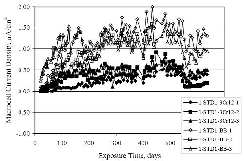

Figure 4.68. Graph. Plot of potential versus exposure time for STD1 and STD2 concrete specimens with 3Cr12 reinforcement.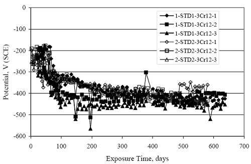

Figure 4.69. Graph. Plot of macro-cell current density versus exposure time for STD1 and STD2 concrete specimens with 3Cr12 reinforcement.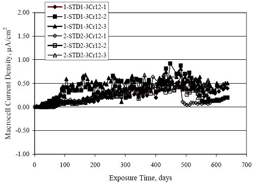

Figure 4.70. Graph. Plot of potential versus exposure time for STD1 concrete specimens with wire brushed compared to as-received 3Cr12 bars.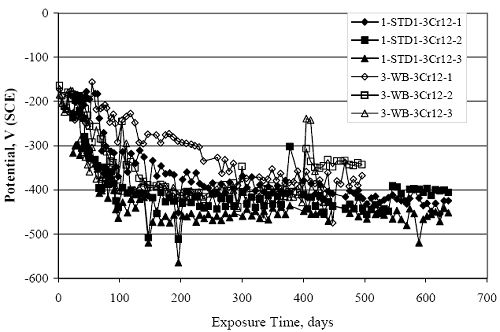

Figure 4.71. Graph. Plot of macro-cell current density versus exposure time for STD1 concrete specimens with wire brushed compared to as-received 3Cr12 bars.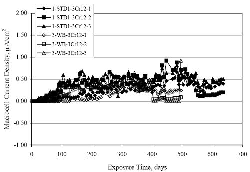

Figure 4.72. Graph. Plot of potential versus exposure time for STD1 concrete specimens with top mat bar crevice (splice) and 3Cr12 reinforcement compared to ones with normal bar placement.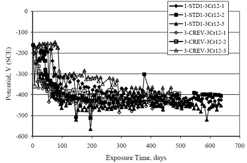

Figure 4.73. Graph. Plot of macro-cell current density versus exposure time for STD1 concrete specimens with top mat bar crevice (splice) and 3Cr12 reinforcement compared to ones with normal bar placement.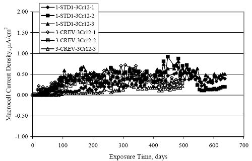

Figure 4.74. Graph. Plot of potential versus exposure time for STD1 concrete specimens with a simulated concrete crack and 3Cr12 reinforcement compared to uncracked ones.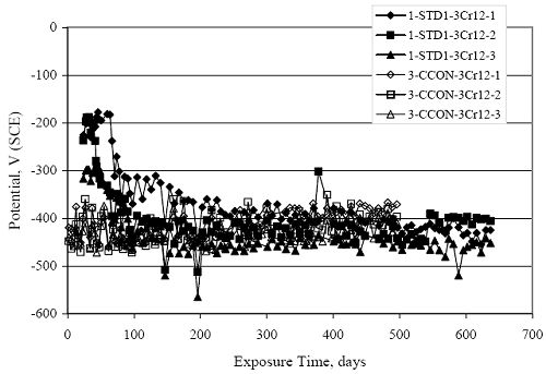

Figure 4.75. Graph. Plot of macro-cell current density versus exposure time for STD1 concrete specimens with a simulated concrete crack and 3Cr12 reinforcement compared to uncracked ones.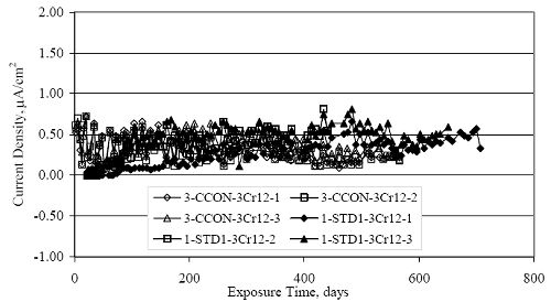

Figure 4.76. Graph. Plot of potential versus exposure time for STD1 concrete specimens with black bar bottom mat and top mat 3Cr12 reinforcement compared to ones with all 3Cr12 bars.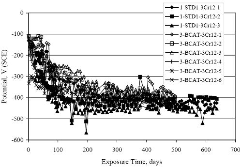

Figure 4.77. Graph. Plot of macro-cell current density versus exposure time for STD1 concrete specimens with black bar bottom mat and top mat 3Cr12 reinforcement compared to ones with all 3Cr12 bars.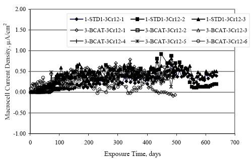

Figure 4.78. Graph. Plot of potential versus exposure time for STD1 concrete specimens with a simulated concrete crack and 3Cr12 reinforcement compared to cracked ones with a simulated crack and top bar crevice (splice).

Figure 4.79. Graph. Plot of macro-cell current density versus exposure time for STD1 concrete specimens with a simulated concrete crack and 3Cr12 reinforcement compared to cracked ones with a simulated crack and top bar crevice (splice).

Figure 4.80. Graph. Plot of potential versus macro-cell current density for 3Cr12 reinforced specimens.

Figure 4.81. Photo. Trace of the upper rebars and corrosion products on specimen number 1-STD1-3Cr12-1.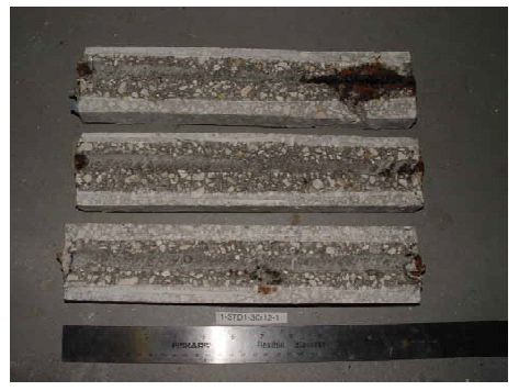

Figure 4.82. Photo. Trace of the upper rebars and corrosion products on specimen number 1-STD2-3Cr12-1.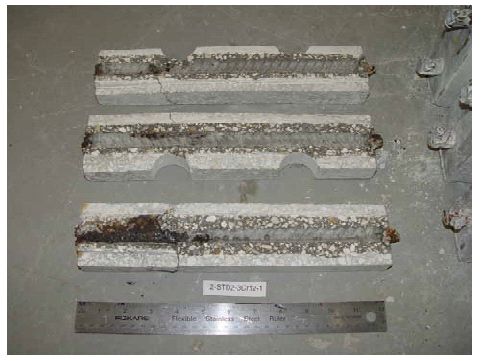

Figure 4.83. Photo. Trace of the upper rebars and corrosion products on specimen number 1-WB-3Cr12-1.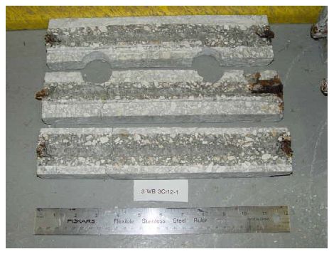

Figure 4.84. Photo. Trace of the upper rebars and corrosion products on specimen number 1-CREV-3Cr12-1.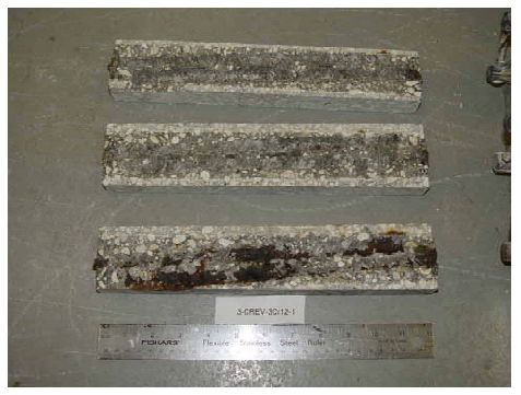

Figure 4.85. Photo. Trace of the upper rebars and corrosion products on specimen number 1-CCON-3Cr12-1.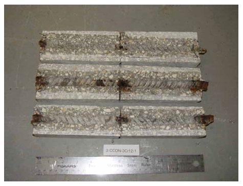

Figure 4.86. Photo. Trace of the upper rebars and corrosion products on specimen number 1-BCAT-3Cr12-1.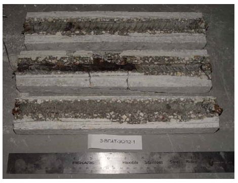

Figure 4.87. Photo. Trace of the upper rebars and corrosion products on specimen number 1-CCRV-3Cr12-1.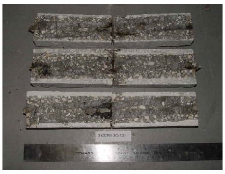

Slabs Reinforced With 2201 Bars

Figures 4.88 through 4.91 show potential and macro-cell current density plots for standard specimens reinforced with 2201. Here, the initial potential decay was more gradual than for the black bar specimens; and current density subsequent to initiation was less by a factor of 2 to 3. Figures 4.92 through 4.103 show plots for the other specimen variables. Figure 4.104 presents potential versus macro-cell current density data for specimens reinforced with 2201 that includes representative data for each of the specimen types. As for the other bar types, all data conform to a common trend but occupy different regimes therein. As such, the upper current densities of the trend band occurred for the crevice specimens (CCON and CCRV), whereas the wire brushed ones were at the lower bound. Some of the black cathode (BCAT) current densities occurred at values below the lower band bound. This apparently reflects the fact that potential remained relatively positive for one of the three specimens (see figure 4.98).

Figures 4.105 through 4.112 show photographs of the upper bar traces of autopsied specimens (one specimen from each group of three) for each of the specimen variables. These indicate that, more so than for the black bar, MMFX-II™, and 3Cr12, corrosion tended to initiate on the bars near the specimen side faces. Unlike the bar types evaluated above, corrosion products were more extensive on the STD2 than STD1 specimen (compare figures 4.105 and 4.106), which is inconsistent with the current density data (figure 4.91). The reason for this is unclear but may be related to the corrosion preferential attack at the bar ends. In addition to the STD2 specimen, products were extensive on at least one bar of the CREV, CCON, and BCAT specimens. Consequently, of the rebar types MMFX-II™, 3Cr12, and 2201, the autopsied CREV and BCAT specimens in each case exhibited heavy corrosion product accumulation on at least one of the three bars.

Figure 4.88. Graph. Plot of potential versus exposure time for STD1 concrete specimens with 2201 reinforcement compared to data for black bar.

Figure 4.89. Graph. Plot of macro-cell current density versus exposure time for STD1 concrete specimens with 2201 reinforcement compared to data for black bar.

Figure 4.90. Graph. Plot of potential versus exposure time for STD1 and STD2 concrete specimens with 2201 reinforcement.

Figure 4.91. Graph. Plot of macro-cell current density versus exposure time for STD1 and STD2 concrete specimens with 2201 reinforcement.

Figure 4.92. Graph. Plot of potential versus exposure time for STD1 concrete specimens with wire brushed (WB) 2201 bars compared to ones with as-received 2201 bars.

Figure 4.93. Graph. Plot of macro-cell current density versus exposure time for STD1 concrete specimens with wire brushed (WB) 2201 bars compared to ones with as-received 2201 bars.

Figure 4.94. Graph. Plot of potential versus exposure time for STD1 concrete specimens with top mat crevice bars (splice) and 2201 reinforcement compared to ones with normal bar placement.

Figure 4.95. Graph. Plot of macro-cell current density versus exposure time for STD1 concrete specimens with top mat crevice bars (splice) and 2201 reinforcement compared to ones with normal bar placement.

Figure 4.96. Graph. Plot of potential versus exposure time for STD1 concrete specimens with a simulated crack and 2201 reinforcement compared to uncracked ones.

Figure 4.97. Graph. Plot of potential versus exposure time for STD1 concrete specimens with a simulated crack and 2201 reinforcement compared to uncracked ones.

Figure 4.98. Graph. Plot of potential versus exposure time for STD1 concrete specimens with top mat 2201 bars and bottom mat black bar compared to ones with all 2201 bars.

Figure 4.99. Graph. Plot of macro-cell current density versus exposure time for STD1 concrete specimens with top mat 2201 bars and bottom mat black bar compared to ones with all 2201 bars.

Figure 4.100. Graph. Plot of potential versus exposure time for STD1 concrete specimens with a simulated concrete crack and 2201 reinforcement compared to ones with a simulated crack and black bottom bars.

Figure 4.101. Graph. Plot of macro-cell current density versus exposure time for STD1 concrete specimens with a simulated concrete crack and 2201 reinforcement compared to ones with a simulated crack and black bottom bars.

Figure 4.102. Graph. Plot of potential versus exposure time for STD1 concrete specimens with a simulated crack and crevice at top bars (splice) and 2201 reinforcement compared results for ones with cracked concrete and normal top bar placement.

Figure 4.103. Graph. Plot of macro-cell current density versus exposure time for STD1 concrete specimens with a simulated crack and crevice at top bars (splice) and 2201 reinforcement compared results for ones with cracked concrete and normal top bar placement.

Figure 4.104. Graph. Plot of potential versus macro-cell current density for 2201 reinforced specimens.

Figure 4.105. Photo. Trace of the upper rebars and corrosion products on specimen number 1-STD1-2201-3.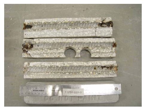

Figure 4.106. Photo. Trace of the upper rebars and corrosion products on specimen number 1-STD2-2201-2.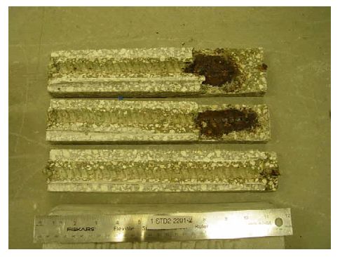

Figure 4.107. Photo. Trace of the upper rebars and corrosion products on specimen number 1-WB-2201-1.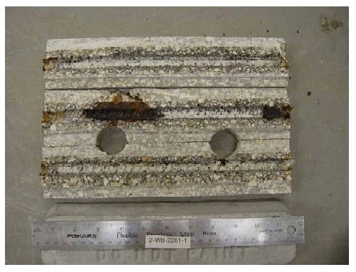

Figure 4.108. Photo. Trace of the upper rebars and corrosion products on specimen number 1-CREV-2201-1.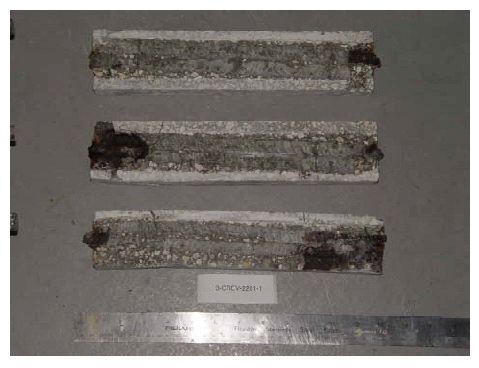

Figure 4.109. Photo. Trace of the upper rebars and corrosion products on specimen number 1-CCON-2201-1.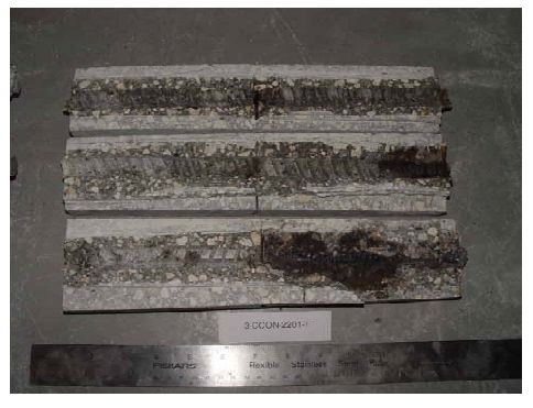

Figure 4.110. Photo. Trace of the upper rebars and corrosion products on specimen number 1-BCAT-2201-1.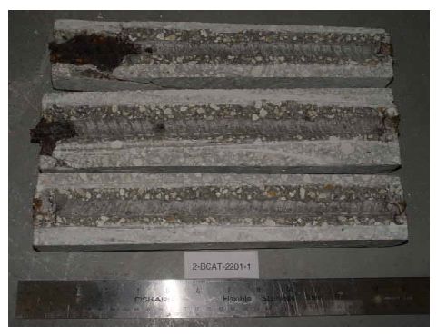

Figure 4.111. Photo. Trace of the upper rebars and corrosion products on specimen number 1-CCNB-2201-1.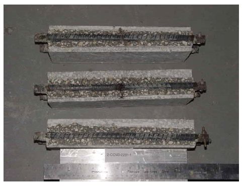

Figure 4.112. Photo. Trace of the upper rebars and corrosion products on specimen number 1-CCRV-2201-1.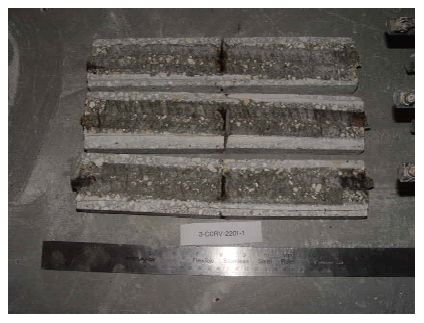

Figure 4.113 compares on a single plot the average macro-cell current density versus average potential data for each three specimen set (standard specimens only) of reinforcement types black bar, 3Cr12, MMFX-II™, and 2201 and illustrates that these conform to different trends. For black bar slabs, it was considered that active corrosion commenced once potential dropped to –280 mV_SCE, at which point the average macro-cell current density was about 0.26 μA/cm². If it is assumed that this same current density denotes onset of active corrosion for the other reinforcement types as well, then the corresponding potentials are –390, –350, and –195 mV_SCE for 3Cr12, MMFX-II™, and 2201, respectively. These potentials were achieved after 35 days (black bar), 64 to 140 days (3Cr12), 91 to 140 days (MMFX-II™), and 64 to 94 days (2201).

Slabs Reinforced With 316 Solid and Clad (Stelax) Stainless Bars

Figures 4.114 and 4.115 show plots of potential and macro-cell current density, respectively, for the standard solid and Stelax clad stainless steel specimens in comparison to that for the black bar ones. This reveals a general trend where potential of the stainless steel specimens tended to become more positive with exposure time with all specimens conforming to a common band. Macro-cell current density has remained nil throughout the exposures. Data for the BCAT, CREV, CCON, CCRV, and CCNB specimen types are not presented since potentials conformed to the same scatter band as for the standard specimens (figure 4.114), and macro-cell current density was nil in all cases.

Thus, for the standard specimen simulated deck slab configuration the reinforcement types rank from best to worst, as:

(4.2)

Figure 4.113. Graph. Plot of average potential versus average macro-cell current density at each measurement time for three specimens of the four indicated reinforcement types.

Figure 4.114. Graph. Plot of potential versus exposure time for STD1 and STD2 concrete specimens with 316.18, 316.17, and Stelax reinforcement compared to that for black bar in STD1 concrete.

Figure 4.115. Graph. Plot of macro-cell current density versus exposure time for STD1 and STD2 concrete specimens with 316.18 reinforcement compared to ones with black bar in STD1 concrete.

Chloride Concentration

At several times during the exposures, 76 mm diameter cores were taken at the mid-spacing between bars in two of the reinforced STD1 concrete slabs and from blank (nonreinforced) slabs that underwent the same ponding as the reinforced ones. The cores were then sliced, the slices ground to powder, and the powder analyzed for acid soluble [CL‾] using the FDOT stan dared method.¹⁹ Figure 4.116 shows the results as a plot of [CL‾] versus time and indicates that sorption probably contributed to transport of this species in the early stages of the exposures ([ CL‾] = 0.65 kg/m³ after a single ponding cycle (14 days)). Also apparent is that relatively high Cl‾ concentrations resulted during the time frame of the exposures ([ CL‾] ≈ 5 kg/m³ after about 100 days and 10 kg/m³ after 300 days).

Three Bar Columns

Square Three Bar Column Specimens

Figure 4.117 presents a time-to- corrosion (defined as potential achieving–280 mV_SCE) bar graph for all the S3BC specimens, where each bar in the plot represents the average of two or more specimens. In the case where corrosion has commenced for only one specimen, the total number of days of exposure is shown. The data indicate the following:

1. Black bar specimens had the shortest time-to-corrosion irrespective of mix design. This includes all six STD1 and STD2 specimens.
   

   Figure 4.116. Graph. Plot of chloride concentration at 2.54 cm below the exposed surface of STD1 concrete slabs versus exposure time.

   
   
   

   Figure 4.117. Graph. Time-to-corrosion results for square 3-bar column specimens.

   
2. All 3Cr12 specimens initiated corrosion, irrespective of mix design and specimen type.
3. Specimens reinforced with MMFX-II™ exhibited performance that was equivalent to 3Cr12 in the most aggressive conditions (control and bent bar groups) but outperformed 3Cr12 in the least aggressive cases (elevated bar and STD2 standard).
4. The 2201 reinforced specimens exhibited greater times-to-corrosion for all bars except 316.
5. Irrespective of concrete quality and specimen type, only 316 stainless steel has not initiated corrosion.
6. Bending the anode bar did not appear to have any effect on the time-to-corrosion of 316 and 2201 stainless steel reinforcements; but time-to-corrosion of 3Cr12 and MMFX-II™ was reduced by 47 and 41 percent, respectively.
7. Elevating the bar in the three bar columns resulted in a greater time-to-corrosion compared to the normal configuration (figures 3.19 and 3.20). However, all 3Cr12 and one 2201 specimen initiated corrosion in this configuration.
8. All reinforcement types performed better in the STD2 concrete than STD1 except for black bar, for which no difference was observed.
9. The following ranking resulted based on the time required for potential to shift to –280 mV_SCE or more negative (best to worst):
   

   (4.3)

   
   This is the same as for the simulated deck slab specimens, as indicated above, given that Stelax bars were not included in the three bar column test matrix.

Three Bar Tombstone Columns

Exposure of these specimens only commenced recently; and so there has been insufficient time to acquire meaningful results.

Macro-Cell Slab (MS) Specimens

Figure 4.118 shows a graph of typical potential and current trends with exposure time for macrocell slab specimens (MMFX-II™ in uncracked STD1 concrete in this case). The same criterion for defining corrosion initiation and time-to-corrosion was used as for the square three bar column specimens (potential ≤ –280 mV_SCE). However, in cases where a measurable macro-cell current increase occurred at a different time, corrosion initiation was defined as the time at which this current was detected. For this specimen group, specimen A initiated corrosion at 212 days, B at 69 days, and C after 231 days, for an average of 171 days.

Figure 4.119 shows time-to-corrosion data for STD1 MS specimens without a simulated crack. Based upon these results, the following conclusions were reached:

Figure 4.118. Graph. Example potential and current data for macro-cell slab specimens.

Figure 4.119. Graph. Time-to-corrosion results for the macro-cell slab specimens without a simulated crack.

1. Control STD1 specimens reinforced with black steel exhibited the shortest time-to-corrosion (black steel was not included in the other specimen types except as the cathode bar in the black steel cathode group). Ranking of the different reinforcements in the standard or control specimens was as listed below (best to worst):
   

   (4.4)

   
   

   This ordering is the same as for the simulated deck slab and three bar column specimens with the exception that 3Cr12 outperformed 2201 and MMFX-II™. Apparently, the fact that bars in the macro-cell slab specimens were wire brushed was responsible for this, although it cannot be ruled out that the difference in specimen design also may have been a factor. This performance reordering is surprising in the sense that wire brushing of the pickled 3Cr12 was of greater benefit than wire brushing of the as-rolled 2201. Time-to-corrosion of MMFX-II™ was essentially the same in each of the two surface conditions.

2. Reinforcements 3Cr12, MMFX-II™, and 2201 in the BCAT specimen configuration, exhibited greater times-to-corrosion than the corresponding controls. The reason for this improvement is unclear but will be investigated when the specimens are autopsied.
3. The 3Cr12, MMFX-II™, and 2201 reinforcements in the BNTB configuration (see table 3.7) all exhibited greater times-to-corrosion than did the respective controls (the improvement may not be significant in the case of 3Cr12), suggesting that the advantageous feature of either the BENT or BCAT configuration was retained in combination.
4. The best performance for each specimen type was exhibited by the 316 reinforcement. However, corrosion apparently initiated in one of the 316 BNTB specimens after approximately 260 days.

Figure 4.120 shows results for specimens with a simulated crack using the same format as in figure 4.119. This indicates that time-to-corrosion for black bar and 3Cr12 reinforced specimens was either relatively short (control specimens) or nil (BCAT and BENT configurations). The same was true for MMFX-II™ in the BNTB specimens. Otherwise, time-to-corrosion for the MMFX-II™ and 2201 specimens was comparable in general terms with that for the uncracked specimens. With the one exception noted above, none of the 316 reinforced specimens have initiated corrosion.

Field Columns

The field columns have been exposed for only 4 months. Currently, initial readings are all that are available, so there are no observations that can be made at this time.

Correlation of Concrete Specimen Data With Results From Accelerated Testing

Figure 4.121 shows a plot of time-to-corrosion for simulated deck slab and square three bar column specimens ens as a function of [CL‾_th] , as determined from the AST-2A experiments. This reveals a general trend where, with the exception of the 2201 simulated deck slab data, time-to

Figure 4.120. Graph. Time-to-corrosion results for the macro-cell slab specimens with a simulated crack.

Figure 4.121. Graph. Plot of time-to-corrosion of reinforced concrete specimens as a function of [ CL‾_th ] as determined from accelerated testing.

corrosion increased in proportion to [CL‾_th] . The error bands for the three bar column data correspond to one standard deviation, whereas for the simulated deck slabs these correspond to the data range. In comparing results for the two specimen types, the fact that corrosion of the simulated deck slab rebars may have initiated at or near the concrete interface because isolation was not provided here may have affected the results for these specimens. For most bar types in these specimens, concrete cracking, once this occurred, was along the line of the reinforcement; however, in the specific case of the 2201 specimens, cracking often occurred diagonally at the corners. This appeared to have resulted from corrosion of rebar near the concrete surface. Figure 4.122 is a photograph of an example case of this cracking. Subject to this limitation, the fact that time-to-corrosion increased in proportion to [CL‾_th] supports applicability of the AST-2A potentiostatic test method for projecting long-term reinforced concrete corrosion performance.

Figure 4.122. Photo. Example of corner cracking on a 2201 reinforced simulated deck slab specimen.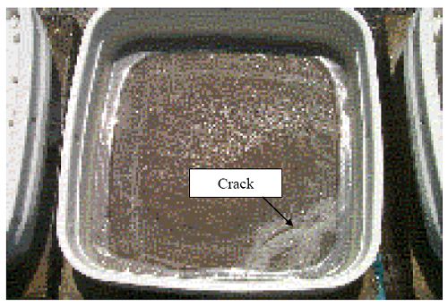

A calculation of time-to-corrosion, T_i, of STD1 concrete specimens was made based upon the [CL‾_th] projected for concrete from the AST-2A data (figure 4:31) using the one-dimensional solution for Fick’s second law,

(4.5)

where C_s. is [CL‾] at the exposed concrete surface, C₀ is the initial [ CL‾ ] in the concrete, and D_e is the effective diffusion coefficient. A determination of D_e was made from the average of two Clprofiles obtained after 136 days of exposure (see figure 4.116), which are shown in figure 4.123, using a least squares best fit algorithm to equation 4.4. This yielded a D_e of 3.20·10^-11 m²/s. Inputs to the Fick´s second law solution, in addition to this value for D_e, were cover 2.54·10^-2 m and C_s 18 kg/m³. Table 4.6 lists the calculated time-to-corrosion for black bar, 3Cr12, MMFXII™, and 2201. The projected times-to-corrosion are in general agreement with the measured values for concrete specimens (figure 4.121) with the exception of the 2201 reinforced simulated deck slab specimens, the reason being as discussed above.

Figure 4.123. Graph. Chloride profile from each of two cores taken from STD1 concrete slabs after 136 days of exposure.