U.S. Department of Transportation
Federal Highway Administration
1200 New Jersey Avenue, SE
Washington, DC 20590
202-366-4000
Federal Highway Administration Research and Technology
Coordinating, Developing, and Delivering Highway Transportation Innovations
 |
| This report is an archived publication and may contain dated technical, contact, and link information |
|
Publication Number:
FHWA-HRT-04-107
|
Previous | Table of Contents | Next
The engineering use of FRP piles on a widespread basis requires developing and evaluating reliable testing procedures and design methods that will help evaluate the load-settlement curve of these composite piles and their static bearing capacity. In particular, full-scale loading tests on FRP piles must be conducted to evaluate the behavior of these types of piles under vertical loads. The main objective of the study described in this chapter was to conduct a full-scale experiment (including dynamic and static load tests) on FRP piles, to address these engineering needs, and assess the feasibility of using FRP composite piles as vertical load-bearing piles. The full-scale experiment, described in this chapter, was conducted in a selected site of the Port Authority of New York and New Jersey at Port of Elizabeth, NJ. It included dynamic pile testing and analysis on 11 FRP driven piles and a reference steel pile, as well as SLTs on four FRP composite piles. Figure 39 shows the Port of Elizabeth demonstration site.
In this chapter, the results of SLTs are presented along with the instrumentation schemes that were specifically designed for strain measurements in the FRP piles. The experimental results are compared with current design codes and with the methods commonly used for evaluating the ultimate capacity, end bearing capacity, and shaft frictional resistance along the piles. This engineering analysis leads to preliminary recommendations for the design of FRP piles.
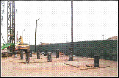
Figure 39. Photo. Port of Elizabeth demonstration site.
The FRP test piles were manufactured and instrumented to allow for the measurement of the load and settlements at the pile top, the displacements of the reaction dead load, and the axial strain at several levels in the pile to obtain the axial force variation with depth along the piles. The pile top settlements were measured by four linear variable differential transformers (LVDTs) (Model 10,000 hollow cylinder apparatus (HCA)), and the dead load displacements were measured by a LVDT (Model 5,000 HCA). Additional digital dial gauge indicators were also used to measure displacements. Vibrating wire and foil strain gauges were used to determine the axial force at several levels in the pile. The foil strain gauges were connected to a National Instruments data acquisition system, and the instrumentation of the pile head and the loading system was connected to a Geokon data acquisition system. The instrumentation and data acquisition systems (figures 40 through 42) allowed for online monitoring during the SLTs of: the pile top displacement versus the applied load; the applied load; and the stresses at different levels in the pile.
The manufacturers calibrated data acquisition with the LVDTs, the load cell, and the strain gauges before performing the field tests. All the strain gauges were installed in the FRP pile during the manufacturing process before the piles were delivered to the site. Pile manufacturing methods and instrumentation details are briefly described in the following paragraphs.
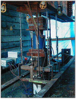
Figure 40. Photo. Equipment used in the in-load tests.
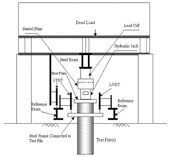
Figure 41. Illustration. Schematic of the equipment used in the in-load tests.
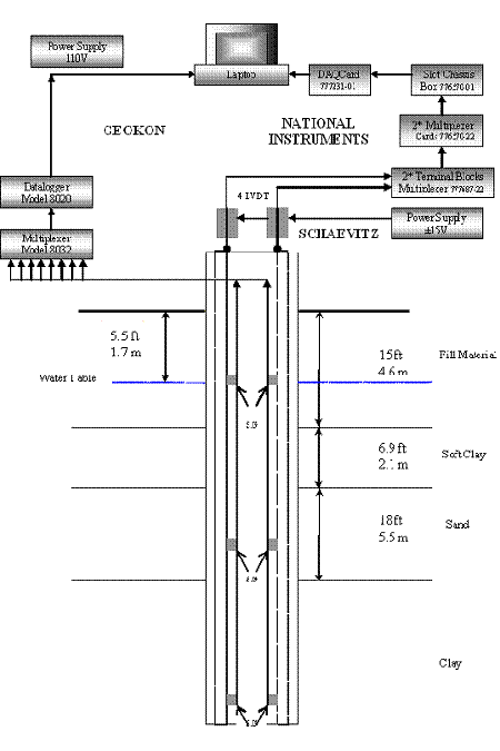
Figure 42. Illustration. Data acquisition system.
Lancaster Composite, Inc., piles are composed of a hollow FRP pipe that is filled before installation with an expanding concrete and is coated with a durable corrosion-resistant coating layer (figure 43). The hollow pipe is produced from unsaturated polyester or epoxy reinforced with reinforcement rovings (E-glass) and appropriate filler material to form a rigid structural support member. E-glass is incorporated as continuous rovings and is set in resin under pressure during the fabrication process. Table 2 shows the design material properties.
| Material Properties—FRP Shell for 16.5-inch outer diameter | |
|---|---|
| Young's modulus—axial (tensile) (psi) | 2.79 x 10⁶ |
| Tensile strength—axial direction (psi) | 50,400 |
| Young's modulus—axial (compression) (psi) | 1.9 x 10⁶ |
| Compressive strength—axial direction (psi) | 30,000 |
| Tensile strength—hoop direction (psi) | 35,000 |
| Elastic modulus—hoop direction (psi) | 4.5 x 10⁸ |
| Material Properties—Concrete Core for 16.5-inch outer diameter | |
| Concrete property (28 days)—fc prime (psi) | 6,000 |
| Expansion—confined permanent positive stress (psi) | 25 |
1 psi (lbf/in2) = 6.89 kPa
1 inch = 2.54 cm
The precast FRP composite pile (C40) is produced in two stages. The first stage consists of fabricating the hollow FRP tube, which is produced using the continuous filament winding method. The tube is given its final protective coating in the line during the winding process at the last station of the production line. During the second stage of the process, the tube is filled with an expanding cementious material at the plant.
Two vibrating wire strain gauges (model 4200VW) are installed 0.25 m (9.84 inches) from the bottom of the pile. The strain gauges were installed in the piles before the tube was filled with the cementious material. The installation procedure included casting strain gauges in the concrete (figure 43), inserting the strain gauge wires into the 1.9-cm- (0.75-inch-) diameter hollow fiberglass pipe, and locating the pipe in the center of the hollow FRP tubeusing steel spacers. At the end of the pile manufacturing process, concrete was cast into the FRP tube. To detect any zero drifts, strain readings were taken before strain gauge installation, after casting the concrete, before pile driving, and before performing the SLT.
Table 3 shows compressive laboratory test results performed on two samples that were taken from a concrete pile. The compressive strengths of the concrete after 28 days were 41,693 kPa (6,047 psi) and 43,609 kPa (6,325 psi), which are greater than the manufacturer's strength recommended values, by 0.8 percent and 5.4 percent, respectively.
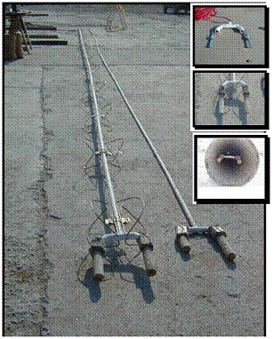
Figure 43. Photo. Strain gauges installation in pile of Lancaster Composite, Inc.
| Material Properties—Concrete Core for 16.5-inch O.D. | ||
|---|---|---|
| Test Number | Compression after 7 days, kPa (psi) | Compression after 28 days, kPa (psi) |
| 1 | 36,756 (5331) | 43,609 (6325) |
| 2 | 35,660 (5172) | 41,693 (6047) |
1 inch = 2.54 cm
PPI piles are composed of steel reinforcing bars that are welded to a spiral-reinforcing cage and encapsulated with recycled polyethylene plastic (figure 44). The manufacturing process uses a steel mold pipe and involves a combination of extrusion and injection molding, into which the plastic marine products are cast. Mold pipes for plastic pilings range in diameter from 20.3 cm (8 inches) to 121.9 cm (48 inches). The structural steel cage core is held at the center of the molded pile while the plastic is injected into the mold (figure 44). A centering apparatus is connected to the steel rebar cage so that it can be removed after the pile has been formed. Plastic is then fed into the extruder hopper through a mixing chamber, ensuring mixing with the carbon black material and the Celogen AZ130. The extruder temperature is set at 308 C (525 F). Plastic pressures range from 1.38 to 3.45 kPa (200 to 500 psi) throughout the mold while the plastic is being injected. After the extrusion process is complete, the mold is dropped into chilled water for a cooling period of several hours.
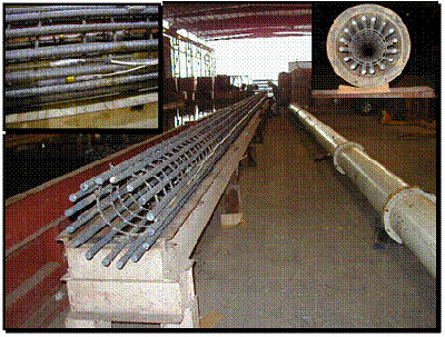
Figure 44. Photo. Vibrating and foil strain gauges attached to steel cage in PPI pile.
The strain gauges were installed in the piles at the company site before extruding the plastic material; therefore, the gauges and the cables had to resist high temperatures. Six vibrating wire strain gauges (model 4911-4HTX) were installed in the pile at 0.8 m (2.6 ft), 9.8 m (32.1 ft), and 18 m (59 ft) from the bottom. Two strain gauges were installed at each level. The strain gauges were attached to steel rebar and calibrated. Two additional foil strain gauges (model N2K-06-S076K-45C) were installed 0.8 m (2.6 ft) from the bottom of the pile. The foil strain gauges were attached to the steel rebar and sealed with epoxy glue to avoid moisture penetration. They then were assembled as a half-bridge and connected with the strain gauges located outside of the pile, creating a full Winston bridge. The installation process in the factory included welding the rebar with the strain gauges to the pile's steel reinforcement cage (figure 44). The strain gauges were connected to the data acquisition system to collect data before welding them to the steel cage, before extruding the hot plastic, and after cooling the pile down to detect any drifts of the zero reading. At the Port of Elizabeth, NJ, site, strain readings also were taken before pile driving and conducting the SLT.
SEAPILE composite marine piles contain fiberglass bars in recycled plastic material (figure 45). The manufacturing process of the SEAPILE composite marine piles consists of extruding the plastic material around the fiberglass bars using a blowing agent to foam to a density of 6.408 kN/m3 (40 lbf/ft3) at 217.5 C (380 F) and adding a black color for UV protection. The extrusion is followed by cooling the product and cutting to the desired length.
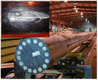
Figure 45. Photo. Vibrating and foil strain gauges attached to SEAPILE composite marine pile.
The strain gauges were installed at the factory after the pile was manufactured and the recycled plastic was cooled. Six vibrating wire strain gauges (model VK-4150)—two at each level—were installed in the pile 1 m (3.3 ft), 9.5 m (31.2 ft), and 18 m (59 ft) from the bottom. Two additional foil strain gauges (model EP-O8-250BF-350) were installed 1 m (3.3 ft) from the bottom of the pile. Each of these foil strain gauges was attached to plastic pieces by heating and sealing, using epoxy glue to avoid moisture penetration. The strain gauges were assembled to create a full Winston bridge. The installation procedure for the gauges included routing two grooves in the plastic material along the pile, providing an access to two rebar, and attaching the strain gauges and covering them by PC7 heavy duty epoxy paste. The wires in the groove were covered using hot, liquefied, recycled plastic.
The strain gauges were connected to the data acquisition system, and data were collected before connecting the gauges to the pile and after covering them with epoxy paste to detect any drift of the zero reading. Onsite strain readings also were taken before pile driving and before performing the SLT.
Figure 46 shows the schematic drawing of the Port Elizabeth site, and table 4 provides the testing program details, including pile structure, diameter, length, and the pile driving order. The test pile types included:
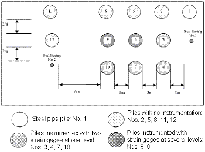
Figure 46. Illustration. Schematic drawing of Port Elizabeth site.
| Pile Type | Pile Structure | Driving Order Number | Ref. Number of Tested (SLT) Piles | Diameter cm (inch) | Length m (ft) | AE(1) kN (kips) |
|---|---|---|---|---|---|---|
| Steel Pile | Steel | 1 | — | 41.9 (16.5) | 20 (65.6) | — |
| Lancaster | Fiberglass cased concrete | 2,3,4 | 3 | 41.9 (16.5) | 18.8 (61.7) | 4.050 x 10⁶ (9.1 x 10⁵) |
| PPI | 16 steel bars 2.54 cm (1inch) in diameter in recycled plastic | 5,6,7 | 6 | 38.7 (15.25) | 19.8 (65.0) | 0.890 x 10⁶ (2 x 10⁵) |
| SEAPILE | 16 fiberglass bars 4.5 cm (1.75 inches) in diameter in recycled plastic | 8,9,10 | 9 | 42.5 (16.75) | 20 (65.6) | 0.745 x 10⁶ (1.67 x 10⁵) |
| American Ecoboard | Recycled plastic | 11,12 | 12 | 41.9 (16.5) | 6.1 (20) 11.8 (38.8) | — |
(1) A is area in square meters; E is Young's modulus in kilopascals, which is kilonewtons per square meter.
Port Elizabeth was constructed over a tidal marsh deposit consisting of soft organic silts, clays, and peats extending from mean high water to a depth of 3 to 9 m (10 to 30 ft). The site was reclaimed by placing fill over the marsh and surcharged to consolidate the compressible soils. The depth of the water table at the site is 1.7 m (5.5 ft) below the surface of the ground. Borings B-1 and B-2 indicated that the moisture content of the organic deposits ranged from 60 percent to 131 percent. The organic deposits are underlaid by silty fine sand. Below these materials are glacial lake deposits that generally range from sandy silt to clay and are sometimes varved. The glacial lake deposit at this site is overconsolidated. The consolidation test performed on a sample that was taken from this layer indicated a preconsolidation load of approximately 23 metric tons (t)/m2 (4.7 kips/ft2) and an overburden pressure of approximately 21.5 t/m2 (4.4 kips/ft2). The site is underlaid by shale rock. Two soil borings were performed: one near the steel pile, and the other near the American Ecoboard pile (figure 46). Soil laboratory tests show that the soil profiles can be roughly stratified into the layers in table 5.
| Depth, m (ft) | Soil Classification | Total Unit Weight, kN/m3 (lb/ft3) | Effective Cohesion, kN/m2 (psf) | Effective Friction Angle, Degrees |
|---|---|---|---|---|
| 0-4.6 (0-15) | SW-SC-Fill material | 20 (125) | 6 (125) | 35 |
| 4.6-6.7 (15-22) | OL-Organic clay with peat | 14.9 (93) | 1 (21) | 22 |
| 6.7-12.2 (22-40) | SM-Fine sand with silt | 20(125) | 6 (125) | 37 |
| 12.2-23.2 (40-76) | CL-Silt and clay | 19.4 (121) | 1 (21) | 23 |
| 23.2-25.9 (76-85) | Weathered shale | - | - | - |
| 25.9-29.7 (85-97.5) | Red shale | - | - | - |
Four SLTs were performed on the FRP piles 6 months after they were driven. This procedure allowed for dissipation of the excess pore water pressure that was generated in the clay layers during pile driving. The SLTs on the selected FRP piles were performed according to ASTM D-1143. Figures 47-50 illustrate the settlement-time records obtained during the SLTs. The load at each increment was maintained until the measured settlement was less than 0.001 mm (0.000039 inch). At each stage, an increment of 10 t (22 kips) were applied until the test ended or failure occurred.
Two loading cycles were performed in the SLTs on Lancaster Composite, Inc., and PPI piles. After loading to 100 t (220 kips) at the end of the first cycle, or to the maximum applied load, the piles were unloaded to zero load at 25-t (55-kip) increments.
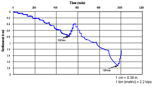
Figure 47. Graph. Lancaster pile—settlement-time relationship.
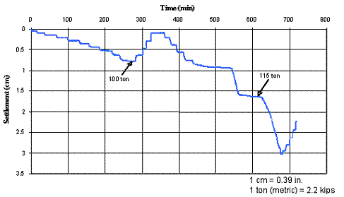
Figure 48. Graph. PPI pile—settlement-time relationship.
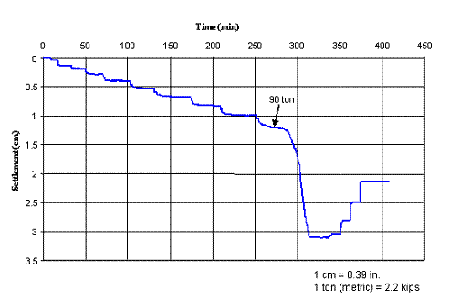
Figure 49. Graph. SEAPILE pile—settlement-time relationship.
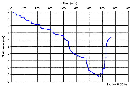
Figure 50. Graph. American Ecoboard pile—settlement-time relationship.
Vertical load-bearing capacity of piles depends mainly on site conditions, soil properties, method of pile installation, pile dimensions, and pile material properties. Full-scale SLTs (ASTM D-1143), analytical methods(26,27,28) based on pile and soil properties obtained from in situ or laboratory tests, and dynamic methods(8) based on pile driving dynamics are generally used to evaluate the static pile capacity. Testing procedures and design methods to determine the FRP composite pile capacities have not yet been established. For the purpose of this study, several analysis methods commonly used to design steel and concrete piles have been considered for evaluating the maximum load, end bearing, and shaft friction distribution along the FRP composite piles.
The offset limit method proposed by Davisson defines the limit load as the load corresponding to the settlement, S, resulting from the superposition of the settlement Sel due to the elastic compression of the pile (taken as a free standing column) and the residual plastic settlement Sres due to relative soil pile shear displacement.(26) The total settlement S can be calculated using the empirically derived Davisson's equation (figure 51).
![]()
Figure 51. Equation. Settlement, S.
Where:
Sel = PL/EA.
Sel = The settlement due to the elastic compression of a free standing pile column.
D = Pile diameter (m).
l = Pile length (m).
A = Pile cross section area (m2).
e = Pile Young's modulus (kPa).
P = Load (kN).
The limit load calculated according to this method is not necessarily the ultimate load. The offset limit load is reached at a certain toe movement, taking into account the stiffness, length, and diameter of the pile. The assumption that the elastic compression of the pile corresponds to that of a free-standing pile column ignores the load transfer along the pile and can, therefore, lead to overestimating the pile head settlement, particularly for a friction pile. Because of the load transfer along the pile, the settlement corresponding to the elastic compression generally does not exceed 50 percent of the elastic settlement for a free-standing column.
Pile data used to calculate the ultimate capacities according to the Davisson offset limit load method for FRP piles are summarized in table 6. The elastic properties of pile materials were determined by laboratory compression tests on full-section composite samples.
Figures 52-55 show the load versus pile head settlement curves measured during the SLTs. As illustrated in these figures, Davisson's limit method is used to establish the limit loads under the following assumptions:
Comparing the results obtained with the Davisson's procedure for these three assumptions and load-settlement curves obtained from the static loading tests, it can be concluded that for the highly compressible FRP piles, the assumption that the pile elastic compression is equivalent to that of a free-standing column leads to greatly overestimating the pile head settlement. The assumption that an equivalent elastic modulus of the composite pile can be derived from the slope of the load-settlement curve that is defined from an unloading-reloading cycle leads to settlement estimates that appear to be quite consistent with the experimental results. Further, these settlements are also quite close to the settlements, due to the elastic compression calculated for the friction piles, assuming a constant load transfer rate along the pile (i.e., about 50 percent of the elastic compression of a free-standing pile column). For the American Ecoboard pile that was driven to the sand layer, the load-settlement curve did not reach any plunging failure. For this pile, the Davisson's procedure that considers the equivalent elastic modulus derived from the unloading-reloading load-settlement curve yields estimates of the limit load (about 50 t) and pile head settlement (about 6 cm (2.4 inches)), which appear to be consistent with the experimental results.
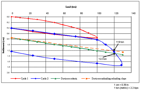
Figure 52. Graph. Lancaster Composite pile—Davisson criteria and measured load-settlement curve.
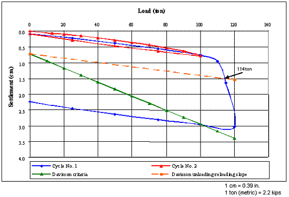
Figure 53. Graph. PPI pile—Davisson criteria and measured load-settlement curve.
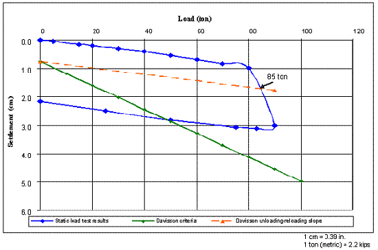
Figure 54. Graph. SEAPILE pile—Davisson criteria and measured load-settlement curve.
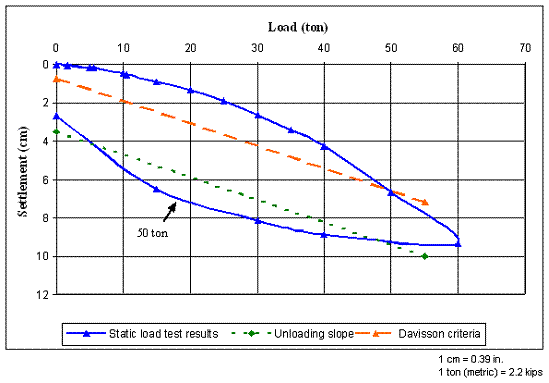
Figure 55. Graph. American Ecoboard pile—Davisson criteria and measured load-settlement curve.
The DeBeer ultimate capacity is determined by plotting the load-settlement curve on a log-log scale diagram.(27) As illustrated in figure 56, on the bilinear plot of the load versus settlement, the point of intersection (i.e., change in slope) corresponds to a change in the response of the pile to the applied load before and after the ultimate load has been reached. The load corresponding to this intersection point is defined by DeBeer as the yield load. Figure 56 shows the DeBeer criteria as plotted for the FRP piles. The DeBeer yield loads are 110 t (242 kips) for the Lancaster Composite, Inc., and PPI piles and 80 t (176 kips) for the SEAPILE pile. The yield load for the American Ecoboard pile could not be defined. This pile did not experience a plunging failure during the SLT.
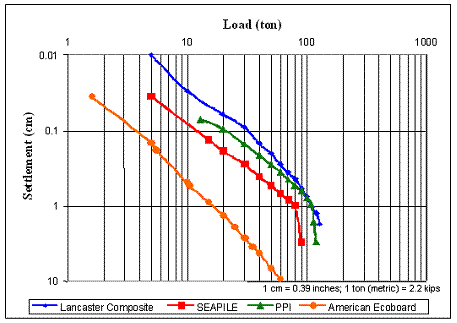
Figure 56. Graph. DeBeer criterion plotted for FRP piles.
Chin(28) proposed an application of the Kondner(29) method to determine the failure load. As illustrated in figure 57, the pile top settlement is plotted versus the settlement divided by the applied load, yielding an approximately straight line on a linear scale diagram. The inverse of the slope of this line is defined as the Chin-Kondner failure load. The application of the Chin-Kondner method for the engineering analysis of the SLTs conducted on the FRP piles, illustrated in figure 57, yields the ultimate loads of 161 t (354 kips), 96 t (211 kips), and 125 t (275 kips) for the Lancaster Composite, Inc., SEAPILE, and PPI piles, respectively.
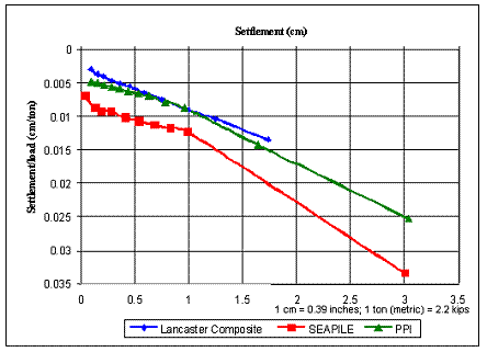
Figure 57. Chin-Kondner method plotted for FRP piles.
Applying the Chin-Kondner method for the American Ecoboard pile, illustrated in figure 58, yields a failure load of approximately 102 t (224 kips).
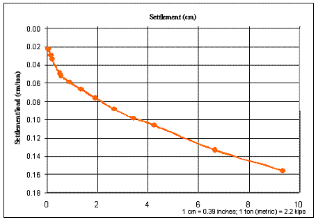
Figure 58. Chin-Kondner method plotted for American Ecoboard pile.
The application of the Chin-Kondner method yields a failure load that is defined as the asymptotic ultimate load of the load-settlement curve. It therefore yields an upper limit for the failure load leading in practice to overestimating the ultimate load.
However, if a distinct plunging ultimate load is not obtained in the test, the pile capacity or ultimate load is determined by considering a specific pile head movement, usually 2 to 10 percent of the diameter of the pile, or a given displacement, often 3.81 cm (1.5 inches). As indicated by Felenius, such definitions do not take into account the elastic shortening of the pile, which can be substantial for composite long piles such as FRP piles.(30)
| Pile Manufacturer | Static Load Test Results | Davisson Offset Limit Load | DeBeer Yield Load | Chin-Kondner | Davisson Criteria Un/reloading Slope | |||||
|---|---|---|---|---|---|---|---|---|---|---|
| Load t | Settlement cm | Load t | Settlement cm | Load t | Settlement cm | Load t | Settlement cm | Load t | Settlement cm | |
| Lancaster Composite(1) | 128 | 1.73 | 122 | 1.31 | 110 | 0.96 | 161 | - | 119 | 1.3 |
| PPI | 115 | 1.64 | 121 | 3.40 | 110 | 0.96 | 125 | - | 114 | 1.5 |
| SEAPILE | 90 | 1.16 | 92 | 4.60 | 80 | 0.98 | 96 | - | 85 | 1.8 |
| American Ecoboard(1) | 60 | 9.34 | - | - | - | - | 102 | - | 50 | 6.0 |
(1) The pile did not experience plunging failure during the static load test. 1 cm = 0.39 inch; 1 t = 2.2 kips
Table 6 summarizes the maximum loads applied during the SLTs and the ultimate loads calculated using the Davisson offset limit load, DeBeer yield load, and the Chin-Kondner methods. Distinct plunging failure occurred during the SLTs on PPI and SEAPILE piles as the applied loads reached 115 and 90 t (253 and 198 kips) and the measured pile top settlements were 1.64 cm (0.65 inch) and 1.16 cm (0.46 inch), respectively. The Lancaster Composite, Inc., pile did not experience a distinct plunging failure, and as the maximum load applied on the pile reached 128 t (282 kips), the measured settlement was 1.73 cm (0.68 inch). The maximum load applied on the American Ecoboard pile was 60 t (132 kips). At this load, the pile top settlement was 9.34 cm (3.7 inches), and no distinct plunging was observed. The pile top settlements of this pile, which contains only recycled plastic with no reinforcement bars, were significantly greater than the settlements measured during the tests on the other FRP piles (figures 52 through 57).
The Davisson's offset limit is intended primarily to analyze test results from driven piles tested according to quick testing methods (ASTM D-1143) and, as indicated by Fellenius, it has gained widespread use with the increasing popularity of wave equation analysis of driven piles and dynamic testing.(31) This method allows the engineer, when proof testing a pile for a certain allowable load, to determine in advance the maximum allowable movement for this load considering the length and dimensions of the pile.(32) The application of the Davisson's offset limit load method illustrates that for the compressible FRP piles, the effect of load transfer along the piles must be considered in estimating the maximum allowable pile movement. The equivalent elastic modulus of the composite pile derived from the measured pile response to the unloading-reloading cycle leads to settlement estimates that are quite consistent with the experimental results.
The DeBeer yield load method was proposed mainly for slow tests (ASTM D-1143).(33) In general, the loads calculated by this method are considered to be conservative. The calculated loads for the Lancaster Composite, Inc., and PPI piles (110 t (242 kips)), and for the SEAPILE pile, (80 t (176 kips)), are smaller than the maximum load applied on these piles by 14 percent, 4 percent, and 11 percent, respectively. For these calculated loads, the calculated settlements for the Lancaster Composite, Inc., PPI, and SEAPILE piles are smaller than the measured settlements by 44.5 percent, 41.5 percent, and 15.5 percent, respectively.
The Chin-Kondner method is applicable for both quick and slow tests, provided constant time increments are used. As indicated by Fellenius,(30) during a static loading test, the Chin-Kondner method can be used to identify local low resistant zones in the pile, which can be of particular interest for the composite FRP piles.
As an approximate rule, the Chin-Kondner failure load is about 20 to 40 percent greater than the Davisson limit.(30) As shown in table 6, all the loads calculated by the Chin-Kondner method were greater than the maximum load applied on the piles in the field test. The calculated loads for the Lancaster Composite, Inc., PPI, SEAPILE, and American Ecoboard piles, 161, 125, 96, and 102 t (354, 275, 211, and 224 kips), are greater than the Davisson offset limit load by 32 percent, 3 percent, 4 percent, and 30 percent, respectively.
In general, the ultimate loads calculated for FRP piles using the Chin-Kondner method are greater than the maximum loads applied in the field test. The DeBeer yield load method yields conservative loads in comparison to the maximum loads obtained at the SLTs. The Davisson offset limit load method, using the equivalent elastic modulus obtained from the pile response to an unloading-reloading cycle, yields ultimate loads that are within the range of loads obtained with the above-mentioned methods and allowable settlements that are close to the settlements reached with maximum loads applied in the field tests.
Axial load-bearing capacity, end bearing, and shaft friction along the pile can be evaluated using analytical methods based on pile and soil properties obtained from in situ and/or laboratory tests. For the purpose of the SLT engineering analysis, the experimental results were compared with several commonly used methods, including the "alpha" total stress analysis and the "beta" effective stress analysis. A state-of-the-art review on foundations and retaining structures presented by Poulos, et al., (briefly summarized below) relates to axial capacity of piles.(34) An estimate of a pile's ultimate axial load-bearing capacity can be obtained by the superposition of the ultimate shaft capacity, Psu, and the ultimate end bearing capacity, Pbu. The weight, Wp, of the pile is subtracted for the compressive ultimate load capacity. For compression, then, the ultimate load capacity, Puc, is given by the equation in figure 5.
![]()
Figure 59. Equation. Ultimate load capacity Puc.
Where:
fs = Ultimate shaft friction resistance in compression (over the entire embedded length of the pile shaft).
C = Pile perimeter.
dz = Length of the pile in a specific soil layer or sublayer.
fb = Ultimate base pressure in compression.
Ab = Cross-sectional area of the pile base.
Commonly, the alpha method is used to estimate the ultimate shaft friction in compression,fs, for piles in clay soils. The equation in figure 60 relates the undrained shear strength su to fs.
![]()
Figure 60. Equation. Ultimate shaft friction in compression fs.
Where:
a = Adhesion factor.
The ultimate end bearing resistance fb is given by the equation in figure 61.
![]()
Figure 61. Equation. Ultimate end bearing resistance fb.
Where:
Nc = Bearing capacity factor.
Several common approaches used for estimating the adhesion factor a for driven piles are summarized in table 7. Other recommendations for estimating a, for example, in Europe, are given by De Cock.(35) For pile length exceeding about three to four times the diameter, the bearing capacity factor Nc is commonly taken as 9.
A key difficulty in applying the total stress analysis is estimating the undrained shear strength su. It is now common to estimate su from in situ tests such as field vane tests or cone penetration tests, rather than estimating it from laboratory unconfined compression test data. Values for su can vary considerably, depending on the test type and the method of interpretation. Therefore, it is recommended that local correlations be developed for a in relation to a defined method of measuring su.(34)
| Pile Type | Remarks | Reference |
|---|---|---|
| Driven | α = 1.0 (su ≤ 25 kPa)
α = 0.5 (su ≥ 70 kPa)
Interpolate linearly between |
API(6) |
| Driven | α = 1.0 (su ≤ 25 kPa)
α = 0.5 (su ≥ 70 kPa)
Linear variation between
length factor applies for L/d ≥ 50 |
Semple and Rigden(36) |
| Driven | α = (su/σ'v) 0.5 (su/σ'v) -0.5 for (su/σv') ≤ 1
α = (su/σ'v) 0.5 (su/σ'v) -0.25
for (su/σv') ≥ 1 |
Fleming, et al.(37) |
For any soil type, the beta effective stress analysis may be used for predicting pile capacity. The relationship between fs and the in situ effective stresses may be expressed by the equation in figure 62.
![]()
Figure 62. Equation. Relationship between fs and in situ stresses.
Where:
Ks = Lateral stress coefficient.
δ = Pile-soil friction angle.
σ'v = Effective vertical stress at the level of point under consideration.
A number of researchers have developed methods of estimating the lateral stress coefficient Ks. Table 8 summarizes several approaches, including the commonly used approaches of Burland(38) and Meyerhof.(4)
| Pile Type | Soil Type | Details | Reference |
|---|---|---|---|
| Driven and Bored | Sand | Ks = A + BN
where N = SPT (standard penetration test) value
A = 0.9 (displacement piles)
Or 0.5 (nondisplacement piles)
B = 0.02 for all pile types |
Go and Olsen(39) |
| Driven and Bored | Sand | Ks = Ko (Ks/Ko)
where Ko= at-rest pressure coefficient
(Ks/Ko) depends on installation method; range is 0.5 for jetted piles to up to 2 for driven piles |
Stas and Kulhawy(40) |
| Driven | Clay | Ks= (1 - sin φ') (OCR) 0.5
where φ' = effective angle of friction
OCR = overconsolidation ratio;
Also, δ = φ |
Burland(38) Meyerhof(4) |
SPT test result data imply the empirical correlations expressed in figures 63 and 64.
![]()
Figure 63. Equation. Empirical correlations for shaft friction.
Where:
AN and BN = Empirical coefficients.
N = SPT blow count number at the point under consideration.
![]()
Figure 64. Equation. Empirical correlation for end bearing resistance.
Where:
CN = Empirical factor.
Nb = Average SPT blow count within the effective depth of influence below the pile base (typically one to three pile base diameters).
Meyerhof recommended using AN = 0, BN = 2 for displacement piles and 1 for small displacement piles, and CN = 0.3 for driven piles in sand.(41) Limiting values of fs of about 100 kPa (14.5 psi) were recommended for displacement piles and 50 kPa (7.25 psi) for small displacement piles. Poulos summarized other correlations, which include several soil types for both bored and driven piles.(42) Decourt's recommendations included correlations between fs and SPT, which take into account both the soil type and the methods of installation.(43) For displacement piles, AN = 10 and BN = 2.8, and for nondisplacement piles, AN = 5-6 and BN = 1.4-1.7. Table 9 shows the values of CN for estimating the end bearings. Rollins et al. discussed the correlations for piles in gravel.(44) The correlations with SPT must be treated with caution, as they are inevitably approximate, and are not universally applicable.(34)
| Soil Type | Displacement Piles | Nondisplacement Piles |
|---|---|---|
| Sand | 0.325 | 0.165 |
| Sandy silt | 0.205 | 0.115 |
| Clayey silt | 0.165 | 0.100 |
| Clay | 0.100 | 0.080 |
SLT results were compared with several design codes(5-7) and methods commonly used(4) for evaluating the end bearing and shaft friction along the pile. Figures 65, 66, and 67 show the loads versus depth measured in the SLTs for PPI, SEAPILE, and Lancaster Composite, Inc., piles, respectively.
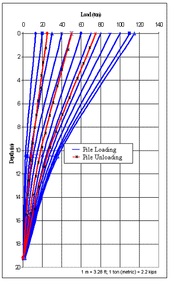
Figure 65. Graph. PPI pile, measured loads versus depth.
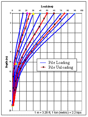
Figure 66. Graph. SEAPILE pile, measured loads versus depth.
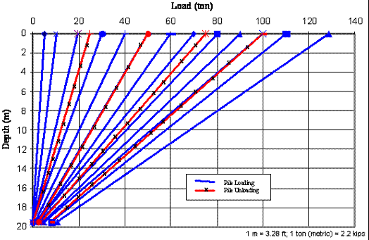
Figure 67. Graph. Lancaster Composite, Inc., pile, measured loads versus depth.
As illustrated in these figures, the axial force distribution measured along the piles indicates that the FRP piles at the Port Elizabeth site were frictional piles, with maximum end bearing capacities, which were equal to 1.6 percent, 1.0 percent, and 8.4 percent of the total applied load for the PPI, SEAPILE, and the Lancaster Composite, Inc. piles, respectively.
| Static Load Test Results | Go and Olsen(39) | Stas and Kulhawy(40) | FHWA (5) | API (6) | Meyerhof (4) | AASHTO (7) | |||
|---|---|---|---|---|---|---|---|---|---|
| PPI | SEAPILE | Lancaster Composite | |||||||
| End bearing capacity, t | 1.9 | 0.9 | 10.8 | - | - | 73.5 | 6.6 | 75.4 | - |
| Total shaft friction, t | 113.1 | 89.1 | 117.7 | 11.3 | 7.33 | 49.7 | 81 | 4.3 | 16.4 |
| Shaft friction depth 0 to 10 m, t/m2 | 6.0 | 5.6 | - | 2.9 | 2.0 | 2.4 | 4.0 | 4.5 | 7.3 |
| Shaft friction depth 10 to 20, t/m2 | 3.15 | 1.65 | - | 9.1 | 5.8 | 2.6 | 8.8 | 6.8 | 1.2 |
| Shaft friction depth 0 to 20, t/m2 | 4.5 | 3.5 | 4.7 | 4.5 | 2.6 | 4 | 6.4 | 5.6 | 4.2 |
| Total capacity, t | 115 | 90 | 128.5 | - | - | 123.2 | 87.6 | 79.7 | - |
| End bearing capacity Total load, % | 1.6 | 1.0 | 8.4 | - | - | 59.7 | 7.5 | 94.6 | - |
1 t = 2.2 kips; 1 m = 3.28 ft
Table 10 summarizes the comparison of the average measured shaft friction along the FRP piles and the shaft friction values calculated from several design codes and methods of analysis commonly used. The engineering analysis of the shaft friction distribution takes into consideration two soil layers corresponding to the upper soil layers from 0 to 10 m (32.8 ft), which consists of fill material, a soft clay layer, and a sandy layer, and the lower soil layer from 10 to 20 m (32.8 to 65.6 ft), which consists of a 3-m (9.8-ft) sand layer overlaying a 7-m (23-ft) clay and silt layer. Average values of the shaft friction also are obtained, taking into account the axial force measured at the top and the bottom of the soil. For the PPI and SEAPILE piles, the average shaft friction values obtained at the upper 10-m (32.8-ft) layer were greater than the shaft friction values measured at the lower clay layer. The Burland and Meyerhof methods and the AASHTO code appear to yield the best correlation for shaft friction values in the upper layer. The FHWA code appears to yield the best correlation for the shaft friction values obtained in the lower clay and silt layer.

