Bottomless Culvert Scour Study: Phase I Laboratory Report
4. RESULTS
SCOUR RESULTS
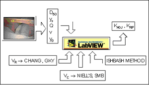
Extensive analysis was performed using various combinations of equations for resultant velocity and critical velocity. Figure 22 shows how the experimental data was processed and the different evaluation methods used to derive the adjustment coefficients. This section presents the results using the Maryland DOT (Chang) and GKY methods for representative velocity and critical velocity, and the combination that yielded the best results.
Figure 22. Post-processing: data analysis flow chart.
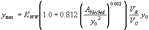
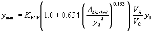
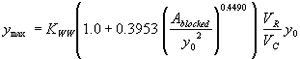
The regression analysis was performed for two sets of data: data for the vertical face and data for the wingwall entrances. Separate equations were derived for the two data sets; however, we determined that the two equations could be combined into one general equation by incorporating an entrance coefficient (KWW) to account for the streamlining effects of the wingwalls. Equation 34 is the general expression for the maximum depth to be expected at the upstream corners of a bottomless culvert with no upstream sediment being transported into the scour hole.
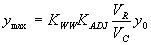 (34) where:
| KWW | = wingwall entrance coefficient |
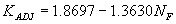
| KADJ | = empirical adjustment factor to account for turbulence and vorticity at the upstream corner of the culvert derived from regression analysis |
We used R2 and MSE to indicate which combinations of representative velocity, critical velocity, and independent regression variables worked best for this data.
Maryland DOT (Chang) Method for Representative Velocity and Critical Velocity
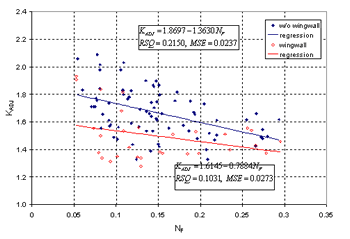
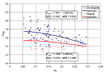
Four different independent regression variables were tested for the Maryland DOT method. One of these, the Froude number (NF) (originally the Chang method), was compared to KADJ using three different regression methods: linear, second order, and quadratic. The linear regression gave R2 values of 0.22 for the vertical face data and 0.10 for the wingwall data (figures 23 and 24, respectively).
Figure 23. Maryland DOT's (Chang's) resultant velocity with Chang's approximation equation and local scour ratio as a function of the Froude number, using a linear regression.
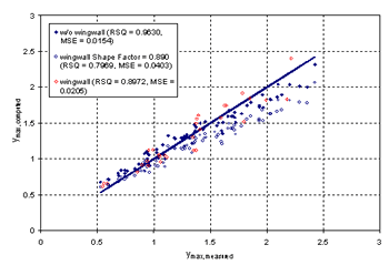
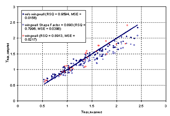
Figure 24. Measured and computed data with and without wingwalls, based on figure 23 regression.
Incorporating the adjustment function from figure 23 leads to the general equation:
 (35) where:
| KWW | = 1.0 for vertical face entrances
= 0.89 for wingwall entrances |
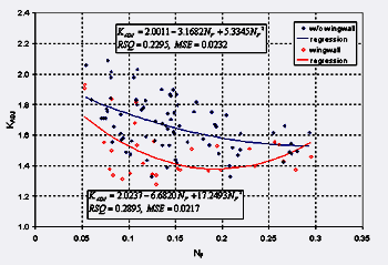
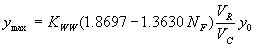
The Froude number (NF) with a second order regression gave R2 values of 0.35 for the vertical face data and 0.28 for the wingwall data (figures 25 and 26, respectively).
Figure 25. Maryland DOT's (Chang's) resultant velocity with Chang's approximation equation for critical velocity and local scour ratio as a function of the Froude number, using a second order regression.
Figure 26. Measured and computed data with and without wingwalls, based on figure 25 regression.
Incorporating the adjustment function from figure 25 leads to the general equation:
 (36) where:
| KWW | = 1.0 for vertical face entrances
= 0.89 for wingwall entrances |
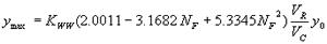
The Froude number (NF) with a quadratic regression gave R2 values of 0.15 for the vertical face data and 0.06 for the wingwall data (figures 27 and 28, respectively).
Figure 27. Maryland DOT's (Chang's) resultant velocity with Chang's approximation for critical velocity and local scour ratio as a function of the Froude number, using a linear regression.
Figure 28. Measured and computed data with and without wingwalls, based on figure 27 regression.
Incorporating the adjustment function from figure 27 leads to the general equation:
 (37) where:
| KWW | = 1.0 for vertical face entrances
= 0.89 for wingwall entrances |
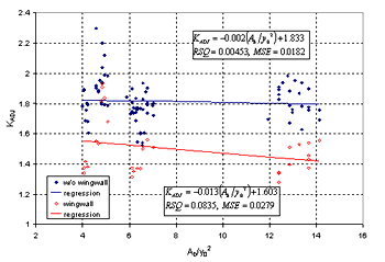
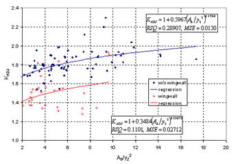
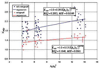
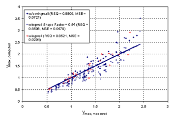
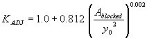
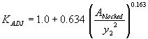
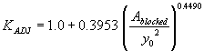
Using the approach flow area that is blocked by the embankments on one side of the channel over the squared flow depth as the independent regression variable yielded R2 values of 0.004 for the vertical face data and 0.08 for the wingwall data (figures 29 and 30, respectively).
Figure 29. Maryland DOT's (Chang's) resultant velocity with Chang's approximation for critical velocity and local scour ratio as a function of the blocked area over the squared flow depth.
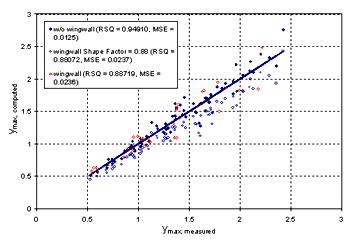
Figure 30. Measured and computed data with and without wingwalls, based on figure 29 regression.
Incorporating the adjustment function from figure 29 leads to the general equation:
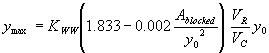 (38) where:
| KWW | = 1.0 for vertical face entrances
= 0.88 for wingwall entrances |
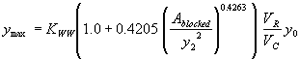
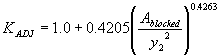
The third independent regression variable tested was the approach flow area that is blocked by the embankments on one side of the channel over the squared computed equilibrium depth, resulting in R2 values of 0.29 for the vertical face data and 0.11 for the wingwall data (figures 31 and 32, respectively).
Figure 31. Maryland DOT's (Chang's) resultant velocity with Chang's approximation for critical velocity and local scour ratio as a function of the blocked area over the squared computed equilibrium depth.
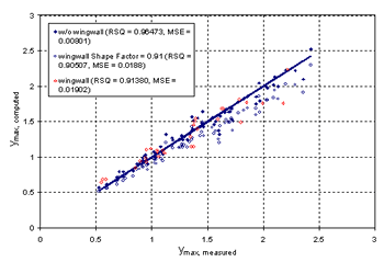
Figure 32. Measured and computed data with and without wingwalls, based on figure 31 regression.
Incorporating the adjustment function from figure 31 leads to the general equation:
 (39) where:
| KWW | = 1.0 for vertical face entrances
= 0.91 for wingwall entrances |
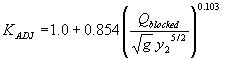
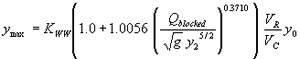
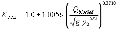
The fourth independent regression variable tested was the blocked discharge normalized by the acceleration of gravity (g) and the computed equilibrium depth. The R2 values were 0.07 for the vertical face data and 0.002 for the wingwall data (figures 33 and 34, respectively).
Figure 33. Maryland DOT's (Chang's) resultant velocity with Chang's approximation equation and local scour ratio as a function of the blocked discharge normalized by the acceleration of gravity (g) and the computed equilibrium depth.
Figure 34. Measured and computed data with and without wingwalls, based on figure 33 regression.
Using the adjustment function from figure 33 gives the general equation:
 (40) where:
| KWW | = 1.0 for vertical face entrances
= 0.89 for wingwall entrances |
Table 1 below gives an overview for the tested independent regression variables and R2 values using the Maryland DOT (Chang) method for representative velocity and critical velocity.
Table 1. Independent regression variables and R2 values using the Maryland DOT (Chang) method.
| Maryland DOT (Chang) Method for VR and VC |
R2 Regression |
R2 Meas. vs. Comp |
Equation No. |
|---|
 | 0.2150 | 0.9630 | (41) |
 | 0.2295 | 0.9658 | (42) |
 | 0.1865 | 0.9594 | (43) |
 | 0.0045 | 0.9491 | (44) |
 | 0.2891 | 0.9647 | (45) |
 | 0.0639 | 0.9427 | (46) |
GKY Method for Representative Velocity and Maryland DOT (Chang) Method
for Critical Velocity
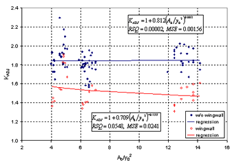
Two different independent regression variables were examined for this combination. Again, the approach flow area that is blocked by the embankments on one side of the channel over the squared flow depth was used as the independent regression variable, which gave R2 values of 0.00002 for the vertical face data and 0.05 for the wingwall data (figures 35 and 36, respectively).
Figure 35. GKY's resultant velocity with Chang's approximation equation for the critical velocity and local scour ratio as a function of the blocked area over the squared flow depth.
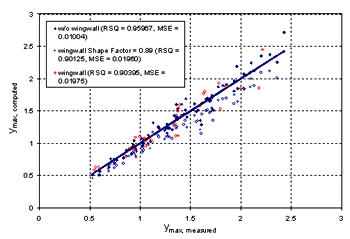
Figure 36. Measured and computed data with and without wingwalls, based on figure 37 regression.
The general equation can be formulated by inserting KADJ from figure 35:
 (47) where:
| KWW |
= 1.0 for vertical face entrances
= 0.89 for wingwall entrances |
The second independent regression variable tested for this combination was the blocked area over the squared computed equilibrium depth. The R2 values were 0.30 for the vertical face data and 0.06 for the wingwall data (figures 37 and 38, respectively).
Figure 37. GKY's resultant velocity with Chang's approximation equation for the critical velocity and local scour ratio as a function of the blocked area over the
squared computed equilibrium depth.
Figure 38. Measured and computed data with and without wingwalls, based on figure 37 regression.
Incorporating the adjustment function from figure 37 leads to the general equation:
 (48) where:
| KWW | = 1.0 for vertical face entrances
= 0.92 for wingwall entrances |
Table 2 gives an overview for the tested independent regression variables and R2 values using the GKY method for representative velocity and the Maryland DOT (Chang) method for critical velocity.
Table 2. Independent regression variables and R2 values using the GKY and Maryland DOT (Chang) methods.
| GKY Method for VR, Maryland DOT (Chang) Method for VC |
R2 Regression |
R2 Meas. vs. Comp. |
Equation No. |
|---|
 | 0.00002 | 0.9596 | (49) |
 | 0.2987 | 0.9715 | (50) |
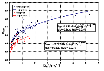
GKY Method for Representative Velocity and Critical Velocity
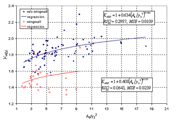
Three independent regression variables were tried using the GKY method for representative velocity and the GKY method for critical velocity, which is a combination of the SMB equations. Starting again with the approach flow area that is blocked by the embankments on one side of the channel over the squared flow depth as the independent regression variable results in R2 values of 0.50 for the vertical face data and 0.41 for the wingwall data (figures 39 and 40, respectively).
Figure 39. GKY's resultant velocity with the SMB equation for critical velocity and local scour ratio as a function of the blocked area over the squared flow depth.
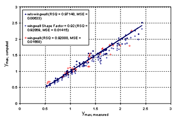
Figure 40. Measured and computed data with and without wingwalls, based on figure 39 regression.
Incorporating the adjustment function from figure 39 leads to the general equation:
 (51) where:
| KWW | = 1.0 for vertical face entrances
= 0.87 for wingwall entrances |
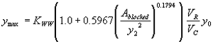
The blocked area over the squared computed equilibrium depth was used as the second independent regression variable. The R2 values were 0.78 for the vertical face data and 0.38 for the wingwall data (figures 41 and 42, respectively).
Figure 41. GKY's resultant velocity with the SMB equation for critical velocity and local scour ratio as a function of the blocked area over the squared computed equilibrium depth.
Figure 42. Measured and computed data with and without wingwalls, based on figure 41 regression.
Incorporating the adjustment function from figure 41 leads to the general equation:
 (52) where:
| KWW | = 1.0 for vertical face entrances
= 0.89 for wingwall entrances |
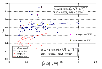
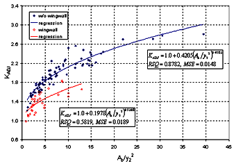
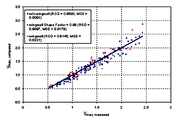
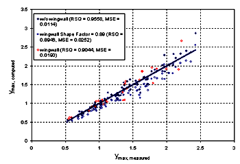
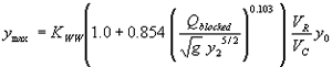
Testing the blocked discharge normalized by the acceleration of gravity (g) and the computed equilibrium depth as the independent regression variable yielded the best results. The R2 values were 0.84 for the vertical face data and 0.47 for the wingwall data (figures 43 and 44, respectively).
Figure 43. GKY's resultant velocity with the SMB equation for critical velocity and local scour ratio as a function of the blocked discharge normalized by the acceleration of gravity (g) and the computed equilibrium depth.
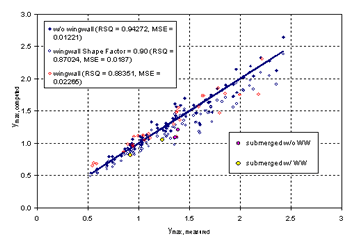
Figure 44. Measured and computed data with and without wingwalls, based on figure 43 regression.
Incorporating the adjustment function from figure 43 leads to the general equation:
 (53) where:
| KWW | = 1.0 for vertical face entrances
= 0.89 for wingwall entrances |
Table 3 below summarizes the results for the tested independent regression variables and R2 values using the GKY method for representative velocity and the SMB equation for critical velocity.
Table 3. Independent regression variables and R2 values using the GKY method for representative velocity and critical velocity.
| GKY Method forVR, SMB Equations for VC |
R2 Regression |
R2 Meas. vs. Comp. |
Equation No. |
|---|
 | 0.2883 | 0.8806 | (54) |
 | 0.8782 | 0.9690 | (55) |
 | 0.8621 | 0.9558 | (56) |
RIPRAP RESULTS
For the riprap analysis, the Maryland DOT (Chang) and GKY methods for computing representative velocity were used to calculate the effective velocity that accounts for turbulence and vorticity in the mixing zone at the upstream corner of a culvert. Two independent regression variables were used for the blocked area over the squared flow depth and the blocked discharge normalized by the acceleration of gravity (g) and the flow depth to compute the adjustment coefficient KRIP.
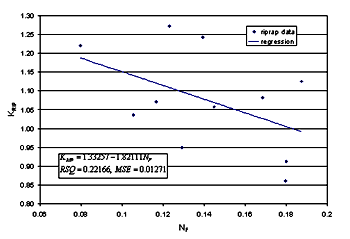
Maryland DOT (Chang) Method for Representative Velocity
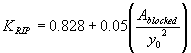
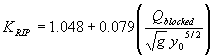
Using Chang's approximation equation for representative velocity and the approach flow area that is blocked by the embankments on one side of the channel over the squared flow depth to regress the effective velocity gives an R2 value of 0.39 (figures 45 and 46).
Figure 45. Maryland DOT's (Chang's) resultant velocity and stable riprap size from the Ishbash equation with the blocked area over the squared flow depth as the independent regression variable.
Figure 46. Measured and computed data, based on figure 45 regression.
The expression for sizing riprap at the upstream corners to protect bottomless culvert footings from scour is:
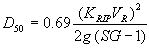 (57)
 (58) from figure 45.
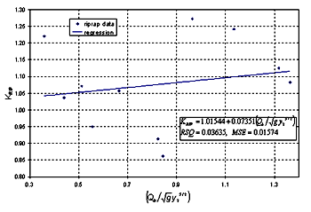
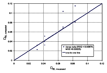
Testing the blocked discharge normalized by the acceleration of gravity (g) and the flow depth as the independent regression variable leads to a regression coefficient, R2, value of 0.036 (figures 47 and 48).
Figure 47. Maryland DOT's (Chang's) resultant velocity and stable riprap size from the Ishbash equation with the blocked discharge normalized by the
acceleration of gravity (g) and the flow depth as the independent regression variable.
Figure 48. Measured and computed data, based on figure 47 regression.
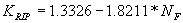
According to figure 47, the adjustment function for KRIP is:
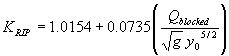 (59) Equation 59 can be substituted into equation 57 for the expression for sizing riprap.
Table 4 gives an overview of the tested independent regression variables and R2 values using Maryland DOT's (Chang's) representative velocity equations.
Table 4. Independent regression variables and R2 values using the Maryland DOT (Chang) method for representative velocity.
| Maryland DOT (Chang)Method for VR |
R2 Regression |
R2 Meas. vs. Comp. |
Equation No. |
|---|
| 0.2217 | 0.7357 | (58) |
| 0.0363 | 0.8367 | (59) |
GKY Method for Representative Velocity
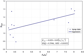
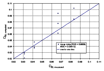
Computing the GKY method for representative velocity and the approach flow area that is blocked by the embankments on one side of the channel over the squared flow depth to determine the effective velocity gives an R2 value of 0.39 (figures 49 and 50).
Figure 49. GKY's resultant velocity and stable riprap size from the Ishbash equation with the blocked area over the squared flow depth as the independent regression variable.
Figure 50. Measured and computed data, based on figure 49 regression.
As indicated in figure 49, the regression analysis leads to:
 (60) Inserting equation 60 into equation 57 yields the expression for sizing riprap.
Finally, the blocked discharge normalized by the acceleration of gravity (g) and the flow depth as the independent regression variable was tested, resulting in a regression coefficient, R2, value of 0.04 (figures 51 and 52).
Figure 51. GKY's resultant velocity and stable riprap size from the Ishbash equation with the blocked discharge normalized by the acceleration of gravity (g)
and the flow depth as the independent regression variable.
Figure 52. Measured and computed data, based on figure 51 regression.
As shown in figure 51, the regression coefficient function is:
 (61) To gain the expression for sizing riprap, equation 61 may be substituted into equation 57.
Table 5 is an overview of the computed independent regression variables and their R2 values when using GKY's representative velocity to account for turbulence and vorticity in the mixing zone at the upstream corner of a culvert.
Table 5. Independent regression variables and R2 values using the GKY method for representative velocity.
| GKY Method for VR |
R2 Regression |
R2 Meas. vs. Comp. |
Equation No. |
|---|
| 0.3946 | 0.9009 | (60) |
| 0.0404 | 0.8348 | (61) |
Previous | Table of Contents | Next
|