U.S. Department of Transportation
Federal Highway Administration
1200 New Jersey Avenue, SE
Washington, DC 20590
202-366-4000
Federal Highway Administration Research and Technology
Coordinating, Developing, and Delivering Highway Transportation Innovations
 |
| This report is an archived publication and may contain dated technical, contact, and link information |
|
Publication Number: FHWA-RD-02-078 Date: November 2003 |
Bottomless Culvert Scour Study: Phase I Laboratory Report3. THEORETICAL BACKGROUNDAs the photographs in the previous section illustrate, the scour was always deepest near the corners at the upstream entrance to the culvert. This observation is attributed, in part, to the concentration of flow near the upstream corners as the flow that is being blocked by the embankments is contracted and forced to go through the culvert opening. However, it is also attributed to the vortices and strong turbulence generated in the flow separation zone as the blocked flow mixes with the main channel flow at the upstream end of the culvert (figure 10). It is much like the abutment scour phenomenon that researchers have observed for bridge scour models. 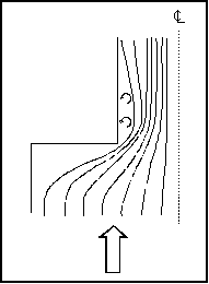 Figure 10. Flow concentration and separation zone. Several researchers, including Chang,(1) GKY and Associates, Inc.,(2) and Sturm,(3) have suggested that bridge abutment scour can be analyzed as a form of flow distribution scour by incorporating an empirical adjustment factor to account for vorticity and turbulence. The equilibrium flow depth required to balance the sediment load into and out of the scour zone for the assumed flow distribution can be determined analytically. The adjustment factor to account for vorticity and turbulence can be derived from laboratory results. These notions were used to formulate the theoretical background for analyzing the culvert scour data. Variables used in the data analysis are illustrated in the definition sketches (figures 11(a) through 11(c)). 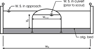 Figure 11(a). Definition sketch prior to scour. 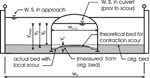 Figure 11(b). Definition sketch after scour. 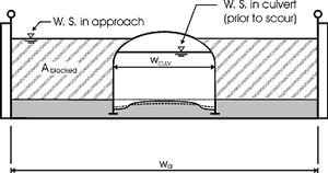 Figure 11(c). Definition sketch for blocked area. Equation 2 is an expression for the unit discharge for an assumed flow distribution remaining constant as the scour hole develops. If no sediment is being transported into the scour hole, as was the case with all of our experiments, then no sediment can be transported out of the scour hole at equilibrium. In this case, the velocity must be reduced to the critical incipient motion velocity for the sediment size at the equilibrium flow depth (y2). This equation forms the basis for the analysis: where: VRY0 = qR = the assumed representative unit discharge across the scour hole at the beginning of scour The above equation can be rearranged to yield an equilibrium flow depth (y2) after the representative velocity (VR) at the beginning of scour and the critical incipient motion velocity (VC) are determined. This equilibrium depth reflects the scour that is attributed to the flow distribution. The measured maximum depth at the corners of the culvert was always greater than the computed equilibrium depth. An empirical coefficient (KADJ), defined by equation 3, was needed to explain the extra scour depths. The laboratory data and regression analyses were used to derive an expression for this coefficient. Several different independent variables were tried to derive the expression for KADJ; however, what seemed to work best for this data was the blocked discharge (Qblocked) normalized by the acceleration of gravity (g) and the computed equilibrium depth (y2) as formulated in equation 4: 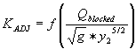 (4) (4)Qblocked is the portion of the approach flow to one side of the channel centerline that is blocked by the embankment as the flow approaches the culvert. The literature describes several methods for determining an approximation for representative velocity and critical velocity. Methods described by Chang and by GKY were tried in various combinations to determine which worked best for this data. These methods are discussed below. CALCULATING REPRESENTATIVE VELOCITYMaryland DOT (Chang) Method for Representative Velocity Chang, through his work for the Maryland SHA, developed equations 5 and 6 to calculate the resultant velocity based on potential flow assumptions at a distance equal to one-tenth of the length of the blocked flow (figure 12): 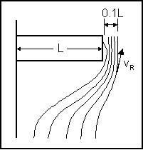 Figure 12. Chang's resultant velocity location. 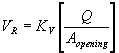 (5) (5)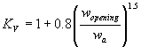 (6) (6)where:
These equations are dimensionally homogeneous and are independent of the system of units as long as they are consistent. GKY Method for Representative Velocity GKY describes representative velocity across the scour hole as the resultant of the lateral and longitudinal velocity components as shown in equations 7, 8, and 9. Applying the Pythagorean theorem yields: with It should be noted that equation 9 above is an unpublished modification of the method published by Young, et al.(2); however, the basic concept is similar to the published version. For the simple rectangular cross section used for the flume experiments, Qblocked could be estimated from equation 10:
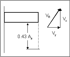 Figure 13. GKY's resultant velocity approach. NUMERICAL MODEL FOR CALCULATING REPRESENTATIVE VELOCITYSince some designers probably have access to 2D numerical models, they will not necessarily need to rely on the 1D approximations for representative velocity to be used in the computations. Xibing Dou simulated the laboratory experiments with a 2D numerical model. This model uses the Finite Element Surface-Water Modeling System: Two-Dimensional Flow in a Horizontal Plane (FESWMS-2DH) program to solve the hydrodynamic equations that describe 2D flow in the horizontal plane. The effects of bed friction and turbulent stresses are considered and water column pressure is hydrostatic. The estimation of representative velocity uses the average x and y element velocities ( 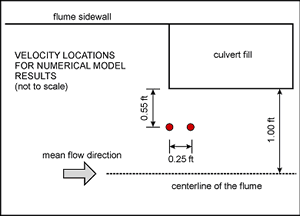 Figure 14. Velocity locations for 2D model. 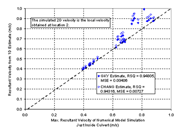 RSQ = R2 = correlation coefficient Figure 15 is a comparison of the 2D numerical model results with the 1D approximations suggested by Chang and GKY. The 1D approximations are consistently higher than the numerical results, which is interpreted to mean that the 1D approximations are conservative. Numerical model results could underpredict scour if they are used with empirical equations based on 1D approximations; however, the differences are probably insignificant compared to the differences in the ideal conditions tested in the flume and the conditions that are in a natural channel. In addition to the previous comparison between numerical and 1D measurements, figure 16 shows the comparison between Chang's resultant velocity and GKY's resultant velocity. 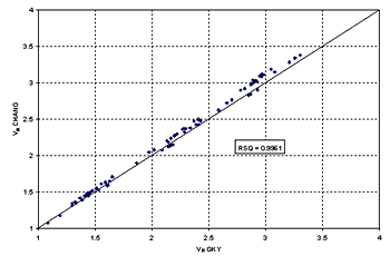 Figure 16. Comparison of Chang's and GKY's resultant velocities. CALCULATING CRITICAL VELOCITYMaryland DOT (Chang) Method for Critical Velocity Chang uses Niell's(4) competent velocity curves to calculate critical velocity. Niell presents a set of competent (critical) velocity curves based on flow depth, velocity, and the size of the bed material. Niell's curves are derived from the Shields curve using varying Shields numbers for different particle sizes. To facilitate doing computations on a computer spreadsheet, Chang(2) derived a set of simplified equations that represent Niell's curves quite well. Niell's Competent Velocity Concept Niell's competent velocity is comparable in its definition to the critical flow velocity for causing incipient motion of bed materials. The equations by Laursen and Niell for computing critical velocity (presented in FHWA's Hydraulic Engineering Circular 18 (HEC-18)) are generally applicable for particles of bed material larger than 0.03 m (0.1 ft). For bed material smaller than this size, these equations can be expected to underestimate critical velocity. Niell developed a series of curves for determining the critical velocity for particles smaller than 0.03 m based on the Shields curve. Chang transformed the plots of Niell's curves (figure 17) into a set of equations for computing critical velocity based on the flow depth and the median diameter of the particle. These equations are set forth below. 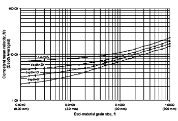 Figure 17. Competent velocity curves for the design of waterway openings in scour backwater conditions (from Niell).(4)
The exponent x is calculated using equation 13: where:
where:
Chang's equations are plotted in figure 18. Niell's competent velocity curves are intended for field conditions with flow depths of 1.5 m (5 ft) or greater. Chang's equations were extrapolated to flow depths below 0.30 m for these experiments and to curves for flow depths of 0.305 and 0.15 m (1 and 0.5 ft) (figure 18). Our sediment sizes fell in a range that could be described by equations 12 and 13. 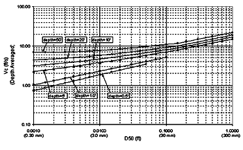 1 ft = 0.305 m
Figure 18. Chang's approximations. GKY Method for Critical Velocity The GKY method combines the Shields,(5) Manning,(6) and Blodgett(7) (SMB) equations to calculate critical velocity. The starting equation is the average shear stress in a control volume of flow: Experimental observations highlighted the importance of the Shields parameter (SP), which is defined as: The critical value of the stability parameter may be defined at the inception of bed motion, i.e., SP=(SP) c=0.047. Shields showed that (SP)c is primarily a function of the shear Reynolds number (figure 19). 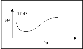 Figure 19. Shields parameter as a function of the particle Reynolds number. Rearranging equation 16, inserting (SP)c = 0.047, and setting Rearranging Manning's equation to compute the friction slope leads to: 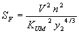 (18) (18)where:
Substituting equation 18 for SF in equation 17 results in: This may be simplified by consolidating the specific weight Note that: Sand such as that used in these experiments is considered to have a specific gravity (SG) of 2.65. Substituting this into equation 20 and rearranging to isolate VC2 leads to: The square root of equation 22 gives the equation for computing critical velocity: Blodgett's equations for average estimates of Manning's n for sand- and gravel-bed channels follow. Equation 25 applies for the depths and sand particle sizes used in our experiments. 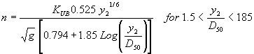 (24) (24)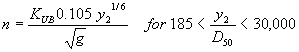 (25) (25)
Substituting equation 25 for n in equation 23 and then simplifying leads to: 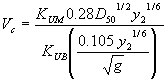 (26) (26)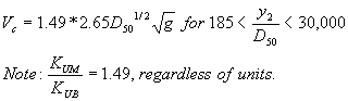 (27) (27)Equation 27 is dimensionally homogenous and does not require a units conversion. Combined Competent Velocity Curves To give an overview of how the different competent (critical) velocity methods behave, the critical velocity equations for various particle sizes were plotted for 3- and 0.305-m (10- and 1.0-ft) flow depths (figures 20 and 21). Comparing the two plots, the SMB velocity curve drifts away from Chang's approximation and Niell's competent velocity curve for the 3-m (10-ft) flow depth. For a flow depth of 0.305 m (1 ft), this is not the case, which confirms both methods for critical velocity estimation since the experiments were performed in this flow-depth range. 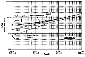 1 ft = 0.305 m
Figure 20. Combined competent velocity curves for a flow depth of 3 m (10 ft). 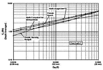 1 ft = 0.305 m
Figure 21. Combined competent velocity curves for a flow depth of 0.3 m (1.0 ft). SCOUR PROTECTION TASK: RIPRAP ANALYSISMany researchers have developed critical conditions based on average velocity. Ishbash(8) presented an equation that can be expressed as: Ishbash described two critical conditions for riprap stability. For loose stones where no movement occurs, NSC is expressed as: 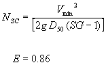 (29) (29)For loose stones allowed to roll until they become "seated", NSC is expressed as: 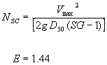 (30) (30)where:
Equation 30 for riprap that will just begin to roll can be written as equation 31. For the culvert experiments, we represented the effective velocity (Veff) in terms of an empirical multiplier as indicated by equation 32, which is substituted into equation 31 to yield equation 33. 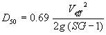 (31) (31)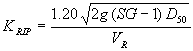 (33) (33)where:
Equations 31 through 33 are dimensionally homogeneous and can be used with either system of units as long as they are consistent. Regression analysis was then performed to derive a function for the coefficient KRIP. |

