• Federal Highway Administration >
• Publications >
• Research Publications >
• Hydraulics Publications >
• 05072 >
• 02.Cfm >
• Assessing Stream Channel Stability At Bridges in Physiographic Regions

Assessing Stream Channel Stability At Bridges in Physiographic Regions

2. BACKGROUND AND LITERATURE REVIEW

A healthy, stable stream is resilient to disturbances, such as the passing of storm events and changes induced by humans. Dimensions of the stable stream channel are sustainable over decades. There is variability in roughness, which is important to ecological diversity. The stable stream is characterized by healthy, upright, woody vegetation; low banks that are not susceptible to mass wasting (gravity failures); and a flood plain that is connected to the river. Thus, during moderate flow events, the flood plain is active. Figure 1 provides an example of a stable stream. On the other hand, an unstable stream is characterized by overheightened, oversteepened banks that are susceptible to mass wasting, evidence of geotechnical failure planes along the banks, lack of diverse, upright woody vegetation, and the flood plain is disconnected from the channel so that moderate to high flows remain within the channel banks. Thus, wetlands tend to drain, and the nutrient source to the stream is cutoff. Figure 2 provides an example of an unstable stream channel.

Thorne et al.categorize alluvial channel stability as unstable, stable-dynamic, or stable-moribund. (7) They defined an unstable channel as one where degradation, aggradation, width adjustment, or planform changes were actively occurring in time and space. However, the main requirement is that there is net morphological change over engineering time scales. A dynamically stable channel is defined by Thorne et al.as one in which the characteristic dimensions do not change over engineering time scales. (7) Thorne et al. also define a moribund channel as one in which the characteristic dimensions have been formed by a prior flow regime different from that which is presently observed, or more likely, due to channel widening and dredging in low energy rivers. (7) Moribund channels are unlikely to recover from past engineering activity even if allowed to do so, because the river is unable to mobilize its bed material.

Brookes inferred channel stability in terms of stream power. (11) Based on field observations of stable and unstable streams in the United Kingdom, he found that in unconfined lowland, meandering channels—streams in which the stream power at bankfull discharge was greater than about 35 watts per square meter (W/m²)—were unstable in terms of erosive adjustment. In these channels where stream power was less than 25 W/m², the stream was stable. Although such guidance is certainly useful, it is often very difficult to define bankfull in an unstable channel. (12) In addition, the criterion developed by Brookes will only be valid in the region where he collected the observations.

Figure 1 . Stable stream in central Pennsylvania.

Figure 2 . Unstable stream in western Pennsylvania.

Chorley and Kennedy described stability in terms of three types of equilibrium: (1) static, in which a static condition is created by a balance in opposing forces; (2) steady-state, in which the properties of a stream randomly oscillate about a constant state; and (3) dynamic, in which a balanced state is maintained by dynamic adjustments. (13) Richards showed that in a natural, stable channel, channel dimensions constantly adjust to passing floods. (14) So, although a stable channel has constant average dimensions over a medium timeframe (on the order of decades), those dimensions vary about the average value. Figure 3 shows an example of variation in width over time about the average width.

Figure 3. Variation of channel width over medium timeframe about
the stable mean (after reference 14).

Knox defines a stable stream as "one in which the relationship between process and form is stationary and the morphology of the system remains relatively constant over time." (15) At bridges, stability also implies limited lateral movement so that the channel is more or less centered beneath the bridge opening. A geomorphically stable channel that has considerable lateral migration is likely to be considered unstable by the engineer concerned with bridge safety.

Channel stability must be defined in terms of both time and space. The temporal and spatial scales used vary depending on the application. Temporal scales for channel stability can range from medium, in which one might be concerned about bridge safety or ecological recovery, to long term, which would include geomorphic and geologic stability. A short timeframe is considered to be on the order of 1 or 2 years; medium is decades to 100 years, typical of engineering design lives; and long term is hundreds to thousands of years. Spatial scales can also vary widely depending on how stability is defined. Length of stream over which stability is determined can be as short as several hundred feet, to 20 stream widths (a rule-of-thumb established by Leopold), to miles of stream.

CHANNEL ADJUSTMENTS

Rivers become temporarily unstable when new hydrologic or sediment load conditions are imposed. (16) Lane described this process as a proportionality between the loads entering the stream: (17)

(1)

where Q_s = sediment discharge, d = sediment size, Q = water discharge, and S = slope. Thus, a change in either of the loads, Q_s or Q, will result in adjustments of sediment size or slope. Hey expanded on equation 1 by determining the dependent variables that will adjust according to changes in the independent variables of the equation. (18) The independent variables are sediment discharge, bed and bank sediment characteristics, water discharge, and valley slope; the dependent variables include velocity, mean flow depth, channel slope, width, maximum flow depth, bedform wavelength, bedform amplitude, sinuosity, and meander arc length.

Changes in the independent variables can be brought about by either natural events or

human-induced modifications. The changes can be direct or indirect. Natural events that increase sediment discharge include landslides and destabilization of channel banks by extreme hydrologic events. Water discharge is increased as storms and hurricanes create flooding in the stream channels and flood plains. Climatic changes also can gradually increase or decrease water discharge to a channel.

Human modifications to stream channels such as straightening, clearing, dredging, and widening can result in dramatic responses within the reach directly modified, as well as upstream or downstream of the modified reach. A good example of this is channel straightening. Straightening imposes an increased channel slope in the modified reach. To adjust to the new slope, a head cut often will proceed upstream, rapidly lowering the channel elevation. Many other modifications can affect the loads to a stream channel. Downstream of a dam, sediment discharge is decreased, typically resulting in bed degradation and a change in slope. Dams, other than run-of-the-river dams, also change the water discharge such that the discharge downstream is steadier at a higher discharge than for previous low flows. Larger events typically are stored in the reservoir. The result is downstream degradation due to maintaining a higher-than-normal flow over an extended period of time. Land use changes have significant, indirect impacts on channel adjustments. Deforestation for the purposes of either urbanization or agriculture often dramatically impact stream channels. Without woody vegetation, the banks become more susceptible to changes in discharge. Removing vegetation across the flood plain creates a reduced roughness and infiltration surface, thus increasing both the magnitude and timing of the flood hydrographs in the streams. This, in turn, increases movement of sediment in the river banks and bed. Construction during urbanization in a watershed increases fine sediment to a stream channel. Depending on the type of channel, this increase in sediment can change the channel morphology.

The response of a river to modifications in the sediment and water discharge depends on the type of channel and the type of modification. Changes in sediment or water discharges can occur as either a pulse or a step (chronic) change. (19) A pulse may result in a temporary channel adjustment, but then return to its previous equilibrium dimensions. However, a step change is more likely to result in a permanent change to the stream stability and equilibrium dimensions. The length of time over which the channel reaches its new equilibrium or returns to a previous state depends on the intensity of the change in load as well as the type of channel and its resilience. Montgomery and MacDonald provide tables of the relative sensitivity of alluvial channel types to chronic changes in coarse sediment, fine sediment, and discharge. (20) The channel types are cascade, step-pool, plane bed, pool-riffle, and dune-ripple. For each channel type, they determine sensitivity to change as very responsive, secondary or small response, and little or no response. In every case, pool-riffle streams are the most sensitive to changes in the load. Their dimensions (depth and width) and bank stability are very sensitive to changes in coarse sediment supply and to increases in discharge. Bed material in these channels is also very responsive to changes in sediment supply and water discharge. By comparison, cascade and step-pool channels are not as sensitive and will maintain their dimensions and bank stability under conditions of change in sediment and water supply.

CHANNEL STABILITY AT BRIDGES

Knowledge of the spatial and temporal trends of channel adjustments is central to protecting and maintaining bridges. One well-known bridge collapse due to stream channel instability is the U.S. Route 51 bridge over the Hatchie River in Tennessee. During a 3-year flood, this bridge collapsed, killing eight people. The collapse was caused by lateral channel migration of 25.3 m over 13 years. The rate of lateral migration had increased dramatically following channel straightening to reduce the angle at which the channel approached the bridge. There are many other examples of bridge failures following channel modifications. Straightening of the Willow River in southwestern Iowa led to channel bed degradation and gully formation, resulting in the need to repair and reconstruct roads and bridges in the area. (21) Straightening and dredging of the Homochitto River in southwest Mississippi and the Blackwater River in Missouri caused significant bed degradation and widening, and led to the collapse of several bridges. (22, 23) Additional bridge failures occurred in straightened western Tennessee channels as a result of channel bed degradation, channel widening, and local scour. (24, 25)

Channel instability in the vicinity of a bridge can be arrested through the use of bank and bed stabilization structures, but if they fail during a hydrologic event, the bridge is at risk again. As an example, in 1995, a railroad bridge near Kingman, AZ, collapsed as an Amtrak® train crossed it, injuring more than 150 people. The cause was the sudden upstream migration of a head cut during heavy rains. Before this hydrologic event, the head cut migration had been halted by a check dam. When the check dam failed during the storm, the head cut was free to travel upstream.

Several studies have been conducted to assess the reliability of bridges in which piers and/or abutments are in an unstable, adjusting stream. (26, 27) However, the key to assessing risk or reliability is identifying that a problem or potential for a problem exists and documenting the condition.

METHODS FOR COLLECTING STREAM CHANNEL DATA

Systematic data collection is an integral part of conducting a reconnaissance along a stream or assessing channel stability. The amount of data that is required depends on the level of detail desired. A wide range of data is useful in assessing stream channel conditions. The data include topographic maps, aerial photos, bridge inspection reports, hydrologic and hydraulic reports, stream gage data, and other geomorphic reports. Aerial photos and topographic maps are very useful in providing an overall view of the bridge, the stream below it, and the watershed conditions. Comparing photos and maps over a period of years is helpful in assessing rates of change, particularly at a larger scale. Both aerial photos and topographic maps can be viewed online at http://terraserver-usa.com. These tools help visualize the location of the bridge relative to the location of meanders, as well as the bridge alignment. Given the relative ease of checking aerial photos, this should be done as a standard part of any survey. In addition to studying photos and maps, examining previous reports on assessments conducted at or near the bridge is useful to determine trends. Given that bridge inspections are conducted at least every 2 years, typically with one or two cross sections measured, these are good reports to compare for changes over a longer period of time. Geomorphic assessments that have been conducted along the stream, although they may not be concerned with the bridge, are also excellent sources of information. HEC-20 details these types of data and where to access them. (3)

Collecting data along a stream to assess stream condition can include a wide variety of data and levels of detail. Thus, a systematic method of collection is essential to producing consistent data sets that can be compared and used for future analyses. The only complete, systematic, geomorphic data collection system that exists today is that created by Thorne. (2) In this system, multiple pages of forms provide a systematic methodology for collection of data and subjective observations. Data collection begins with geological and watershed level observations, then continues to focus on the stream corridor and hill slopes, and finally examines the actual bed and banks of the channel or water body. The data set developed through this reconnaissance provides complete documentation of current conditions. In addition, photographs are taken to help document current conditions. The Thorne reconnaissance method does not address infrastructure within a reach; thus, it is necessary to add parameters for that case. Johnson et al.revised the Thorne data sheets to suit streams in urban environments and provide descriptions of conditions at instream structures. (28) The data collected included descriptions of the valley, channel, bed sediment, bank material, vegetation, erosion, flood plain, instream structures, and reach measurements. According to Thorne, a reconnaissance could range from a very detailed study over 5–10 river widths that would include 1 pool-riffle couplet, individual meander, primary bifurcation-bar-confluence unit in braided channel, to a low level detail study over a much longer reach in which channel form and processes do not change significantly. (2)

The NHI training course on bridge scour and stream stability has emphasized the use of reconnaissance sheets developed by Thorne for systematically collecting geomorphic data. (3) The sheets are divided into five sections, with each section further divided into parts that focus on various aspects of the stream. These can be summarized as:

• Section 1—Scope and Purpose, including general information on the location and details of the project.
• Section 2—Region and Valley Description, including descriptions of the area around the river valley, river valley and valley sides, flood plain, vertical relation of channel to valley, and lateral relation of channel to valley.
• Section 3—Channel Description, including a description of the channel dimensions, controls, bed materials, and bar types and materials.
• Section 4—Left Bank Survey, including bank characteristics, vegetation, bank erosion, geotechnical failures, and toe sediment accumulation of the left bank.
• Section 5—Right Bank Survey, including bankcharacteristics, vegetation, bank erosion, geotechnical failures, and toe sediment accumulation of the right bank.

The method also includes numerous entries for subjective or interpretive observations. Bridge abutments and armor protection are entered on the data sheets as obstructions. Although individual items on the data sheets may not indicate channel stability or instability directly, the data are collectively important in assessing long-term stability. Table 1 provides the relationships between the data collected in Thorne's reconnaissance and long-term indications of stability. These relationships provide impetus for the development of the simplified reconnaissance sheets in terms of using the stability assessment method described in this report.

CHANNEL STABILITY ASSESSMENT METHODS

A number of methods currently are available for assessing channel stability. Some require the expertise of an experienced geomorphologist, while others require only a brief period of training. All of these methods are, at least in part, based on observations of a variety of parameters that describe the characteristics and conditions of the channel and surrounding flood plain. The purpose of each of these methods is to assess the current condition of the channel and possibly identify the processes that are acting to change the condition over at least a reach level or over the entire watershed system. The goal of the assessments is to better understand the processes so that stream restoration, bank stabilization, or a host of other river applications can be designed successfully. These methods are discussed briefly below.

Pfankuch developed a method to rate stream stability for mountain streams in the northwestern United States. (5) The methodology was developed for the purpose of planning various stream projects on second- to fourth-order streams. The user evaluates the condition of the stream by assessing 15 stability indicators. For each indicator, the user rates the stream reach as excellent, good, fair, or poor based on a set of qualitative descriptions for each category. Each indicator and rating is associated with a number of points. When the ratings have been completed, the points are added to yield a total score. The total score is then related to a subjective description for the overall stability of the stream as excellent, good, fair, or poor; the higher the number, the more unstable the stream. The following list of parameters is used to indicate stability: bank slope, mass wasting, debris jam potential, vegetative bank protection, channel capacity (includes width-to-depth ratios), bank rock content, channel obstructions, bank cutting, deposition, angularity of rocks on bed, brightness of rocks, consolidation of bed material, bed material size, scouring, and moss and algae present. Thorough descriptions of each parameter are provided. The use of several of these parameters to infer stability is questionable. For example, brightness is used to describe the polishing of rocks, presumably due to movement. If less than 5 percent of the bottom is "bright," then the brightness is rated as excellent; if 5 to 35 percent of the bottom is "brighter" than the rest, then it is rated good, and so on. Not only is this a difficult parameter to evaluate, but also it would be highly variable in meaning from one stream to the next. The use of channel capacity to assess stability is also very subjective and problematic. In this method, the rating is excellent if the width-to-depth ratio, w/y, is less than 7, the cross section is ample for present peak volumes, and out-of-bank floods are rare. This may not be an appropriate rating, since the combination of w/y is less than 7 and "rare" bank floods may indicate an incising, unstable channel.

HEC-20is a manual for bridge owners and inspectors to assess channel stability and potential stability-related problems in the vicinity of bridges and culverts. (3) A suggested three-level approach covers: (1) geomorphic concepts and qualitative analysis; (2) hydrologic, hydraulic, and sediment transport concepts; and (3) mathematical or physical modeling studies. If the results of level 1 suggest that the channel may be unstable in either the vertical or lateral direction, then the user is guided to continue to level 2. Based on those results, the user may or may not be instructed to continue to level 3. Level 1 is the qualitative analysis of geomorphic conditions leading to instability. Therefore, the details of this level will be described here. In level 1, the user completes a six-step process to determine the lateral and vertical stability and the potential response of the channel to changes. Step 1 is the collection of geomorphic data, such as stream size, flow habit, bed material, valley setting, flood plain and levee description, incision, channel boundaries, bank vegetation, sinuosity, braiding, and bar development. Each of these indicators is described in HEC-20. Step 2 involves reviewing historic changes in land use. Step 3 requires an assessment of overall stability based on data collected in step 1 as well as additional factors, such as dam and reservoir location, head cuts, sediment load, bed material size, flow velocity, and stream power. In step 4, lateral stability is evaluated as highly unstable, moderately unstable, or stable based on bank slope, bank failure modes, bank material, vegetation, and historic channel migration. In step 5, vertical channel stability is evaluated based on historic gradation changes and site observations. Finally, in step 6, the channel response to changes in sediment discharge, flow rate, bed slope, and sediment size is predicted.

Johnson et al.developed a rapid stability assessment method based on geomorphic and hydraulic indicators. (1) This method has been included in the most recent revision of HEC-20. It can be used within HEC-20 as a method to provide a semiquantitative level 1 analysis and to determine whether it is necessary to conduct a more detailed level 2 analysis. Thirteen qualitative and quantitative stability indicators are rated, weighted, and summed to produce a stability rating for gravel bed channels. It was based largely on previous assessment methods. (5,6, 7) The primary limitation of the method is that it was developed and tested only in the Piedmont and glaciated Appalachian Plateau regions of Maryland and Pennsylvania.

Mitchell (29) and Gordon et al. (30) describe qualitative reconnaissance type surveys to assess stability of streams in Victoria, Australia. Field evaluations at each site typically were completed in only a few hours due to the nature of the sampling. Much of the sampling was completed by comparing the reach conditions to a set of drawings to categorize bank shape, channel shapes, bed material, and types and shapes of bars. However, criteria such as bank stability and bed aggradation or degradation were omitted from the data collection process due to the inconsistency of that information. The parameters that were evaluated and rated as very poor, poor, moderate, good, and excellent with respect to stability were bed composition, proportion of pools and riffles, bank vegetation, verge (riparian) vegetation, cover for fish, average flow velocity, water depth, underwater vegetation, organic debris, and erosion/sedimentation. The ratings for each parameter were based on qualitative descriptions. An overall rating then was assigned to each site based on the ratings of the 10 variables listed. However, the method used to determine the overall rating was not discussed.

Based on previous work by Simon, (24) Simon and Downs (6) developed a method for assessing stability of channels that have been straightened. In this method, a field form is provided for data collection in a 1.5- to 2-hour period. The data then are summarized on a ranking sheet. For each category on the ranking sheet, a weight is assigned where the value of the weights was selected based on the authors' experience. A total rating is derived by summing the weighted data in each category. The higher the rating, the more unstable the channel is. Simon and Downs found that for streams in western Tennessee, a rating of 20 or more indicated an unstable channel that could threaten bridges and land adjacent to the channel. (6) The rating system provides a systematic method for evaluating stability; however, the final ratings cannot be compared to streams evaluated in other geomorphic, geologic, or physiographic regions. In addition, some of the parameters are very difficult to assess, particularly in the absence of a stream gage. For example, considerable weight is placed on identifying the stage of channel evolution. To properly assess this stage, it is necessary to determine whether the channel is in the process of widening, degrading, or aggrading. Simon and Hupp provide a good description of determining bed degradation based on gage data. (31) However, determining aggradation or degradation based on a gage analysis typically requires at least several years of stream gage data. (3) Simon and Downs also have included rating information for bridges in the reach; this information can be used for geomorphic instabilities in the vicinity of the bridge, but does not incorporate local instabilities, such as bridge scour. (6)

Thorne et al.expanded on the method developed by Simon and Downs by adding a quantitative segment based predominantly on hydraulic geometry analysis. (7) The ranking based on the Simon and Downs method provides a qualitative assessment, while comparing measured hydraulic geometry to that calculated from equations developed for stable channels provides a quantitative measure of stability. A set of hydraulic geometry equations was assembled for gravel bed rivers, and the use was demonstrated on an actual river. The observed width and depth of a stream reach were compared to the regime width and depth calculated from the hydraulic geometry equations. Significant differences can then be assumed to imply that the observed channel is either in regime, or it is not. Although this is a reasonable approach, hydraulic geometry equations must be used cautiously because they are derived empirically. In addition, Merigliano showed that hydraulic equations do not always reflect channel behavior because of variability in other important parameters, such as turbulence, sediment distribution, and velocity distribution, that are not included in the equations. (32) Therefore, while it may be useful to use hydraulic geometry equations as a check on stability, the equations imply a level of accuracy and applicability that may not be appropriate. The qualitative and quantitative information is then assembled into a one-page report that summarizes the state of the channel stability. Writing the summary requires a great deal of field experience, because it is necessary to draw inferences from the qualitative and quantitative data.

In an attempt to reduce the amount of time required for a full geomorphologic study, Fripp et al.developed a stream stability assessment technique based on a one-page field form. (33) The required data to be collected include a basic description of the reach; restoration potential (or needs); channel bed condition in terms of whether it is stable, aggrading, or degrading; grade and bank controls; debris jams present; bank cover; bank erodibility (in terms of low, medium, or high); riparian buffer width; channel bed material; and cross-sectional measurements. From the collected data, it is suggested that the assessor rate the channel stability as good, fair, bad, or very bad based on qualitative descriptions of the channel bed and bank. It is not clear how all of the data collected on the field form are used in making the assessment. The authors stress that the stability assessment be based on the stream condition, not on any structures crossing the stream.

Myers and Swanson (34, 35) applied the method developed by Pfankuch (5) to assess and monitor stream channel stability for streams in northern Nevada. They correlated the stream stability ranking to the stream type according to the Rosgen classification scheme. (36) Myers and Swanson found that several of the stability indicators proposed by Pfankuch were not useful in the evaluation. Based on these findings, they deleted rock angularity from the rating procedure and separated the combined scour and deposition indicator into two individual indicators. They also made slight adjustments to the scoring procedure. In addition, they found that if the rating was combined with a stream classification, the underlying morphological processes could be inferred from the classification, which then could be used to indicate an appropriate engineering response to mitigate further stream instability.

Montgomery and MacDonald suggest a diagnostic approach in which the system and system variables are defined, observations are made to characterize the condition of the system, and an evaluation is made to assess the causal mechanisms producing the current condition. (20) Observations are based on characterizing both the valley bottom and the active channel according to a set of field indicators. Valley bottom indicators include the channel slope, confinement, entrenchment, riparian vegetation, and overbank deposits. Indicators for the active channel include the channel pattern, bank conditions, gravel bars, pool characteristics, and bed material.

Rosgen proposed a channel stability assessment method that is based on assessing stability for a stable reference reach, then assessing the departure from the stable conditions on an unstable reach of the same stream type. (37) The stability analysis consists of 10 steps that assess various components of stability. The steps include measuring or describing: (1) the condition or "state" categories (riparian vegetation, sediment deposition patterns, debris occurrence, meander patterns, stream size or order, flow regime, and alterations); (2) vertical stability in terms of the ratio of the lowest bank height in a cross section divided by the maximum bankfull depth; (3) lateral stability as a function of the meander width ratio and the bank erosion hazard index (BEHI); (4) channel pattern; (5) river profile and bed features; (6) width-to-depth ratio; (7) scour and fill potential in terms of critical shear stress; (8) channel stability rating using a modification of the Pfankuch (5) method; (9) sediment rating curves; and (10) stream type evolutionary scenarios. This is a very data-intensive assessment method and not one that bridge inspectors or hydraulic engineers will likely use, due to the time and expense of data collection. However, one of the more interesting components of this method is the procedure for step 8. Like the Pfankuch method, a rating of good, fair, or poor is obtained based on a numerical rating. However, Rosgen modified the method to account for differences across the 42 different stream types, so that each stream type has a separate definition for good, fair, and poor. For example, a rating of 60 would be considered poor in a B1 stream, fair in a C1 stream, and good in an F1 stream. Although the approach is interesting and has merit, the basis for the 42 separate rating schemes is not given.

USACE suggests a three-level stability analysis for the purpose of stream restoration design. (10, 38) Level 1 is a geomorphic assessment, level 2 is a hydraulic geometry assessment, and level 3 is an analytical stability assessment that includes a sediment transport study. As part of the geomorphic assessment, USACE recommends collecting the following field data: watershed development and land use, flood plain characteristics, channel planform, and stream gradient; historical conditions; channel dimensions and slope; channel bed material; bank material and condition; bedforms, such as pools, riffles, and sedimentation; channel alterations and evidence of recovery; debris and bed and bank vegetation; and photographs. Indicators of channel degradation are given as terraces, perched channels or tributaries, head cuts and knickpoints, exposed pipe crossings, perched culvert outfalls, undercut bridge piers, exposed tree roots, leaning trees, narrow and deep channels, undercut banks on both sides of the channel, armored beds, and hydrophytic vegetation located high on the banks. Indicators of a stable channel include vegetated bars and banks, limited bank erosion, older bridges, culverts and outfalls with inverts at or near grade, no exposed pipeline crossings, and tributary mouths at or near existing main stem stream grade. Copeland et al. further suggest that spatial bias in assessing stability can be reduced by walking a distance well upstream and downstream of the project reach, while temporal bias can be reduced by revisiting the site at different times of year. (38) The USACE manual on assessing channel stability for flood control projects provides a detailed example of a quantitative stability analysis, based primarily on critical and design flow shear stresses. (10)

Annandale developed a two-level procedure to determine the risk of bridge failure that included river instability. (39, 40) The first level is a hazard assessment and procedure for rating hazards. The hazard assessment is comprised of river instability, potential for morphological change, fluvial hydraulics in the immediate vicinity of the river crossing, and the structural integrity of the river crossing. Annandale provides four tables of values to assign for each of these factors. The values were based on river crossing failures in New Zealand, South Africa, and the United States. The hazard rating is the product of the four values. The table for assessing the hazard rating for the river stability factor is based on channel type from Schumm. (41) The values of the factors range from 1.00 for a straight, suspended load channel, to 3.162 for a braided, bed load channel. A second table provides ratings for the potential for morphological changes (degradation, bank erosion, and aggradation) due to extraneous factors. Annandale accounts for the location of the bridge with respect to stream meanders as a separate factor in his method. If the bridge is between meanders or on a tight bend, the factor value is increased. The hazard rating, based on the product of the four factors, is categorized as significant, moderate, or low.

Individual States have also developed protocols and methods for assessing stream stability. For example, the Vermont has assembled an extensive manual on stream stability assessment. (42) The State's method follows that of Pfankuch. (5) The manual includes a field form for bridges and culverts; however, it is primarily an inventory for habitat disruptions, rather than part of the stability assessment.

In addition to specific indicators listed for each method, Shields determined that factors in the watershed should be examined as part of assessing current and future channel stability. (43)Watershed characteristics include:

• Physical characteristics and the channel network. Shields suggests using multiple classification methods, such as Rosgen, (36) USACE, (38) Schumm, (41) and Harvey and Watson, (44) to classify these physical characteristics. Applying multiple methods is useful in that each method provides different results and information.
• Nature of existing and future hydrologic response and sediment yield. Water and sediment discharges are affected by urbanization, deforestation, mining, logging, and other disturbances. Changes will cause a response in the stream channel, possibly creating instability.
• Existing instability in the overall system and the causes. Depending on the problem, channel instabilities can move upstream or downstream, possibly moving into a project area and causing destabilization there.

Bank erosion can be categorized as either fluvial erosion or mass wasting (geotechnical). Thorne and Osman showed that for a given set of soil conditions, there is a combination of critical bank height and angle greater than which the bank will be unstable (see figure 4). (45) Although worthy in concept, determining the critical bank height and angle requires significant field observations and measurements. Factors that influence fluvial bank erosion include bank material, stream power, shear stress, secondary currents, local slope, bend morphology, vegetation, and bank moisture content. (46) Factors that influence mass wasting include bank height, angle, material, and moisture content.

Other researchers also have developed lists of parameters that indicate stability without defining how they can be used to assess overall channel stability. For example, Lewin et al. provided a list of indicators and indicated whether they affect lateral or vertical stability. (47) Most of these indicators are obvious and provide only the general direction of instability.

Many stream channel stability indicators are common to multiple assessment methods discussed above. These indicators are summarized in table 2. Characteristics of those indicators also are provided. Additional information is given in the references.

Figure 4 . Critical bank height and angle.

STREAM CLASSIFICATION

A stream classification scheme is a method of classifying a stream according to a set of observations. Streams are usually classified for the purpose of communication; a description of a stream by a classification gives the reader or audience an immediate picture of the appearance and condition of that stream channel and possibly its relationship to the surrounding flood plain and other streams in the system. More recently, classification schemes also are being used as a basis for channel restoration designs. There are a variety of classification schemes; the choice of scheme is problem dependent. Niezgoda and Johnson list 27 classification schemes devised over time, beginning in 1899, and a brief description of each. (59)

Although the idea of classifying a stream may initially seem to be a trivial matter, the many complexities of stream configuration and planform often make classification difficult. In addition, classification schemes tend to force the stream into a category which may be useful for communicating the condition of a stream, but may be detrimental in that it may overlook certain unique or unusual characteristics of a stream. For example, few, if any, stream classification schemes include characteristics of streams in highly urbanized settings. Therefore, to use an available classification scheme, the urban stream is frequently forced into a particular classification. While this may communicate some characteristics of the stream, it ignores others.

One of the most commonly used and useful classification schemes is stream order. The order of a stream describes the relationship of the stream to all other streams in the watershed. Streams that have no tributaries flowing into them are ranked as number one, or first-order streams. A second-order stream is one that is formed by the junction of two first-order streams or by the junction of a first- and a second-order stream. This ranking scheme is continued for all channels within the drainage basin. Stream order increases in the downstream direction, and only one stream channel can have the highest ranking. This process of ranking is a rather simple matter for a small drainage basin, but can become very difficult for a large, complex basin. Various stream characteristics have been related to stream order. For example, channel slope and channel length can be related to stream order in a given basin. First-order streams typically are steeper and shorter than second-order or higher streams. Fourth-order streams typically are relatively large, wide, low-gradient streams. This information can be useful in determining various characteristics about drainage basins, particularly large basins where extensive data gathering is impractical.

Streams also can be classified according to other physical channel characteristics. These characteristics are qualitatively described by variables such as point bars, meanders and braiding, bank material, and valley slope. Brice and Blodgett developed a classification system for streams based on qualitative observations about the channel width, flow habit, flood plain, degree of sinuosity and braiding, development of point bars, bank material, and vegetative cover on the banks. (60) Rosgen developed a similar, but more extensive, stream classification scheme that has recently come into widespread use. (36, 61) In this scheme, a stream is classified according to sinuosity, channel slope, bed material, entrenchment ratio, and width-to-depth ratio. The Rosgen scheme categorizes streams as six different types, A through G. Each type is associated with a range of slopes, width-to-depth ratios, sinuosities, and entrenchment. The streams are further subdivided according to the median size of the channel bed material. For example, a C5 stream is a low gradient, meandering stream with a high sinuosity and a sand bed.

Montgomery and Buffington developed a stream classification scheme that also has been used widely in recent years. (9) The stream type is based on the location within the watershed, the response to the sediment load, and several physical attributes. Table 3 provides the stream types and their characteristics. A primary advantage of using this method is that it is relatively simple and provides information on processes according to channel type. The channel types refer to natural, unmodified channels.

USACE developed a method for classifying streams based on location and processes within a watershed. (10) Figure 5 depicts the stream types that are based on location. In addition, there are categories for arroyos, underfit (glaciated) streams, regulated streams, deltas, and modified channels. Classifying a given stream channel is entirely based on the descriptions given in figure 5. The advantage of this method is that it includes engineered or modified channels, which are common across the United States.

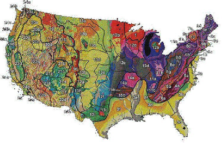
Figure 5. USACE (10) stream classification system.

PHYSIOGRAPHIC REGIONS

The United States can be divided into eight major physiographic regions based on geologic and geomorphologic characteristics. The major regions can be further subdivided into subregions, for a total of 25 physiographic regions. The boundaries of these regions are not strictly defined. Rather, the regions are approximately mapped to provide a description of major physiographic changes across the country. Figure 6 shows these regions based on a map created by Fenneman and Johnson. (62) The regions and subregions are:

• Region 1—Laurentian Highlands, including Superior Uplands.
• Regions 2–3—Atlantic Plain, including Coastal Plain and Continental Shelf.
• Regions 4–10—Appalachian Highlands, including Piedmont, Blue Ridge, Valley and Ridge, St. Lawrence, Appalachian Plateau, New England, Adirondack.
• Regions 11–13—Interior Plains, including Interior Low Plateau, Great Plains, Central Lowlands.
• Regions 14–15—Interior Highlands, including Ozark Plateaus, Ouachita Province.
• Regions 16–19—Rocky Mountain System, including southern Rocky Mountains, Wyoming basin, middle Rocky Mountains, northern Rocky Mountains.
• Regions 20–22—Intermontane Plateaus, including Columbia Plateau, Colorado Plateau, Basin and Range.
• Regions 23–25—Pacific Mountain System, including Cascade-Sierra Mountains, Pacific border, lower California.

Physiographic regions provide natural divisions by which to investigate stream processes and erosion issues broadly. Thornbury defined a physiographic unit as an area of land with similar or uniform topographic characteristics, including altitude, relief, and type of landforms, that are distinctly different from other physiographic units. (63) Dietz suggested that the erosion and sedimentation processes and the rates of those processes also define the topography and landforms. (64) Several publications describe the landforms and underlying geologic structure of each of the physiographic regions listed above. (63, 65, 66) The landforms result from the combination of the underlying geologic structure and the erosion processes on the surface. Thus, gross characteristics of the streams can be summarized for each of the physiographic Provinces. Within each of these Provinces, however, there is a range of stream types due to variability in valley slope, sediment supply, and water discharge. In addition, changes to the stream channels through engineering of channels (straightening, clearing, widening, dredging) and removal of riparian vegetation also have tremendous impacts on the form that the channel will take.

A number of studies supply evidence of the link between stream channel characteristics and physiographic region. Based on field observations and a detailed literature review, Graf characterized the physiographic Provinces and the stream types in each. (67) The recent activities in stream restoration have motivated a number of studies that attempt to characterize the morphologic characteristics of stream channels within a specific physiographic region. Most of these studies are focused on developing so-called regional equations that provide stream width and depth as a function of drainage area and/or bankfull discharge. These equations typically are developed within specific physiographic Provinces, thus providing additional evidence of common stream channel characteristics as a function of physiography. When comparing the regional equations with other sites, it should be kept in mind that the data for the equations are almost always collected at stream gages, which means that the site is likely to be stable. Thus, a comparison of widths and depths obtained from these equations with those measured at other sites may indicate relative stability of the observed site. These studies and others are summarized below for streams in selected regions to illustrate the variation in streams from one region to another.

Figure 6. Physiographic map of the United States (after reference 66).

Appalachian Highlands. Streams in this region are generally meandering and perennial; however, the pattern is greatly influenced by slope, geology, and bed materials. (68) In the higher elevations, the geology is generally (although with exceptions) more resistant material. Hack showed that slopes in the Shenandoah Valley are much steeper (about seven times steeper) than those in the Martinsburg, shale areas, while streams in the carbonate rock areas had slopes in between those of the Shenandoah Valley and Martinsburg, shale areas. (69) However, Hack also showed that the slopes of channels across the Appalachian region could be predicted by 18(d/A_D)^0.6(70), where A_D is the drainage area d is the median size of the bed material. Channel pattern in this region is also controlled by bedrock. The bedrock exposures and rough terrain tends to create waterfalls and fast-moving streams across the region. (71) Regional equation parameters, developed by the U.S. Geological Survey for the Appalachian Plateau of New York, are given in table 5. (72) The equations resulted in a width-to-depth ratio of 16.5A_D^0.09, which can be approximated as 16.5, since the exponent of 0.09 is quite small and has little effect on the width-to-depth ratio. Piedmont streams are moderately sloped, controlled by bedrock outcroppings. (71) Bed material is primarily sand and gravel. (73) A number of studies have determined the hydraulic geometry of Piedmont streams. The resulting regional equation parameters are given in table 4. Variation within the resulting width-to-depth ratios are significant, ranging from about 5.04 to 12.53. The range can be attributed to variability in levels of urbanization, land use, location within the Piedmont, and differences in observer identification of bankfull elevations.

Coastal Plain. Streams are perennial and primarily meandering with limited reaches of braiding where channel slopes are higher and sediment loads are greater. (74) Oxbow lakes, back-swamps, and natural levees are common. Engineered dams and levees are also common to control flooding. Coastal Plain stream bottoms consist of more easily erodible material than the neighboring Appalachian Highlands. (71) Stream slopes are primarily gentle with bed material consisting of sand to fine gravel. Studies have been conducted in several eastern States to determine the hydraulic geometry of streams in the Coastal Plain region. Sweet and Geratz developed the set of regional equation parameters for North Carolina's Coastal Plain, given in table 4. (75) Prestegaard found slightly different equations for width and depth, also given in table 4. (73) She determined average bed materials to be in the sand and gravel ranges with an average median sediment size of 8 millimeters (mm). She also found that, in general, Coastal Plain streams were deeper and narrower than Piedmont streams. This can be seen by comparing the width-to-depth ratios for each region.

Great Plains and Central Lowlands. Streams in the Great Plains and Central Lowlands can be ephemeral, intermittent, or perennial. The Great Plains represent a depositional environment, deriving sediment from the mountains to the west. Deposited sediment is then reworked and moved through the channel system. (76) Channel morphology in the Midwestern United States has been affected by water development projects. Several well-known geomorphic studies in the Great Plains have related channel geometry and hydraulic geometry sediment characteristics and flow discharge. (80, 81) Both the Central Lowlands and the Great Plains, as well as portions of the Interior Lowlands, are covered with thick deposits of loess. (82) Simon and Rinaldi conducted reconnaissance studies at streams throughout the Midwest and determined that the combination of easily erodible soils and extensive human disturbance has produced thousands of miles of highly unstable streams. (82)

Rocky Mountains. Local variations in geological setting and tectonics have significant control over fluvial processes and, thus, stream morphology. (83) Coarse-grained sediment is transferred from the mountains to the surrounding basins. Channels in the mountains are relatively steep and carry a coarse sediment load. In the adjacent basins, channels have lower gradients and transport finer grained materials that are derived, in part, from the coarser upstream load.

Basin and Range . This Province is primarily arid to semiarid. Thus, rivers in the Basin and Range tend to be ephemeral or intermittent. Alluvial fans are common in the Basin and Range. They develop when sediment transported along steep, mountain channels deposits on shallower slopes at the base of the mountains. Streams in alluvial fans are typically highly unstable in terms of lateral position. One of the most outstanding characteristics of rivers in the Basin and Range is that drainage across most of the Province is internal. (84) Castro and Jackson developed regional equation parameters, given in table 4, for the upper Basin and Range based on measurements at 22 stream channels. (79)

Pacific Coastal (California). The Pacific Coastal region in California is characterized by a wide variety of drainage types that include arroyos and alluvial fans. (85) Streams in both of these stream types tend to be unstable both laterally and vertically. Human alterations of stream channels in this region are widespread and have changed the erosion and depositional patterns. Streams may be ephemeral, intermittent, or perennial. Castro and Jackson developed regional equation parameters for this region, given in table 4. (79)

Table 4. Regional equation parameters for selected physiographic regions in the United States.

Previous | Contents | Next