• Federal Highway Administration >
• Publications >
• Research Publications >
• Hydraulics Publications >
• 07026 >
• 04.Cfm >
• Bottomless Culvert Scour Study: Phase II Laboratory Report

Bottomless Culvert Scour Study: Phase II Laboratory Report

Chapter 4: Results

The results presented in this section reflect the experiments described in the “Experimental Approach” section. The first subsection shows how these experiments compared with theoretical predictions of scour at the inlet of bottomless culverts. The second subsection presents scour maps that illustrate the scour that occurred at the culvert outlet. And the third subsection shows how the experiments relate to different scour countermeasures.

CLEAR WATER SCOUR EXPERIMENTS

This subsection presents the result of using laboratory experiments to determine the actual form of equations 4 and 11–13.

Representative Velocity

This section focuses on the calibration of V_RM. The representative velocities in the vicinity of the upstream corners of culverts were measured during fixed-bed experiments as prescour conditions. The measured V_RM values were then compared to the V_RP values from the potential flow theory to derive a multiplier, C, in equation 4, as illustrated in figure 10.

Figure 10. Graph. Calibration of C in equation 4.

A linear regression of the results shows that V_RM for bottomless culvert applications is 1.28 times V_RP. Thus, equation 4 can now be rewritten as equation 22.

(22)

Spiral Flow Adjustment Factors

Experiments were used to determine the form of the 12 different expressions for k_s. Two examples are given.

The first example is the calibration and validation of k_s as a function of V_RA, V_CL, and the Froude number. In this combination, y₂ was calculated from equation 1 using the approach velocity, V_RA (equation 2), and Laursen’s critical velocity, V_CL (equation 5). Figure 11 shows the regression of k_s versus the Froude number in the approach as the independent variable for bottomless culverts with and without wingwalls.

Figure 11. Graph. Calibration of k_s as a function of V_RA, V_CL, and F₁.

Figure 12 is a plot of y_max that was calculated using the regression equation from figure 11 versus the measured y_max.

Figure 12. Graph. Validation of y_max using kS as a function of V_RA, V_CL, and F1.

The second example is the calibration and validation of k_s as a function of V_RM, V_CN, and the Q_blocked ratio. In this combination, y₂ was calculated from equation 1 using the approach velocity, V_RM (equation 22), and Neill’s critical velocity, V_CN (equations 7 and 8). Figure 13 shows the regression of k_s versus the Q_blocked ratio as the independent variable for bottomless culverts with and without wingwalls.

Figure 13. Graph. Calibration of k_s as a function of V_RM, V_CN, and Q_blocked.

Figure 14 is a plot of y_max that was calculated using the regression equation from figure 13 versus the measured y_max.

Figure 14. Graph. Validation of y_max using k_s as a function of V_RM, V_CN, and Q_blocked.

Similar calculations and plots were obtained for the other ten k_s combinations. Table 2 summarizes the scour equation for each scenario for unsubmerged bottomless culverts, and some calibration and validation statistics. The Froude numbers in the experiments did not cover the full range that is expected in the field, and the negative slopes presented in table 2 are probably not realistic. For this reason, we recommend changing the Froude number multiplier to zero for equations in table 2 with negative slopes.

Note: As discussed in the text, the Froude number multiplier should be changed to zero for equations with negative slopes.

Pressure Flow Adjustment Factors

Although future experiments eventually will expand the range of the submerged flow conditions presented here, this section shows preliminary results for scour in a submerged bottomless culvert. These preliminary experiments were also used to determine the form of the 12 different expressions for k_p that correspond to the 12 different k_s equations in the previous section. Recall also that y₀ in equation 1 for pressure flow is equal to the hydraulic grade line at the inlet (HGL_o in figure 8). Two examples, similar to the k_s section, are given.

The first example is the calibration and validation of k_p as a function of A_k when k_s is a function of V_RA, V_CL, and F₁ (equations 13 and 14). In this combination, y₂ was calculated from equation 1 using the approach velocity, V_RA (equation 2), and Laursen’s critical velocity, V_CL (equation 5). Figure 15 shows the regression of k_p versus A_k as the independent variable for bottomless culverts with wingwalls.

Figure 15. Graph. Calibration of k_p when k_s is a function of V_RA, V_CL, and F1.

Figure 16 is a plot of y_max that was calculated using the regression equation from figure 15 versus the measured y_max.

Figure 16. Graph. Validation of y_max using k_p when k_s is a function of V_RA, V_CL, and F1.

The second example is the calibration and validation of k_p as a function of A_k when k_s is a function of V_RM, V_CN, and Q_blocked (equations 13 and 14). In this combination, y₂ was calculated from equation 1 using the approach velocity, V_RM (equation 22), and Neill’s critical velocity, V_CN (equations 7 and 8). Figure 17 shows the regression of k_p versus A_k as the independent variable for bottomless culverts with wingwalls.

Figure 17. Graph. Calibration of k_p when k_s is a function of V_RM, V_CN, and Q_blocked.

Figure 18 is a plot of y_max that was calculated using the regression equation from figure 17 versus the measured y_max.

Figure 18. Graph. Validation of y_max using k_p when k_s is a function of V_RM, V_CN, and Q_blocked.

All of the k_p equations derived in the preceding discussion can be substituted into equation 13 to obtain equations for the maximum scour depth in a submerged bottomless culvert. Table 3 summarizes the scour equation for each scenario. The Froude numbers in the experiments did not cover the full range that is expected in the field, and the negative slopes presented in table 3 are probably not realistic. For this reason, we recommend changing the Froude number multiplier to zero for equations in table 3 with negative slopes.

Note: As discussed in the text, the Froude number multiplier should be changed to zero for equations with negative slopes.

OUTLET SCOUR EXPERIMENTS

The bottomless culvert outlet scour experiments were completed in accordance with the test matrix (table 1). Specifically, the following results are presented and discussed:

• Fixed-bed prescour conditions, including velocity distributions analyzed using particle image velocimetry (PIV), for rectangular culverts with 45-degree wingwalls.

• Submerged entrance conditions for both fixed and movable bed conditions.

• Effects of various inlet and outlet wingwall configurations on resulting scour patterns (including location, lateral extent, and maximum depth of scour).

• Preliminary test of pile dissipator design to reduce outlet scour.

• Effectiveness of MDSHA Standard Plan to reduce scour.

• Revised stability coefficients and regression equations for sizing and placing riprap at entrances to bottomless culverts (originally presented in Phase I of this study) (discussed in a separate section).

• Performance of Rosgen-type cross vanes near bottomless culvert entrances, in the approach flow, as countermeasures to reduce culvert scour and channel instability (discussed in a separate section).

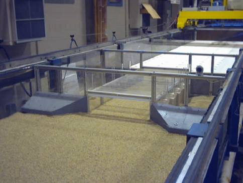
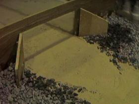
A sample of the resulting scour maps is given in appendix A. A table that summarizes the parameters for each experiment in appendix A is given in appendix B.

Flow Conditions

Fixed Bed

Fixed-bed tests were conducted to measure prescour conditions, which are the conditions best suited for the methodology proposed in Phase I to predict scour (figure 19). Detailed velocity distributions were measured at the culvert entrance using advanced techniques. A display of velocity distributions is provided in figure 20.

Figure 19. Photo. Outlet prior to scour test.

Figure 20. Image. Velocity distribution for unsubmerged culvert with 45-degree wingwalls at entrance.

From the fixed-bed experiments, it is clear that the vorticity increases as flow moves away from the culvert exit. The turbulent shear stress map in figure 21 shows very high shear stress at two locations a distance beyond the culvert outlet. These high shear stresses explain why scour holes are created in a moveable bed (figure 22). As shown in figure 23, adding wingwalls at the outlet reduces the shear stress, and thus reduces the outlet (downstream) scour hole depth (figure 24).

Figure 21. Image. Turbulent shear map for outlet with no wingwalls.

Figure 22. Image. Scour map for outlet with no wingwalls.

Figure 23. Image. Turbulent shear map for outlet with streamlined wingwalls.

Figure 24. Image. Scour map for outlet with streamlined wingwalls.

Movable Bed

Movable bed tests were conducted to measure scour conditions at the outlet for a variety of wingwall configurations (figure 25).

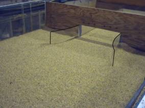
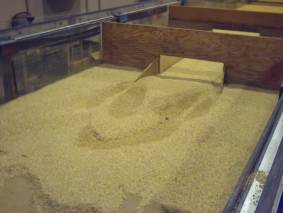
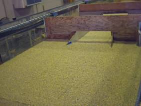
Figure 25. Photo. Outlet scour after test.

Submerged and Unsubmerged Conditions

Various inlet and outlet wingwall configurations were investigated under both submerged and unsubmerged flow conditions to determine the overall effects of the flow conditions on scour hole formation. The results show that submerged flow conditions induce greater inlet scour depths, while unsubmerged flow conditions induce greater outlet scour depths.

Wingwalls

Wingwalls have traditionally been constructed with highway culverts to increase flow capacity (for culverts operating in inlet control) and reduce the severity of erosion and scour of both the channel and adjacent banks at both the inlet and outlet. Various inlet and outlet wingwall configurations were investigated under both submerged and unsubmerged flow conditions to determine the overall effects of wall shape, length, and orientation on scour hole formation. The results from the experimental wingwall studies are covered in the following paragraphs. Maps for all of the resulting scour profiles can be found in appendix A.

Inlet Wingwalls

While the study focused on outlet scour, inlet wingwalls and their impacts on the scour at the inlet were also investigated. The experimental culvert setup was used to model a square culvert inlet with and without wingwalls for both submerged and unsubmerged flow conditions. Wingwalls were built with a 45-degree and an 8-degree flare.As demonstrated by the inlet experiments, upstream scour is deeper in submerged, pressure flow conditions. The results also show that 45-degree inlet wingwalls are effective at reducing inlet scour, whereas 8-degree inlet wingwalls are not effective. See table 4 and related figures 26 through 29.

Figure 26. Photo. 45-degree inlet wingwalls before scour.

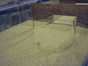
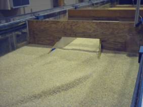
Figure 27. Photo. 45-degree inlet wingwalls after scour.

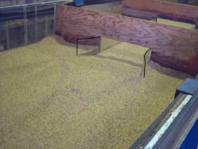
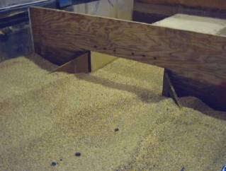
Figure 28. Photo. 8-degree inlet wingwalls before scour.

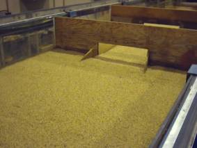
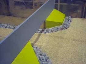
Figure 29. Photo. 8-degree inlet wingwalls after scour.

Outlet Wingwalls

As demonstrated by the outlet experiments, downstream scour is deeper in unsubmerged conditions (table 5). However, scour in unsubmerged conditions can be substantially reduced by the use of outlet wingwalls with a streamlined shape (compare figures referenced in table 5). Experimental results indicate that turbulence is reduced and “vortex shedding” caused by abrupt changes in pressure is almost eliminated by use of this shape. In other words, the streamlined wall eliminates flow separation and decreases turbulence.(10) Hence, with the streamlined bevel, vortices do not propagate downstream and the resulting turbulence is more evenly distributed—not concentrated in a single location. Conversely, the abrupt change in pressure that results from a square exit shape (as found in culverts without wingwalls at the outlet) induces vortex shedding and increased scour depths.

Figure 30. Photo. No wingwalls.

Figure 31. Photo. Truncated, circular wingwalls before scour.

Figure 32. Photo. Truncated, circular wingwalls after scour.

Figure 33. Photo. Elongated, streamlined wingwalls before scour.

Figure 34. Photo. Elongated, streamlined wingwalls after scour.

Figure 35. Photo. Short, streamlined bevel wingwalls after scour.

Figure 36. Photo. Wingwalls with 8-degree flare (rough joint) before scour.

Figure 37. Photo. Wingwalls with 8-degree flare (rough joint) after scour.

Figure 38. Photo. Wingwalls with 8-degree flare (smooth joint) before scour.

Figure 39. Photo. Wingwalls with 8-degree flare (smooth joint) after scour.

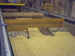
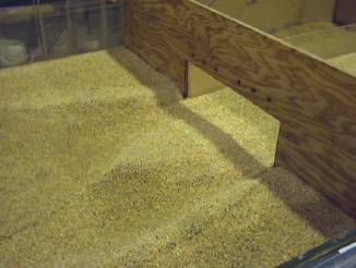
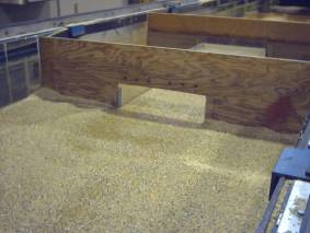
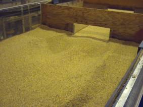
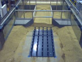
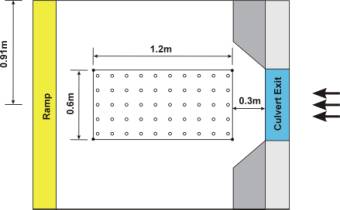
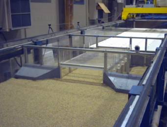
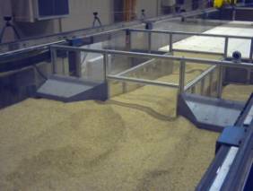
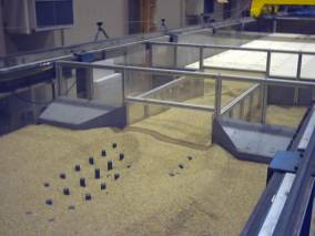
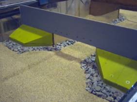
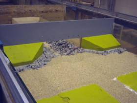
Figure 40. Photo. 45-degree wingwalls after scour.

Scour Countermeasures

Four scour countermeasures were evaluated other than wingwalls: riprap, cross vanes, pile dissipators at the outlet, and the MDSHA Standard Plan combination of countermeasures. The results of the riprap and cross vane analyses are presented later in this report.

Outlet Scour Control Using Pile Dissipators

Chang at MDSHA designed a series of group piles herein called pile dissipators (cylindrical pegs, 25 mm (0.975 inch) in diameter and 12 cm (4.68 inches) in height, mounted on a board) to reduce scour at the culvert outlet.(2) Table 6 lists the three tests used to evaluate this type of countermeasure, and the scour maps presented in appendix A that illustrate their effect. Figure 41 shows a photo of the pile dissipators used in the experiments, and figure 42 shows the position of the dissipators. Figure 43 shows the culvert prior to scour, while the last two photos show the resultant scour both without (figure 44) and with (figure 45) pile dissipators. The maximum scour depth without pile dissipators was 110 mm (4.29 inches), while the scour with dissipators ranged from 84 to 91 mm (3.28 to 3.55 inches). In other words, the pile dissipators decreased the scour depth by 17 to 26 percent.

Figure 41. Photo. Pile dissipators.

Figure 42. Diagram. Plan view of pile dissipators.

Figure 43. Photo. Culvert outlet prior to pile dissipator test.

Figure 44. Photo. Outlet scour area without protective pile dissipators.

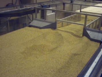
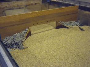
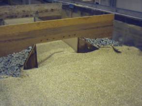
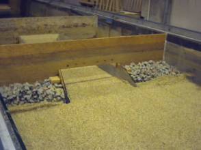
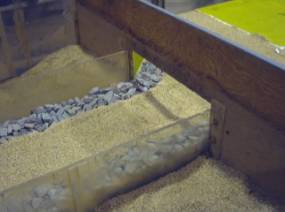
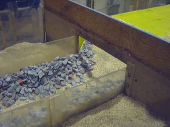
Figure 45. Photo. Outlet scour area with protective pile dissipators.

Scour Control Using MDSHA Standard Plan Methods

The MDSHA Standard Plan was tested as a scour countermeasure design. This design employs wingwalls at the inlet and outlet of the culvert and lines the wingwalls and the inside walls of the culvert with riprap (D₅₀ equals 25 mm (0.975 inches); see figures 46 and 47). The plan was tested under submerged conditions with 45-degree inlet wingwalls and both 45-degree and streamlined beveled outlet wingwalls. Figures 48 to 50 show the tests prior to scour with the riprap positioned along the corners of the culvert. The plan was tested with a flow depth of 23 cm (8.97 inches) and a velocity of 13 cm/s (5.07 inches/s). When the plan was tested, the riprap moved and fell into the scour holes, after which the riprap stabilized (figures 51 and 52). Table 7 shows the results. Since these results are still preliminary, this report does not make any recommendations about sizing or placing riprap for this design.

Figure 46. Diagram. Countermeasure installation for MDSHA Standard Plan (top view).

Figure 47. Diagram. Countermeasure installation for MDSHA Standard Plan (Section A-A from figure 46).

Figure 48. Photo. Culvert inlet before Standard Plan test.

Figure 49. Photo. Culvert barrel before Standard Plan test.

Figure 50. Photo. Culvert outlet before Standard Plan test.

Figure 51. Photo. Shifted riprap in culvert inlet after Standard Plan test.

Figure 52. Photo. Shifted riprap in culvert barrel after Standard Plan test.

RIPRAP STABILITY DESIGN COEFFICIENTS

The data collected were the local bed velocity (V_LB) and the average contraction velocity (V_AC), the ratio of which is plotted versus the Froude number in the contraction zone in figure 53.

Figure 53. Graph. Calibrated function for K_VM.

Figure 53 reveals that the equation for K_VM takes the form of equation 23.

(23)

Data collected for different riprap sizes (for which V_eff was calculated using equation 19) by measuring the local velocity prior to movement were used to calibrate K_RIP, which is plotted versus the Froude Number at the contraction in figure 54.

Figure 54. Graph. Calibration function for K_RIP.

The fitted relationship in figure 54 reveals that the equation for K_RIP takes the form of equation 24.

(24)

Rewriting equation 17 by inserting equations 18 and 19 in terms of D₅₀ produces equation 25.

(25)

Substituting equations 23 and 24, dividing both sides by y_o, and collecting similar terms yields equation 26.

(26)

Thus, the final dimensionless equation calculating D₅₀ from y_o and F_o is equation 27.

(27)

To validate the results, V_AC measurements and Froude number measurements were used to calculate the design D₅₀ using equation 27. Figure 55 shows that the calculated D₅₀ matches the D₅₀ of the riprap used in the experiments very well.

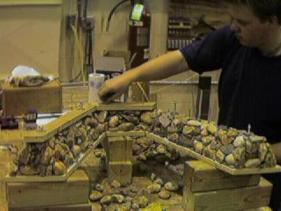
Figure 55. Graph. Validation of D₅₀ for riprap sizing.

USE OF CROSS VANES FOR INLET SCOUR CONTROL

Rosgen-type cross vanes, used near the modeled culvert entrance in the approach flow, were tested as a countermeasure for mitigation of inlet culvert scour and channel instability. The original intent of this set of experiments was to optimize cross vane geometry and location to minimize the amount of inlet scour. After determining that the cross vanes promoted more scour, the listed cross vane experiments were replaced with experiments using streamlined wingwalls at the exit. Figures 56 and 57 show the configuration and dimensions of the cross vanes, and figure 58 shows the fabrication of the cross vane. Figure 59 shows a photo of the culvert and cross vane before the experiment was run.

Figure 56. Diagram. Culvert with a cross vane.

Figure 57. Diagram. Experimental arrangement of culvert with a cross vane.

Figure 58. Photo. Fabrication of the cross vane.

Figure 59. Photo. Cross vane installed at inlet of experimental culvert.

The cross vane contributed to, rather than diminished, the effect of scour at the inlet. The cross vane creates a spiral current on each side of the cross vane and excavates the corners, the opposite of its desired intent. The flow field was measured at the entrance with PIV and the results show the spiral current effect (figure 60). Figure 61 shows that scour is increased when the cross vane is added.

Figure 60. Image. PIV image of flow field at culvert entrance showing spiral current in corners.

Figure 61. Graph. Cross vane results.

Previous | Contents | Next