U.S. Department of Transportation
Federal Highway Administration
1200 New Jersey Avenue, SE
Washington, DC 20590
202-366-4000
Federal Highway Administration Research and Technology
Coordinating, Developing, and Delivering Highway Transportation Innovations
 |
| This report is an archived publication and may contain dated technical, contact, and link information |
|
Publication Number: FHWA-HRT-04-044 Date: February 2004 |
Previous | Table of Contents | Next
Pavement engineers have many design feature options when designing a PCC pavement. Feature choices such as the selection of base type, drainage type, load-transfer mechanism, slab thickness, and joint sealant type all influence both the cost and expected performance of the resulting pavement section. As pavement designers always strive to maximize performance while minimizing cost, an understanding of the cost and performance influence of each chosen feature is imperative during the design process.
The estimation of the overall cost associated with the selection of different design features is straightforward, as all design feature costs are cumulative. The estimation of overall performance is, however, more complex, as there are many performance interdependencies among design feature choices. For example, a design engineer may estimate that by itself, using a cement-treated base instead of a dense aggregate base may improve overall performance by an estimated 5 percent. In another separate case, the design engineer may estimate that using a tied PCC shoulder instead of an asphalt shoulder would result in a 15 percent increase in performance. However, in actuality, if both design features were made at the same time, an interdependency between these two design features may result in an overall increase in performance of 18 percent (i.e., they are not necessarily cumulative). This software tool utilizes a simplified methodology that allows pavement engineers and contractors to estimate the performance associated with different design feature interdependencies. The results from this software therefore, can be used to estimate the relative cost effectiveness of different combinations of design features.
The contents of this appendix are intended to:
The remainder of this section includes an introduction to the general capabilities and intended uses of the software, followed by an introduction to the software's user interface structure.
This software provides a tool for pavement designers and contractors who are interested in investigating the cost and performance trade-offs associated with the selection of different design features during the PCC pavement design process. With this tool, you may define different pavement sections (i.e., different unique combinations of design features) that can then be compared to determine the relative differences in cost and performance of each section. However, before using the software, it is important to understand that it is absolutely not intended as a "design" tool. Instead, it provides a "reasonableness" check regarding the "justification" or "questioning" of the addition of different design features.
Specifically, the following two types of analysis sessions may be conducted using the software:
1) Direct Comparison-A Direct Comparison analysis session is used to compare two defined pavement sections in order to assess expected differences in cost and performance. A byproduct of this analysis type is the benefit/cost (B/C) ratio associated with each section. In a comparison of two pavement sections, the section with the largest B/C ratio is the most cost effective section to construct. Another way to interpret these B/C ratios is that the larger the B/C ratio, the more performance that is achieved per dollar spent.
2) Sensitivity Analysis-A Sensitivity Analysis session is provided as a method of defining more complex analysis sessions. Specifically, the following two general types of sensitivity analyses may be defined in the software:
Both of these general sensitivity analysis types are discussed in more detail later in this appendix.
It is important to note that the outputs (i.e., estimated cost and performance) of this tool are only as good as the reliability of the numerous inputs collected in the user interface. For example, the importance of choosing a representative cost data set, performance data set, and category ranking set are critical to the validity of the results. Because the default data sets provided in the software were based on collected survey data from all over the United States, it is strongly suggested that the user define cost sets, performance sets, and category ranking factor sets that reflect local experiences and conditions.
The user is also reminded that because this tool is built on simple mathematical concepts, the relative trends resulting from the analysis should be deemed more important than the actual values (i.e., the computed percent changes in cost and performance). Therefore, it is again emphasized that the output results from this tool are solely "estimates" of cost and performance associated with changing design features and, therefore, should be used with caution.
Before getting started using the software, it is important to understand the structure of the software's user interface and the data organization within the software.
The user interface is organized as a series of tabs. Brief descriptions of each of the tabs are provided below:
Defined pavement sections may be named and saved in the Pavement Section Master List. Those saved pavement sections will then be available to the user when defining an analysis session.
Also included within the Section Definition tab are controls that are used to define the inputs required to conduct a simplistic life-cycle cost analysis (LCCA) as part of a defined analysis session. When an analysis is conducted, these cost inputs combined with the expected changes in performance are used to compute simple expected life-cycle cost (LCC) streams associated with the different pavement sections being analyzed. The LCC approach is described as simplistic in that the cost stream values (annual maintenance, rehabilitation, and salvage value costs) can all be determined using simplified methods. However, because of its simplistic nature, the user of the software tool is warned that the results of the LCC analysis should be viewed with caution. While the cost trends may be realistic, the actual computed dollar values may or may not be accurate. If more accurate LCC analysis results are desired, it is recommended that a more rigorous LCC analysis be conducted using accepted methods.
More detailed descriptions of each of these tabs and their purpose, usage, and inputs are contained in the remaining sections of this appendix.
To effectively use this analysis software, you will need an IBM®-compatible industry-standard personal computer with the following minimum characteristics:
This is an auto-run CD-ROM (i.e., it should automatically launch when placed in your CD-ROM drive). If your current system is not set with "auto insert notification" enabled, you will have to run the SETUP.EXE in the root drive of the CD-ROM. Starting this .exe will launch the install program and/or the contents CD-ROM. Follow the on-screen instructions to complete the installation process. Upon completion, to start the software, select the "PCC Design Feature Comparison Tool" shortcut in your "Programs" list (under "All Programs" in Windows XP) under the "Start" menu.
As mentioned previously, this software uses a tabbed structure as the basis of its user interface (see figure 2). When you first open the program, a blank database is opened (i.e., no user-defined pavement sections, cost sets, performance sets, etc.) with the Introduction tab showing. The interactive flow chart on the left of this tab is included as a method of introducing the analysis process and its associated user interface components. To learn more about a particular step of the approach, place your cursor over one of the boxes in the flow chart. The remainder of this section introduces you to the menu and toolbar items that are visible as part of the software's interface. Each of the other tabs making up the interface is described in other sections of this appendix.
The menu bar includes three items: File, Edit, and Help. To display the available commands under a specific menu heading, click on the heading of your choice. You may then click on any of the commands shown in the associated drop-down list.
The File menu, shown in figure 3, contains eight standard windows commands, each of which is described briefly below.
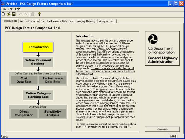
Figure 2. Software main window with the Introduction tab displayed.
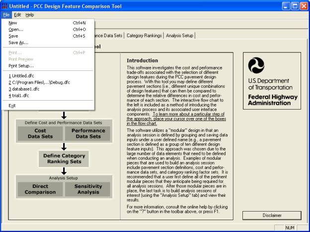
Figure 3. Contents of the File menu.
In addition to the standard windows commands, a list of the last four viewed databases (if available) will also appear in this file menu. To open a recently viewed database, simply select the name from the list.
The edit menu contains the following three commands:
The help menu contains the following three commands:
The toolbar buttons provide quick access to many of the commands housed in the software menus. Brief descriptions of each of the visible toolbar buttons are provided below. To activate a toolbar button, simply click on it.
![]() New-Creates a new database.
New-Creates a new database.
![]() Open-Opens an existing database.
Open-Opens an existing database.
![]() Save-Saves the current database.
Save-Saves the current database.
![]() Undo-Undoes the last software action completed by the user.
Undo-Undoes the last software action completed by the user.
![]() Redo-Restores any previously undone software actions in the reverse order that they were originally undone.
Redo-Restores any previously undone software actions in the reverse order that they were originally undone.
![]() Print-Activates the pop-up Print dialog box in preparation for printing information associated with the selected data module on the current tab.
Print-Activates the pop-up Print dialog box in preparation for printing information associated with the selected data module on the current tab.
![]() Help-Opens the Help File and displays help text that is associated with the user's current location in the software's interface.
Help-Opens the Help File and displays help text that is associated with the user's current location in the software's interface.
As mentioned previously, the software provides the user with a tool for investigating the cost and performance implications of changing different design features in a PCC pavement. Specifically, the software allows the user to change design features organized into the following 10 categories:
A summary of all available feature values associated with each of these design categories is summarized in table 20.
A pavement section is defined as a unique combination of specific feature values chosen from these 10 different design feature categories. That is, defining a section requires that the user select one of the provided feature choices (see table 20) for each of the different design categories. The remainder of this section starts by introducing the concept of the Standard pavement section. This is followed by a more detailed discussion of the individual controls on the Section Definition tab, and how they are used to define and save different pavement sections.
The cost and performance impacts of changing design features are all measured relative to a Standard pavement section. Specifically, the Standard section is defined as that pavement section with the specific design features summarized in table 21.
The Standard pavement section was used as the basis for the survey process as contractors and agencies were asked to estimate percent changes in cost and performance resulting from changing design features from the Standard pavement section. Specifically, survey respondents were asked to make subjective estimates of cost and performance changes resulting from changing one design feature at a time in the Standard pavement section. It is important to understand the detailed meaning of the Standard pavement section as it is referenced many times in the remaining chapters of this appendix.
The Section Definition tab provides controls that are used to define different pavement sections. As illustrated in figure 4, the left side of the tab contains the Pavement Section Master List while the right portion of the tab contains two secondary tabs titled Variables and Life-Cycle Costs. Each of these areas of the Section Definition tab is discussed separately below.
Design Category |
Design Feature Choices |
|---|---|
Subgrade |
|
Base/Subbase |
|
Drainage |
|
Thickness/Slab Size |
|
Cross Section |
|
Joints/Load Transfer |
|
Joint Sealing |
|
Shoulders |
|
Strength/Materials |
|
Smoothness/Ride |
|
Key: STD = Standard.
Design Category |
Design Features |
|---|---|
Subgrade |
Untreated prepared subgrade |
Base/Subbase |
150-mm (6-in) dense-graded aggregate base |
Drainage |
No drainage layers, no underdrains |
Thickness/Slab Size |
250-mm (10-in) JPCP with 4.6-m (15-ft) joint spacing |
Cross Section |
250-mm (10-in) uniform thickness |
Joints/Load Transfer |
32-mm (1.25-in) epoxy-coated dowels, 4.6-m (15-ft) perpendicular joints |
Joint Sealing |
Hot-poured rubberized asphalt with widening cut (4.6-m joint spacing) |
Shoulders |
150-mm (6-in) HMA over 250-mm (10-in) dense graded aggregate base |
Strength/Materials |
4.5-MPa (650 psi) flexural |
Initial Smoothness |
110 to 142 mm/km (7 to 9 in/mi) (measured with a 5-mm [(0.2-in]) blanking band) |
Note: Average daily traffic (ADT) is 20,000 vehicles per day in each direction with 15% trucks. This is approximately 700,000 to 800,000 ESALs per year in the design lane. Assume no growth in annual ESALs during the life of the pavement. |
|
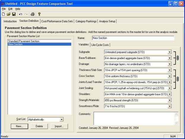
Figure 4. Section Definition tab with the Variables secondary tab displayed.
The Pavement Section Master List stores a complete list of the unique pavement sections defined within the current database. That is, the master list will always include the Standard Pavement Section and any user-defined pavement sections. You may sort this list alphabetically, by section creation date, or by section revision date by selecting the appropriate choice from the Sort List list box. This area also contains three buttons (New, Delete, and Import) that allow you to manage the contents of the master list. Specifically, the buttons perform the following functions:
![]() Creates and adds a new pavement section to the master list. Upon clicking this button, you will be prompted to enter a name for the new pavement section being created. Upon entering a unique section name, the new section name will be added to the master list. (Note that the new section will have the same design feature properties as the pavement section that was selected in the master list when the New button was clicked.)
Creates and adds a new pavement section to the master list. Upon clicking this button, you will be prompted to enter a name for the new pavement section being created. Upon entering a unique section name, the new section name will be added to the master list. (Note that the new section will have the same design feature properties as the pavement section that was selected in the master list when the New button was clicked.)
![]() Deletes the pavement section that is currently selected in the master list. Note that the Standard Pavement Section pavement section cannot be deleted from the list.
Deletes the pavement section that is currently selected in the master list. Note that the Standard Pavement Section pavement section cannot be deleted from the list.
![]() Imports a previously defined pavement section from another .dfc file. Upon clicking the Import button, use the controls of the pop-up Windows Explorer dialog box to locate the .dfc file from which you wish to import a pavement section. After selecting a .dfc file, click the Open button to bring up the Import dialog box (see figure 5). Select from the list the sections you wish to import and click OK. Those selected sections will be added to the master list.
Imports a previously defined pavement section from another .dfc file. Upon clicking the Import button, use the controls of the pop-up Windows Explorer dialog box to locate the .dfc file from which you wish to import a pavement section. After selecting a .dfc file, click the Open button to bring up the Import dialog box (see figure 5). Select from the list the sections you wish to import and click OK. Those selected sections will be added to the master list.
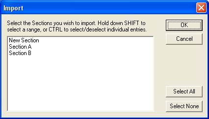
Figure 5. Example of the Import pop-up dialog box.
The controls of the Variables secondary tab (see figure 4) are used to select the specific design features associated with a given pavement section. To edit the feature details of a given section, you must first select the pavement section of interest from the Pavement Section Master List. To define the specifics of the selected section, choose a desired design feature from each of the list boxes associated with the 10 different design feature categories. You will notice that the last three items in each design category list box are user-definable custom names. Changes to these custom names may only be made when defining cost or performance data sets under the Cost/Performance Data Sets tab.
It must be noted that some design feature categories are inherently dependent on the settings of other categories (i.e., they are linked). Specifically, dependencies exist between the design categories of 1) subgrade, base/subbase, and drainage, and 2) thickness/slab size, cross section, joints/load transfer, and joint sealant. Each of these dependency groups is indicated in the user interface by the brackets and the associated ![]() (link) symbol (note: clicking on the
(link) symbol (note: clicking on the ![]() symbol in the user interface will open a pop-up dialog with a brief explanation of its meaning). The purpose of the link symbol is to alert the user that changing one of the design categories within a dependent set may automatically modify the settings of one or more of the other linked categories.
symbol in the user interface will open a pop-up dialog with a brief explanation of its meaning). The purpose of the link symbol is to alert the user that changing one of the design categories within a dependent set may automatically modify the settings of one or more of the other linked categories.
An example of a dependency within the first group of design feature categories is observed if you choose 300-mm (12-in) lime treated subgrade as your subgrade. When this subgrade selection is made, the base/subbase value will automatically be set to [(No base; placed directly on 300-mm (12-inch) stabilized subgrade]) and the drainage value will automatically be set to [(No drainage layers; 300-mm (12-inch) Lime Treated Subgrade]). These dependencies reflect the limited design feature choices that were allowed in the survey. All of the specific design feature dependencies between subgrade, base/subbase, and drainage are summarized in table 22.
An example of a dependency in the second set of linked fields is observed when the thickness/slab size is set to 250-mm (10-inch) JRCP with 9.1-m (30-ft) joint spacing (32-mm [(1.25-inch]) epoxy-coated dowels, 150-mm [(6-inch]) by 300-mm [(12-in]inch) mesh). When the JRCP pavement type is chosen, the joint/load transfer field is automatically set to [(Defined under Thickness/Slab Size]). In addition, the Joint Sealing field is set to the first custom joint-sealing value (e.g., Custom 1) as all of the default values in the joint sealing list are specific to a 4.6-m (15-ft) joint spacing. Table 23 summarizes all of the specific design feature dependencies between thickness/slab size, cross section, joints/load transfer, and joint sealant.
The bottom of the Variables secondary tab provides more general section-related feedback to the user. Use the Comments box to enter any general information you wish to save as part of the section definition. Also, note that for your convenience, the section definition creation and revision dates are included to indicate when the section definition was first and last saved in the Pavement Section Master List.
Design Feature Category |
Controlling Design Feature Selection |
Explanation of Resulting Dependencies |
|---|---|---|
Subgrade |
IF 300-mm (12-in) lime treated subgrade THEN |
|
IF subgrade equals anything but 300-mm (12-in) lime treated subgrade THEN |
No restrictions on base/subbase or drainage |
|
Base/Subbase |
IF 150-mm (6-in) dense-graded aggregate base (STD) THEN |
|
IF base type equals anything but 150-mm (6-in) dense-graded aggregate base (STD) THEN |
|
|
Drainage |
IF No drainage layers, no underdrains (STD) THEN |
No restrictions on subgrade or base/subbase. |
IF any drainage option (including custom drainage) is selected other than No drainage layers, no underdrains (STD) THEN |
|
Key: STD = Standard.
Design Feature Category |
Controlling Design Feature Selection |
Explanation of Resulting Dependencies |
Thickness/Slab Size |
IF 250-mm (10-in) JPCP with 4.6-m (15-ft) joint spacing (STD) THEN |
|
|---|---|---|
IF 200-mm (8-in) JPCP with 3.7-m (12-ft) joint spacing THEN |
Cross section, joints/load transfer, and joint sealing are limited to the Custom values due to a lack of 200-mm- (8-in-) related inputs. |
|
IF 300-mm (12-in) JPCP with 5.5-m (18-ft) joint spacing (38-mm [(1.5-in]) epoxy-coated dowels) THEN |
|
|
IF 250-mm (10-in) JRCP with 9.1-m (30-ft) joint spacing (32-mm [(1.25-in]) epoxy-coated dowels, 150-mm [(6-in]) by 300-mm [(12-in]) mesh) THEN |
|
|
IF 240-mm (9.5-in) CRCP (19-mm [(0.75-in]) epoxy-coated deformed bars, 200-mm [(8-in]) o.c. [(longitudinal]), 900-mm [(36-in]) o.c. [(transverse])) OR 240-mm (9.5-in) CRCP (19-mm [(0.75-in]) noncoated deformed bars, 200-mm [(8-in]) o.c. [(longitudinal]), 900-mm [(36-in]) o.c. [(transverse])) THEN |
|
|
Cross Section |
IF any of the non-custom pavement cross section choices are selected THEN |
|
IF a Custom pavement cross section choice is selected THEN |
No limitations on thickness/slab size, joints/load transfer, or joint sealing. |
|
Joints/Load Transfer |
IF any of the non-custom joints/load transfer choices are selected THEN |
|
IF a Custom joints/load transfer choice is selected THEN |
No limitations on thickness/slab size, cross section, or joint sealing. |
|
Joint Sealing |
IF any of the non-custom joint sealing options are selected THEN |
|
IF any of the Custom joint sealing options are selected THEN |
No limitations on thickness/slab size, cross section, or joints/load transfer. |
Key: STD = Standard; o.c. = on center.
Because design feature changes alter the expected performance (estimated service life) of a given pavement section, the associated LCC stream is also affected. To compute a LCC stream for a given pavement section, you need to know expected pavement service life as well as detailed expected cost information (i.e., cost types and amounts). Whereas the selected category ranking set is used to determine expected overall performance for a pavement section, the cost details needed for the simplistic LCCA are defined under the Life-Cycle Costs secondary tab (shown in figure 6).
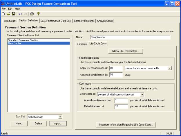
Figure 6. Section Definition tab with the Life-Cycle Costs secondary tab displayed.
The LCCA conducted within this software is described as simplistic in that the cost stream values (annual maintenance, rehabilitation, and salvage value costs) can all be determined using simplified methods. Because of its simplistic nature, the user of the software tool is warned that the results of the LCCA should be viewed with caution. While the cost trends may be realistic, the actual computed dollar values may or may not be accurate. If more accurate LCCA results are desired, it is recommended that a more rigorous LCCA be conducted using established methods.
Within the software's user interface, cost-related parameters are referred to as either global or pavement section-specific. The details of each of these LCCA parameter types are described separately in the following sections.
Those cost-related inputs that do not change between defined analysis sessions are referred to as global LCC parameters. Within the user interface, access to these global inputs is obtained by either clicking on the ![]() button or by selecting Global LCC Parameters from the Edit menu. Either action will cause the Global Life-Cycle Cost Parameters pop-up dialog box to appear (see figure 7).
button or by selecting Global LCC Parameters from the Edit menu. Either action will cause the Global Life-Cycle Cost Parameters pop-up dialog box to appear (see figure 7).
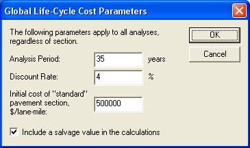
Figure 7. Global Life-Cycle Cost Parameters pop-up dialog box.
The remainder of this section contains detailed descriptions of each of the global cost-related inputs included on the Global Life-Cycle Cost Parameters pop-up dialog box.
Although it is not a user-definable global input, it is important to mention that the design life for the Standard pavement section is hard coded in the software as 20 years. This value is important because other pavement section expected lives are computed by multiplying this 20-year design life by the expected performance ratio computed by using the analysis methodology. For example, if a custom section were found to have an overall modified expected performance of +7.0 percent, the expected design life of the custom section is computed as 1.07 * 20 years = 21.4 years.
All annual maintenance and rehabilitation-related LCCA inputs are section-specific within the analysis approach. That is, all of these LCC inputs may be customized for each unique pavement section that is defined. The primary purpose of linking these cost inputs to a section is to accommodate the many cases where the inclusion of a design feature directly influences the future maintenance and rehabilitation costs associated with that section (e.g., including edge drains will result in the additional cost of cleaning the edge drains).
The remainder of this section contains detailed descriptions of each of section-specific LCC parameter inputs included on the Life-Cycle Costs secondary tab.
The primary outputs of this simplified LCCA are the individual computed costs defining the associated LCC stream, their computed total present worth value, and the associated equivalent uniform annual cost (EUAC).
The analysis approach allows the user to estimate the cost effectiveness of a given pavement section by computing total expected changes in cost and performance associated with the selection of different design features. These overall expected changes are computed as functions of user-defined cost and performance data sets that summarize the expected cost and performance impacts, respectively, associated with changing individual design features. A data set is defined as a summary of the relative percent changes in cost or performance associated with all possible design features available in each of the 10 design categories. The Cost/Performance Data Sets tab (shown in figure 8) is provided as a means of defining both types of data sets. Although each is similar in structure, the details of working with each data set type are discussed separately below.
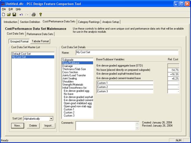
Figure 8. Cost/Performance Data Sets tab with the Grouped Format controls for the Cost Data Sets secondary tab visible.
The definition of cost or performance data sets requires a large number of input values to be defined for each. To facilitate the definition of these many data, the software allows the user to enter relative cost or performance data within one of two data-entry interface types termed Grouped or Tabular formats. Each of these interface types is introduced below.
The Grouped format (the default data-entry format) is divided into a Master List area and a Details area. The Cost Data Sets and Performance Data Sets master lists respectively store complete lists of the unique cost and performance data sets defined within the current database. You may sort these lists alphabetically, by section creation date, or by section revision date by selecting the appropriate choice from the associated Sort List list box. As with the Section Definition Master List, this area also contains New, Delete, and Import buttons that allow you to manage the contents of the master lists.
The Details area is used to specify the specific expected relative cost or performance values associated with choosing different design features. To edit the details of a given data set, start by selecting the data set from the corresponding master list. Next, select a design feature category from that provided list (note that the smoothness inputs are specific to different base types). When this selection is made, the specific design feature choices and associated input values for the given design feature category are displayed. Finally, use the provided input values to define the current data set. (Note: guidance on defining specific relative cost or performance values is provided below in the Defining Cost Data Sets and Defining Performance Data Sets sections, respectively).
In the Tabular format interface (displayed in figure 9), each data set in the master list is presented in a separate column in the table. Use the provided scroll bars to access the specific data set you wish to alter and make appropriate changes within the provided table. This area contains three buttons (Add Set, Delete Set, and Export Table) that perform the following functions:
![]() In this Tabular view, new data sets can be added to the master list using this button.
In this Tabular view, new data sets can be added to the master list using this button.
![]() Existing data sets may be removed from the master list by clicking on a cell in the column associated with the data set of interest, and then clicking this button. Note that the default cost and performance data sets can not be deleted.
Existing data sets may be removed from the master list by clicking on a cell in the column associated with the data set of interest, and then clicking this button. Note that the default cost and performance data sets can not be deleted.
![]() The current summary table of cost or performance data sets may be exported to an external electronic file by clicking this button. Upon clicking the
The current summary table of cost or performance data sets may be exported to an external electronic file by clicking this button. Upon clicking the ![]() button, use the controls provided in the Save Table As dialog box to select a file name, type, and storage location.
button, use the controls provided in the Save Table As dialog box to select a file name, type, and storage location.
Cost data sets are collections of expected changes in total cost resulting from the change of one design feature at a time. The changes in cost are expressed as expected percent changes in relation to the default Standard pavement section (see table 21). This is an extremely important point as the impact of all feature changes must be referenced back to the Standard pavement section. Therefore, you must complete the following procedure to define a complete cost data set:
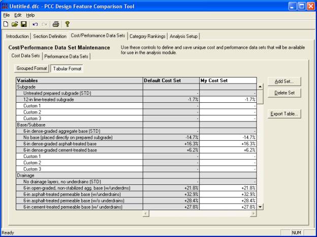
Figure 9. Cost/Performance Data Sets tab with the Tabular Format controls for the Cost Data Sets secondary tab visible.
This four-step process systematically defines a complete cost data set that covers all possible individual design feature changes from the standard pavement section. The following two examples illustrate the completion of steps 1, 2, and 3 for base/subbase and initial/smoothness, respectively.
Assume you are currently defining relative costs associated with the available base types in the base/subbase category. Recall that the Standard pavement section is defined with a base type of 150-mm (6-in) dense-graded aggregate base. The following paragraphs discuss the thinking a user should follow when trying to estimate cost changes associated with making base type changes.
The first base type that needs a relative cost value defined (i.e., the first base type after that used for the Standard section) is the choice of No base (placed directly on prepared subgrade). For this example, you would ask yourself, "If I remove the 150-mm (6-in) dense-graded aggregate base and build the Standard pavement section directly on the prepared subgrade, what percent change in original total construction cost (of the Standard section) would I expect to observe?" If you estimate that this base type substitution might save 14.7 percent in the total expected construction cost, then you would enter "-14.7" in the associated relative cost field. Note: This is the case for the example presented in figure 8.
Continuing the methodical investigation of base/subbase type, you would then define the case for the next base type in the list (i.e., 150-mm [(6-in]ch) dense-graded asphalt-treated base [(ATB])). For this case, you would ask yourself, "What percent change in original total construction cost would I expect to observe if I substitute a 150-mm (6-in) dense-graded asphalt-treated base in place of the Standard section's 150-mm (6-in) dense-graded aggregate base?" If, for example, you estimate that the Standard section would cost 16.3 percent more as a result of using an ATB, then you would enter "16.3" in the associated relative cost field (as shown in figure 8).
To complete this procedure, you must define an appropriate relative cost value for every base/subbase type (design feature value) included in the base/subbase list. Note: leaving a relative cost field blank is the same as setting it equal to "0." A relative cost value of "0" is appropriate for those cases where you can safely say that making that specific design feature change will not impact the overall cost of the Standard pavement section.
You will notice that three Custom fields (initially titled Custom 1, Custom 2, and Custom 3) are included in each design category. These are user-definable fields that are included to provide flexibility in the software by allowing the user to customize the software to match typically used design features. Figure 10 illustrates a case in which a user has defined a 200-mm (8-in) dense-graded aggregate base in the first custom field. For this case, the user has assumed that constructing the 200-mm (8-in) dense-graded aggregate base will cost 2.5 percent more than constructing the 150-mm (6-in) dense-graded aggregate base defined as part of the Standard pavement section. Note that the custom field names may only be changed within the Cost/Performance Data Sets tab (i.e., you cannot define custom field names under the Section Definition tab).
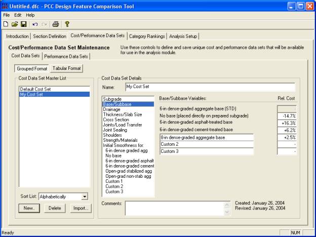
Figure 10. Example of using the provided custom design feature fields to reflect an agency's custom design features.
The definition of relative costs associated with different initial smoothness ranges is different from other design feature categories in that the relative costs are also dependent on different base types. Therefore, the first step in defining smoothness-related relative cost values is to select one of the base types listed under Initial Smoothness for: in the design feature category list. Figure 11 illustrates an example in which relative cost values were defined for the scenario in which a 150-mm (6-in) dense-graded asphalt-treated base was used in place of the Standard section's 150-mm (6-in) dense-graded aggregate base.
To accurately interpret the meaning of these smoothness-related relative cost values, you must keep their specific meaning in mind. The +3.3 percent value associated with the 110 to 142 mm/km (7 to 9 in/mi inches/mi) smoothness range (associated with a 5-mm [(0.2-in]ch) blanking band) may seem confusing at first as you might expect this value to be 0 percent since this 110 to 142 mm/km (7 to 9 in/miinches/mi) smoothness range is the smoothness range used to define the Standard pavement section. However, you must remember that for the different base types, the relative cost values associated with this Standard smoothness range (110 to 142 mm/km [(7 to 9 inches/mi)])
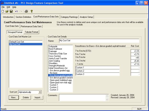
Figure 11. Example showing chosen relative cost values associated with a 150-mm (6-inch) dense-graded asphalt-treated base.
indicates of how much more or less smoothness-related preparation time is associated with the given base type. Specifically, for our example, the user indicated that achieving a target 110 to 142 mm/km (7 to 9 inches/mi) smoothness range is expected to cost 3.3 percent more if constructing on a 150-mm (6-inch) dense-graded asphalt-treated base than it would if constructing on a 150-mm (6-inch) dense-graded aggregate base.
For the remainder of the initial smoothness range inputs, the user must remain cognizant of the fact that the entered costs must only reflect the additional or reduced costs associated with achieving the target smoothness value. That is, although smoothness-related costs are entered for a series of different base types, the changes in the cost of the base layer are not to be included in these smoothness-related cost numbers. Costs associated with changing base types are those values entered under the base type category.
In the example displayed in figure 11, the user has decided that achieving 79 to 110 mm/km (5 to 7 inches/mi) on a 150-mm (6-inch) dense-graded asphalt-treated base would cost 3.7 percent more than achieving 110 to 142 mm/km (7 to 9 inches/mi) on a 150-mm (6-inch) dense-graded aggregate base (i.e., the Standard base type and initial smoothness values). Another way to look at this +3.7 percent number is to only look at the numbers within a given base type. Because we already have an indication of the smoothness-related cost strictly associated with the base type difference (i.e., +3.3 percent), it is the difference between the ATB-related relative cost values that give an indication of the costs associated with additional work required to achieve a smoother pavement for a given base type. In our example, the user has indicated that (assuming an ATB) it will cost +0.4 percent more to increase smoothness from 110 to 142 mm/km (7 to 9 in/miinches/mi) to 79 to 110 mm/km (5 to 7 in/miinches/mi) (i.e., +3.7 percent - 3.3 percent = +0.4 percent); +0.7 percent more to increase smoothness from 110 to 142 mm/km (7 to 9 in/miinches/mi) to 47 to 79 mm/km (3 to 5 in/miinches/mi) (i.e., +4.0 percent - 3.7 percent = +0.7 percent); +2.1 percent more to increase smoothness from 110 to 142 mm/km (7 to 9 in/miinches/mi) to 16 to 47 mm/km (1 to 3 in/miinches/mi) (i.e., +5.4 percent - 3.3 percent = +2.1 percent); and +3.8 percent more to increase smoothness from 110 to 142 mm/km (7 to 9 in/miinches/mi) to < 16 mm/km (< 1 in/miinches/mi) (i.e., +7.1 percent - 3.3 percent = +3.8 percent). To complete the cost data set, values must be defined for all combinations of base type and initial smoothness range.
Performance data sets are presented in exactly the same structure as cost data sets. However, instead of storing a collection of relative cost data, performance data sets are collections of expected changes in total performance resulting from the change of one design feature at a time. As with the cost data sets, the changes in performance are expressed as expected percent changes in relation to the expected performance of the Standard pavement section. This is an extremely important point as the impact of all feature changes must be referenced back to the Standard pavement section. This concept is best explained by the following two examples. (Note: although only two examples are presented, the complete definition of a performance data set involves defining relative performance values for each design feature value within each of the 10 design feature categories.)
Using the same examples provided in the cost data sets discussion, let's assume you are currently defining relative performance values associated with the available base types in the base/subbase category. Recall that the standard section is defined with a base type of 150-mm (6-in) dense-graded aggregate base. The following paragraphs discuss the thinking a user should follow when trying to estimate performance changes associated with making base/subbase type changes.
The first base/subbase type that needs a relative performance value defined (i.e., the first base type after that used for the Standard section) is the choice of No base (placed directly on prepared subgrade) (see table 20). For this example, you would ask yourself, "If I remove the 150-mm (6-in) dense-graded aggregate base and build the Standard pavement section directly on the prepared subgrade, what percent change in pavement performance (pavement life) would I expect to observe?" Again, you are reminded that the baseline performance that should be used for comparison is the expected performance of the default Standard section. If you estimate that this base type substitution might result in a decrease in performance of 20.0 percent (i.e., the new section will carry 20.0 percent fewer ESALs than the Standard section), then you would enter "-20.0" in the associated relative performance field. Note: This specific example is the case for the example presented in figure 12.
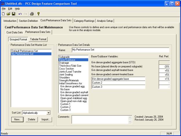
Figure 12. Example showing defined relative performance values associated with different base type choices.
The next base/subbase type in the list to be considered in the investigation is the 150-mm (6-inch) dense-graded asphalt-treated base. For this case, you would ask yourself, "What percent change in expected performance would I expect if I substituted the Standard section's 150-mm (6-inch) dense-graded aggregate base with a 150-mm (6-inch) dense-graded asphalt-treated base?" The user-defined numbers presented in figure 12 indicate that the user expected to increase the Standard section's allowable ESALs by 5.0 percent as a result of substituting base types.
As with the cost data sets, you must define an appropriate relative performance value for every base/subbase type (design feature value) included in the base/subbase list (including the custom fields). For completeness, this definition procedure must be completed for all 10 of the design feature categories. Note: Leaving a relative performance field blank is the same as setting it equal to "0." A relative performance value of "0" is appropriate for those cases where you can safely say that making that specific design feature change will not change (increase or decrease) the overall expected performance of the Standard pavement section.
Note: The user has the same access to the custom field names in both the Cost Data Sets and Performance Data Sets tabs. Therefore, a custom name defined when entering a cost data set will be reflected when defining performance data sets. Also note that custom field definitions are global in the sense that they are the same for all cost and performance data sets in the database (i.e., you cannot enter custom names that apply to specific cost or performance data sets).
The relative performance changes (increase or decrease in pavement life) associated with different pavement initial smoothness ranges can be viewed as an estimate of the effect of dynamic loading effects on the pavement. That is, many believe that rougher pavements cause dynamic movements in vehicles, resulting in dynamic loadings that cause an increased deterioration of the pavement, therefore decreasing service life. These changes in expected pavement life should be quantified in this portion of the user interface.
The definition of relative performance associated with different initial smoothness ranges is different from other design feature categories in that the relative performance is associated with combinations of base/subbase type and initial smoothness range. Although the expected performance changes associated with different initial smoothness ranges are not expected to be greatly influenced by the underlying base type, performance is still entered for different combinations of smoothness range and base/subbase type to maintain consistency with the cost data sets. You will note that in the default performance data set, the expected performance differences associated with different initial smoothness ranges are the same for all of the included base types.
The first step in defining smoothness-related relative cost values is to select one of the base types listed under Initial Smoothness for: in the Design Feature Category list. Figure 13 illustrates an example (in tabular format) in which relative performance values were defined for different initial smoothness ranges. To accurately interpret the meaning of these smoothness-related relative performance values, you must keep their specific meaning in mind. An investigation of the Default Performance Set finds a value of +2.0 percent associated with the 79 to 110 mm/km (5 to 7 in/miinches/mi) smoothness range (measured with a 5-mm [(0.2-in]ch) blanking band). This value indicates that a pavement constructed with an initial smoothness value in the 79 to 110 mm/km (5 to 7 in/miinches/mi) range (based on an 5-mm [(0.2-in]ch) blanking band) is expected to carry 2.0 percent more ESALs than the same pavement constructed with an initial smoothness value in the 110 to 142 mm/km (7 to 9 in/miinches/mi) range. That is, these expected changes in performance are solely due to the reduced initial smoothness value (i.e., most likely interpreted as the influence of initial smoothness on dynamic traffic loading-related damage). Therefore, when defining values associated with different combinations of initial smoothness and base/subbase type, be careful that you do not include the performance impact of changing the base/subbase type. The influence of base/subbase type on performance is represented under the base/subbase type design feature category inputs.
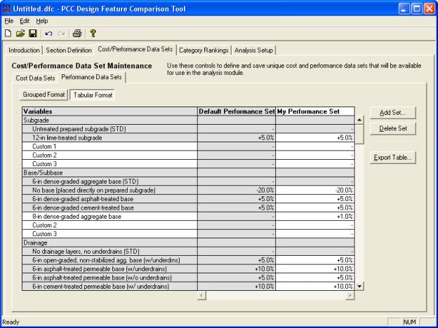
Figure 13. Example showing defined relative performance values associated with different initial smoothness choices.
As noted previously, determining the overall expected change in performance is not as simple as summing the expected performance changes associated with changing different design features individually. For example, if we assume that the removal of dowels will decrease the expected performance by 20.0 percent, but the addition of the CTB will increase performance by 5.0 percent, this does not necessarily mean that overall performance will be reduced by 15.0 percent. Therefore, as explained in chapter 3 of the report, the combined performance is estimated by making use of user-defined design feature category ranking factors.
As with the cost and performance data sets, the software allows you to define and save different category ranking sets. A category ranking set is defined as a unique combination of ranking factors (integers from 1 to 10) chosen for each of the 10 different design feature categories. No two design features were allowed to share the same ranking, so the result is essentially a "forced ranking" of the importance of each design feature category. The remainder of this section includes an introduction to the Category Rankings tab and guidance on defining your own ranking factor sets.
The Category Rankings tab (shown in figure 14) provides controls that are used to define and edit user defined category ranking sets. The tab is divided into two areas titled Category Rankings Master List and Category Ranking Set Details, each of which is discussed separately below.
The Category Ranking Set Master List stores a complete list of the all category ranking sets defined within the current database. In addition to the user-defined category ranking sets, this master list also contains the Default Rankings set (shown in table 24) that is based on a combination of average survey results and expert opinion. Note that the default ranking factor list in table 24 is presented in descending order or importance (i.e., the most important category is assigned a value of 10 while the least important category is assigned a 1).
As with the other master lists in the software, you may use the supplied Sort List list box to sort the Category Rankings Set Master List alphabetically, by ranking set creation date, or by ranking set revision date. This area also contains New, Delete, and Import buttons that allow you to manage the contents of the master lists by creating new, deleting existing, or importing existing defined ranking factor sets, respectively. Note, however, the Default Rankings set cannot be deleted or altered by the user.

Figure 14. Category Rankings tab.
| Design Category | Ranking Factor | |
|---|---|---|
Joints/Load Transfer |
10 |
Most Important |
Thickness/Slab Size |
9 |
|
Base/Subbase |
8 |
|
Drainage |
7 |
|
Strength/Materials |
6 |
|
Subgrade |
5 |
|
Initial Smoothness |
4 |
|
Joint Sealing |
3 |
|
Cross Section |
2 |
|
Shoulders |
1 |
Least Important |
The Category Ranking Set Details area is used to define and edit user-defined category ranking sets. To edit the relative weights assigned to each design feature category, click on the ranking factor set of interest in the Category Ranking Set Master List and then enter appropriate values in the provided Ranking Factors input boxes. Note that whenever a ranking factor value changed, the displayed ranking factor list is immediately resorted in descending order to reflect the change. When defining a ranking factor set, you must abide by the following three value-associated rules:
To assign meaningful design feature category ranking factors, it is first important to understand specifically how these values are used. The following section contains a discussion that provides the reader with a better understanding of how ranking factors are used in the performance computations, thereby helping you to select ranking factors that correspond with your assumptions of each design category's impact on performance.
One of the most difficult steps in the analysis approach is the assignment of category ranking factors that accurately reflect an agency's assessment of which design feature categories have the largest impact on overall performance. The use of defined ranking factors by the software is best explained with an illustrative example. Let's assume that we have an example (summarized in table 25) in which the subgrade, base/subbase, and drainage design features are changed simultaneously.
Design Feature Category |
Standard Section Feature |
Custom Section Feature |
Expected Relative Performance (%) |
Ranking Factor |
Normalized Impact Multiplier |
Modified Performance (%) |
|---|---|---|---|---|---|---|
Subgrade |
Untreated prepared subgrade |
300-mm (12-in) lime treated subgrade |
+5.0/ |
5 |
(5/8) = 0.625 |
+3.1 |
Base/ Subbase |
150-mm (6-in) dense-graded aggregate base |
150-mm (6-in) ATB |
+5.0 |
8 |
(8/8) = 1.00 |
+5.0 |
Drainage |
No drainage layers, no underdrains |
150-mm (6-in) ATPB with underdrains |
+10.0 |
7 |
(7/8) = 0.875 |
+8.8 |
TOTAL |
+16.9 |
In this example, the relative performance values of +5.0 percent, +5.0 percent, and +10.0 percent, respectively, were retrieved from the default performance data set. Next, we assume that the selected category ranking set contained factors of 5, 8, and 7 for the design categories of Subgrade, Base/Subbase, and Drainage, respectively. The associated ranking factors are then converted into normalized impact multipliers based on the largest observed ranking factor for only those design features changing from the Standard pavement section. For our example, the largest impact factor associated with the three changing feature categories is the "8" associated with Base/Subbase. Therefore, all three of the included impact factors are divided by "8" to compute normalized impact multipliers. These normalized impact multipliers are then multiplied by the associated expected relative performance values to give a modified performance value for each design category. The overall section performance is then determined as the sum of all modified performance values. For this example, the expected increase in performance is estimated to be 16.9 percent.
It is important to note that within this methodology, it is the relative differences between ranking factors rather than the actual ranking factor values that are important when determining overall modified performance. For example, one might think that the design feature assigned an impact factor of 10 is always going to be important when determining the overall pavement section performance. The previous example shows that this is not the case, as none of the three changing design feature categories had an impact factor of 10. Normalizing all individual ranking factors to the largest of the included factors ensures that the performance of the most important included design feature becomes the starting point of the modified performance computation. In the example, it is noted that if Base/Subbase were the only design feature category that was changing, then the total modified performance would be +5.0 percent. Therefore, the other design features deemed less important are, in a sense, used to adjust the +5.0 percent value associated with Base/Subbase. The normalized ranking multipliers give an indication of the relative impact of the adjustments.
When selecting category ranking factors, it is very important to assign factors that do not contradict the performance values observed within different design categories. That is, those design categories where the largest percent increases or decreases in performance are observed should most likely be the design categories with the largest category ranking factors. For example, assume that investigated Thickness/Slab Size choices result in individual performance changes from -40 to +50 percent, while different Joint Sealing choices result in a range of individual performance between -5 and + 5 percent. For this case, the category ranking factor assigned to Thickness/Slab Size should be significantly larger than that assigned to the Joint Sealing.
It is equally important to remember that the modified performance values resulting from the application of ranking factors are additive with the individual performance associated with the largest ranking factor is used as the starting point (e.g., the +5.0 percent was used as the starting point of the overall performance computation in the example illustrated table 25). This is because the category with the largest associated ranking factor is assumed to have the largest influence on overall performance. That is, in many cases, one should expect the overall performance to be close to the one individual performance value associated with the largest ranking factor as, by definition, it is the governing performance value. As mentioned previously, the ranking factors associated with other included design features are used to diminish those associated individual performance changes before adding them to the overall performance calculation. That is, all design feature categories that are not deemed to be the most important category (i.e., their ranking factors are less than the largest included ranking factor) are simply used to adjust the individual performance change associated with the largest ranking factor. It is the defined ranking factors that are used to determine the ranking factor ratios (normalized ranking multipliers) that determine the how much of each individual performance change is added to the overall performance value.
The final tab of the user interface is the Analysis Setup tab. Using the controls of this tab, the user may setup, define, and conduct two different types of analysis sessions (i.e., Direct Comparison and Sensitivity Analysis sessions). Also provided are controls that allow the user to customize the contents of an output report using an on-screen preview window. The remainder of this chapter includes an introduction to the Analysis Setup tab, brief explanations of the purpose of the Direct Comparison and Sensitivity Analysis session types, and detailed information on the methods and controls used to define both analysis session types.
The Analysis Setup tab (shown in figure 15) provides controls that are used to define and conduct two different types of analysis sessions: Direct Comparison sessions and Sensitivity Analysis sessions. Upon activating the tab, the user is first presented with two master lists representing these respective analysis types. (Note: When you are working with a new database, these master lists initially will be empty.)
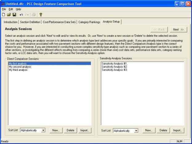
Figure 15. Example of the Analysis Setup tab.
Each master list stores a complete list of the all defined analysis sessions (by analysis type) defined within the current database. As with the other master lists in the software, you may use the respective Sort List boxes to sort each master list alphabetically, by creation date, or by revision date. This area also contains New and Delete buttons that allow you to manage the contents of the master lists by creating new or deleting existing analysis sessions, respectively.
The first step in defining an analysis session is to determine which analysis type best addresses your specific goals. If you are primarily interested in comparing the costs and performance associated with two pavement sections with different design features, then the Direct Comparison analysis type is the choice for you. However, if you are interested in conducting a more complex sensitivity-type analysis such as comparing one pavement section to a series of other sections, or investigating the different effects resulting from comparing a series (more than one) cost data sets, performance data sets, or category ranking factor sets, then you will want to choose the Sensitivity Analysis option. More specific discussions of both of these two analysis types are defined below.
The Direct Comparison analysis type is used to compare two defined pavement sections labeled Section A and Section B in the analytical tool) to assess the expected differences in cost and performance between the sections. By carefully defining different pavement sections, this analysis type is used to directly assess the cost and performance impact of changing one or more design features. Note that in a Direct Comparison analysis, the other data collection modules (the cost data set, performance data set, and category ranking set) are all held constant in the analysis.
The Sensitivity Analysis type is included for users who want to conduct more complex one- or two-dimensional sensitivity analysis investigations. These analysis sessions are defined by: 1) selecting one primary pavement section to be used as the basis for the investigation; 2) selecting one of five different analysis session types from a provided list (these are described below); and 3) selecting the specific parameters that define the scope of the analysis.
The following are the five specific types of sensitivity analyses from which the user may choose:
When you create a new (or edit an existing) Direct Comparison analysis session, the dialog box presented in figure 16 is displayed. The controls on this dialog box lead the user through a series of steps that will complete the setup of a Direct Comparison analysis session. After
the analysis session setup steps have been completed to your satisfaction, click the ![]() button to view the analysis results. Alternatively, click the
button to view the analysis results. Alternatively, click the ![]() button to return to the analysis session master lists. Each specific control on this page is described in detail in this section.
button to return to the analysis session master lists. Each specific control on this page is described in detail in this section.
To change the name of the current Direct Comparison analysis session, enter the new name in the Name input box. Note: The name displayed in the input box is the name that will be displayed in the Direct Comparison Sessions master list.
The first step in defining the Direct Comparison analysis session is the selection of the first pavement section to be compared (Section A). To define Section A, select a named pavement section from the list box within the Step 1: Select Section A area (note: The named pavement sections contained in this list box are those pavement sections stored in the Pavement Section Master List.) When you select a section from the list, the design category values associated with
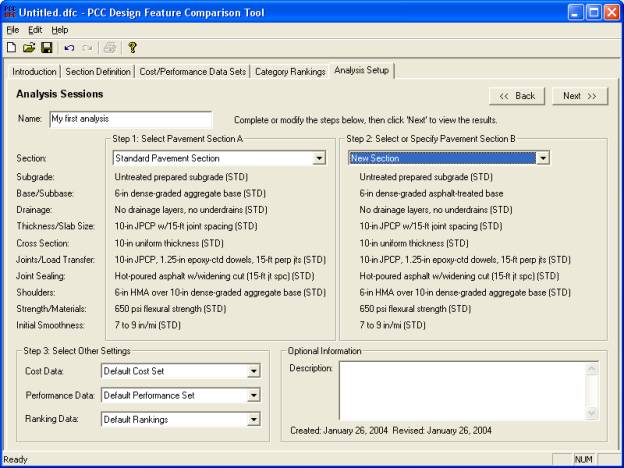
Figure 16. Example of the Direct Comparison analysis session setup dialog box.
Section A will be reflected below the list box. Those design feature values that match those that define the Standard pavement section (see table 21) are indicated by the "(STD)" that follows the feature description.
The second step in defining the Direct Comparison analysis session is the selection of the second pavement section (Section B) that will be compared to Section A. Section B may be defined by one of two methods:
The last required step of the Direct Comparison analysis involves defining the nonvarying data collection modules contained in the Step 3: Select Other Settings area. This involves selecting a cost data set, performance data set, and category ranking set from their respective list boxes. The items in each of these list boxes are those that are available in their respective master lists. Therefore, to see the detailed make up of a particular named data collection module, visit the appropriate tab and select that item from the corresponding master list.
The final section of this direct analysis dialog is an area labeled Additional Information. The Description input box is provided for users who would like to enter text that describes the focus of a given analysis session (note: entering text in this input box is completely optional). The second part of this additional information area is the displayed analysis session Creation Date.
In a Sensitivity Analysis session, various analysis scenarios are considered, and the resulting cost, performance, and LCC results are compared for all scenarios. When you create a new (or edit an existing) Sensitivity Analysis session, the dialog box presented in figure 17 is displayed. The controls on this dialog box lead the user through a series of steps that will complete the setup of a Sensitivity Analysis session. Each of the specific controls on this page is described in detail in this section.
To change the name of the current Sensitivity Analysis session, enter the new name in the Name input box. Note: The name displayed in the input box is the name that will be displayed in the Sensitivity Analysis session's master list.
The first step in defining a Sensitivity Analysis session is the selection of a principal pavement section that is used as the basis of the analysis. If multiple pavement sections are being compared, it is to this principal section that all pavement sections in the series are compared. For the other sensitivity analysis types that investigate the use of different cost data sets, performance data sets or category ranking sets, the principal pavement section is held constant throughout all defined analysis scenarios.
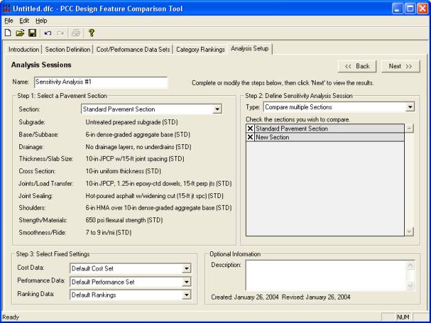
Figure 17. Example of the Sensitivity Analysis session setup dialog box.
To define the principal section, select a named pavement section from the list box within the area labeled Step 1: Select a Pavement Section. The named pavement sections contained in this list box are those stored in the Pavement Section Master List. When you select a section from the list, the design category values associated with chosen section are reflected below the list box.
After selecting a principal pavement section, you must next select the specific type of Sensitivity Analysis you wish to conduct, as well as set the parameters that define the analysis. To accomplish these tasks, use the controls provided in the frame titled Step 2: Define Sensitivity Analysis Session. Specifically, the five different dimensional analysis choices contained in the Type drop-down list box are the following (note: each of these was defined earlier in this chapter):
Upon selecting one of these analysis types, you will be provided with a list of related available items (i.e., pavement sections or cost, performance, or category ranking data sets) that can be included in the analysis. By default, all available items are initially included in the analysis. Included items are indicated by an "X" placed in the box to the left of the item's name. To exclude an item from the analysis, simply click on the associated box that contains an "X." To include a previously excluded item in the analysis, click on the empty box to again display the "X."
To illustrate this analysis setup process, figure 18 shows an example in which the user has selected a 2-dimensional analysis in which both cost and performance data sets will be compared simultaneously. Specifically, the defined analysis will investigate all of the analysis scenarios representing the different combinations of one cost set (My Cost Set) and all three available performance data sets.
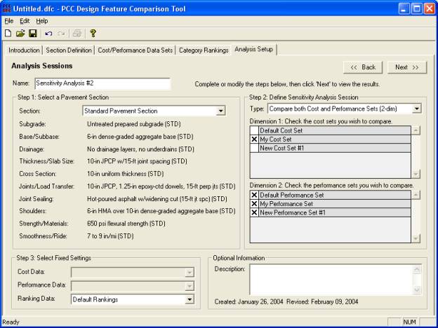
Figure 18. Example of a Sensitivity Analysis session comparing both cost and performance data sets.
The last required step of the Sensitivity Analysis setup involves the definition of the nonvarying data collection modules contained in the Step 3: Select Fixed Setting area. This involves the selection of those data collection modules that remain constant throughout the Sensitivity Analysis. To define these items, select the appropriate named item from each provided list box. The items in each of these list boxes are those that are available in their respective master lists. Therefore, to see the detailed makeup of a particular named data collection module, visit the appropriate tab and select that item from the corresponding master list.
The final section of this direct analysis dialog is an area labeled Additional Information. The Description input box is provided for users who would like to enter text that describes the focus of a given analysis session (note: entering text in this input box is completely optional). The second part of this Additional Information area is the displayed analysis session Creation Date.
The results of the current defined analysis session are summarized into a customizable output report that may be reviewed within the software. To view the results from an analysis session, click the ![]() button after you have defined the inputs for the three required steps of the analysis session setup process. The remainder of this chapter introduces the specific output reports associated with the Direct Comparison and Sensitivity Analysis session types.
button after you have defined the inputs for the three required steps of the analysis session setup process. The remainder of this chapter introduces the specific output reports associated with the Direct Comparison and Sensitivity Analysis session types.
By default, all of the available Direct Comparison analysis results are presented in the summary report (i.e., the Full Report format). However, if you are only interested in viewing specific summary tables, you may choose the Basic Tables Only option. Selecting this option allows you to customize the simplified output report by choosing to view one or more of the following summary tables:
More details on both the Full Report and Basic Tables Only reporting options are discussed separately below.
To view all of the details associated with the conducted Direct Comparison analysis, click the Full Report check box when analysis results are displayed (see figure 19). Specifically, the many different sections that are included in the full report include the following:
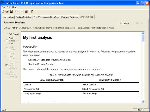
Figure 19. Example of a Full Report summary resulting from a Direct Comparison analysis.
To print the defined output report, use the Print option included under the File menu or the Print toolbar button.
The Basic Tables Only report option allows you to build a simplified version of the output report (see figure 20). Only tables selected by the user (indicated by the check boxes) are displayed in the output report with limited explanatory text.
As with a Direct Comparison analysis, Sensitivity Analysis results are by default presented in a full report format (i.e., Detailed Results). However, if you are only interested in viewing a summary table of the cost and performance results associated with each analysis scenario included in the analysis session, you may deselect the Detailed Results check box. Both the detailed results and simplified summary reports are discussed separately below.
To view all of the details associated with the conducted Sensitivity Analysis session, the Detailed Results check box needs to be selected (see figure 21). The detailed report provides many of the lower level calculations associated with each analysis scenario. Specifically, the detailed Sensitivity Analysis report contains the following three main sections:
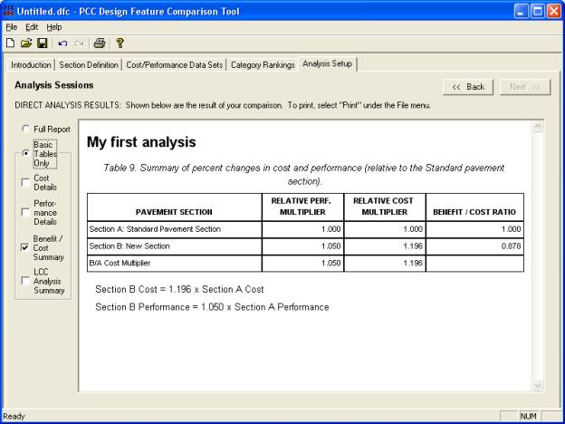
Figure 20. Example of the Basic Tables Only output report resulting from a Direct Comparison analysis.
To print the defined output report, use the Print option included under the File menu or the Print button on the toolbar.
If you choose to deselect the Detailed Results check box, you will only view an overall summary table of results associated with the conducted Sensitivity Analysis session. Each row of the table summarizes the relative performance multiplier, relative cost multiplier, and benefit/cost ratio associated with each included analysis scenario. Note: A detailed explanation of these multipliers and the benefit/cost ratio was provided in the Direct Comparison Analysis-Full Report section.
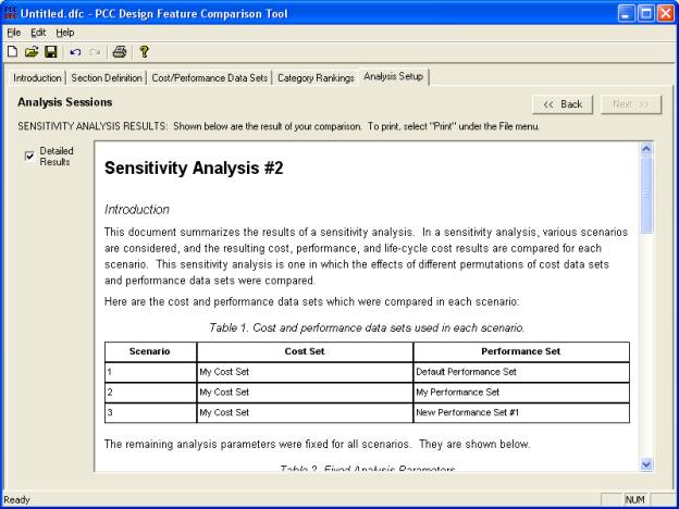
Figure 21. Example of a Detailed Results summary table output resulting from a Sensitivity Analysis session.

