Computer-Based Guidelines for Concrete Pavements Volume I-Project Summary

Previous | Table of Contents | Next

CHAPTER 3. INFORMATION SEARCH AND MODEL SELECTION

3.1 Introduction

As was briefly discussed in the introduction to this report, the HIPERPAV system has already proved successful in simulating early-age behavior of JPCP. However, although many of the models incorporated when HIPERPAV was originally developed were considered to be the best options at the time, new developments are now available that could potentially increase the accuracy of prediction. Some examples include the findings from a cement and admixtures characterization study recently conducted by the University of Texas at Austin and improved models for prediction of creep-relaxation in the early-age.^(1,2,3) Furthermore, previous validation and implementation efforts have made it possible to identify areas that may require of model enhancements, such as a better characterization of the concrete creep-relaxation effects at early ages and improved shrinkage models.

In addition, the systems approach used in HIPERPAV makes it ideal for expanding its capabilities to include new modules for prediction of JPCP long-term performance as a function of early-age behavior. Incorporating new modules for predicting early-age behavior of other pavement types such as CRCP is similarly possible.

Finally, a number of studies oriented to enhance the performance of concrete pavements have been identified to be compatible with the function of the HIPERPAV system, and therefore also may be incorporated.

To accomplish the objectives for this project, an information search first was conducted to identify models in each of the above categories. In this chapter, the information review results are described. The chapter is divided into three sections:

1. Literature search (section 3.2).
2. Model identification and selection (section 3.3).
3. Review of FHWA studies for potential incorporation into HIPERPAV II (section 3.4).

3.2 Literature Search

This section describes the literature review efforts made to identify theoretical models developed to date in each of the following four categories:

• Currently available early-age behavior simulation software similar to HIPERPAV.
• General early-age behavior models.
• JPCP performance models.
• CRCP early-age behavior models.

The following sections describe the literature review for each of the above categories. A detailed annotated bibliography on the primary references reviewed during the information search performed in this study is provided in volume III, appendix A of this report series.

3.2.1 Currently Available Early-Age Behavior Simulation Software Similar to HIPERPAV

Besides HIPERPAV, four other software programs that can similarly predict the early-age behavior of concrete have been identified. These include DuCOM®, HYMOSTRUC®, Quadrel®, and 4C Temp & Stress®. HYMOSTRUC and Quadrel focus on developing the adiabatic hydration curves for concrete. DuCOM and 4C Temp & Stress are more robust FEM programs that calculate the state of stress in early-age concrete structures. These programs are similar in some aspects to HIPERPAV, but also have differences in theory and application. DuCOM, HYMOSTRUC, Quadrel, and 4C Temp & Stress are summarized in volume III, section A.1 of appendix A in this report series. A review of these models has helped in identifying possible improvements in the HIPERPAV software for characterization of early-age behavior. The section below describes specific models identified for possible incorporation into HIPERPAV.

3.2.2 General Early-Age Behavior Models

The early-age properties of concrete are significantly influenced by the climatic conditions and temperatures, as well as by the concrete mix components. For this purpose, a literature review of early-age concrete properties was completed. The properties that are addressed include:

• Concrete hydration.
• Concrete maturity.
• Drying shrinkage of concrete.
• Moisture transport in concrete.
• Set time of concrete.
• Creep.

A literature search was also performed for concrete thermal properties including: CTE, thermal conductivity, specific heat, thermal diffusivity, convection, surface emissivity, and solar absorptivity.

The literature review on early-age concrete properties is summarized in volume III, section A.2 of appendix A in this report series.

3.2.3 JPCP Performance Models

The literature review of JPCP models contained three categories. The first category was a literature review on pavement structural models for prediction of pavement response as a function of temperature, moisture, and traffic loading. The second category was a literature review on available climatic models that can be used in conjunction with the structural models to account for climatic conditions at the time of pavement curing and also over the years as the pavement is subjected to long-term usage. In the third category, a number of JPCP performance models were investigated. A literature review on faulting, transverse cracking, spalling, and JPCP roughness was conducted for this purpose. In HIPERPAV, it is preferable to use mechanistic models that have been calibrated and validated with actual experimental data. Information on the above three categories is presented in volume III, section A.3 of appendix A in this report series.

3.2.4 CRCP Early-Age Behavior Models

A literature review on CRCP early-age behavior also was conducted. From this effort, a number of references have been compiled, and models were identified describing the early-age behavior of CRCP. An additional effort was made to identify references on CRCP long-term performance. References on CRCP early-age behavior and CRCP long-term performance are summarized in volume III, section A.4 of appendix A in this report series.

3.2.5 Electronic Database and Search Tool

To help the project team coordinate references, performance data sources, and other aspects of the project, an electronic database and associated search tool were developed.

The search tool, a Microsoft Windows application, allows the user to search by specific categories related to PCC, JPCP, CRCP, and bonded concrete overlays (BCO). A screen capture of the computer program is shown in figure 2. In addition, the user can refine the search by typing title, author, or keywords into the three text boxes just above the results window. If the user does not know the exact spelling of a word, partial entries in these boxes will produce matches that contain the text string somewhere in the reference database entry.

The tool may be of use to those who are interested in learning more about concrete pavements. For this reason, and to enhance the reliability and acceptability of the results of this research project, this database and search tool has been coupled with the final software product from this study.

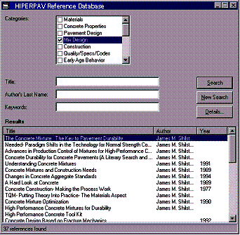
Figure 2. Microsoft Windows screen capture of database search tool.

3.3 Model Identification and Selection

This section summarizes the general early-age behavior models, JPCP performance models, and CRCP models identified. A description of model selection is provided, followed by a brief evaluation of each model. The models finally selected for incorporation in the HIPERPAV II system are fully documented in volume III, appendix B of this report series.

3.3.1 Model Approach

In this new set of guidelines, a mechanistic approach is used to describe the existing link between early-age behavior and long-term performance. Traditionally, three classes of theoretical models have been used in the pavement engineering field to predict long-term pavement behavior and performance: empirical, mechanistic, and a hybrid: mechanistic-empirical.

3.3.1.1 Empirical Models

Empirical models are based on experimental data collected from field studies. These models are considered valid only within the limited range of data collected. If, for example, the environmental, material, or loading conditions are outside the boundaries of the study, then the model is no longer applicable. A new model will have to be developed for the new conditions. For this reason, empirical models cannot be applied to all situations.

3.3.1.2 Mechanistic Models

Mechanistic models do not have the same limitations as empirical models. Mechanistic models are based on the mechanics of the materials and physics behind the problem. With mechanistic models, stress, strain, or resulting deflections are determined to explain the influence of internal or external forces over the pavement system. Using the theoretical mechanistic equations, pavement performance can be predicted.

3.3.1.3 Mechanistic-Empirical Models

The empirical approach of pavement performance prediction is a two-step process. From the input parameters, the LTPP (distress) history can be predicted. This process is illustrated in figure 3. However, this method bypasses four key steps that the mechanistic approach takes into account. The mechanistic method accounts for the material characterization (e.g. strength development of the concrete). Pavement response is then predicted (e.g., stresses development in the slab due to temperature loading). Then, pavement behavior is assessed (e.g., permanent deformation of the pavement slab as a result of curling/warping effects). Finally, the pavement distress is predicted (e.g., transverse cracking). From this, the distress history as a function of time can be generated.

Although mechanistic models more clearly determine the process of pavement behavior and performance, theory, by itself, has not proven sufficient for an accurate analysis of pavements. Therefore, the observed performance must be used with the mechanistic model as part of calibration. Consequently, the models used in pavement performance prediction are commonly termed mechanistic-empirical models. Mechanistic-empirical models are defined as analytical models calibrated with field observations that may be used to predict pavement performance reliably.

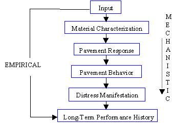
Figure 3. Schematic of empirical and mechanistic solutions for prediction of pavement distress.

There are at least three primary benefits to successfully applying mechanistic-empirical models in design. These are:

• Increased design reliability.
• Ability to predict specific types of distresses.
• Ability to extrapolate from limited sets of field and laboratory results.

Mechanistic-empirical models can be used to provide better pavement performance predictions. With these models, the effect of new parameters can be assessed, such as new loading or materials. Available materials are better utilized, and improved diagnostic techniques are available, leading to an understanding of why a pavement is performing better or worse than expected. Improved modeling of aging distresses, weather, subbase erosion, and the benefits of improved drainage also can be modeled effectively with mechanistic-empirical models.

The concepts behind development of a regression (empirical) model are shown in figure 4. Using the observed points, a regression curve is fit through them. The regression curve can be used to extrapolate beyond the physically measured values for prediction purposes. However, it is this extrapolation that demonstrates the potential for inaccuracy of regression models.

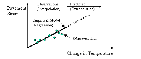
Figure 4. Use of empirical (regression) model for prediction of concrete strains.

In figure 5, an example of the analytical (mechanistic) solution versus the regression solution is shown. The slope of the analytical model is not necessarily the same as that of the regression curve. For this reason, when both are used in the prediction side of the plot, the difference from the regression model is apparent.

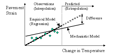
Figure 5. Use of empirical and analytical (mechanistic) model for prediction.

With the collection of additional data, the analytical model can be calibrated for specific sites, resulting in a mechanistic-empirical model. This further increases the accuracy of the analytical model (see figure 6).

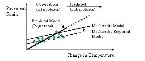
Figure 6. Use of empirical and calibrated analytical (mechanistic-empirical) model for prediction.

In summary, empirical models do not have the same indepth analysis as mechanistic models; instead, they directly relate input to LTPP based on site-specific data. Mechanistic models are the result of a five-step process to relate input to material characterization, pavement response, pavement behavior, distress prediction, and long-term performance history. Without calibration, mechanistic models are not site specific like the empirical models. Instead, these models account for the physical processes behind LTPP. Despite the shortcomings of the empirical data, it is still needed to calibrate the mechanistic models. The use of mechanistic-empirical models is preferred in pavement design and analysis.

3.3.2 Selection Criteria

Five primary factors have been considered in the selection of models for incorporation in HIPERPAV II, namely:

• Type of approach.
• Status of development.
• Calibration/validation.
• Inputs.
• Outputs.

These selection criteria are described below:

1. Type of approach: The HIPERPAV system has been recognized for providing a mechanistic approach to the analysis of early-age behavior of JPCP during the first 72 hours after construction. The advantages of mechanistic models, as compared to empirical models, were provided in section 3.3.1. The selection of models for analysis of JPCP and CRCP should favor mechanistic or mechanistic-empirical models. Also, as stated in the objectives of this project, the most important factor considered when selecting JPCP long-term performance models was the effect that early-age behavior factors had on long-term performance. Section 3.3.4 expands on the importance of early-age behavior factors on long-term performance.
2. Status of development: Some of the identified models may be conceptual, or currently under development. As the scope of this project does not include the resources for developing new models, caution must be used in selecting models that are not fully developed.
3. Calibration and validation: Calibration and validation of the available models was also an important factor to consider in model selection. Some limited validation of the models selected was performed within the scope of this project. However, it was desired that the models selected had undergone at least some calibration to warrant their selection, and to be certain that the model had sound logic in its development.
4. Inputs: One of the objectives of the HIPERPAV system is to be as practical as possible. Models that require inputs that may be difficult to obtain, or not readily available to the average user, were considered undesirable.
5. Outputs: The selection of pavement early-age behavior models will eventually help to assess long-term performance. Therefore, these models should provide the necessary information required by existing long-term performance models.

3.3.3 General Early-Age Behavior Models

The early-age behavior models used in HIPERPAV I for stress and strength prediction are described in detail in previous reports.⁽⁴⁾ The models identified here are improvements to some of those models, which predict:

• Cement hydration.
• Concrete temperature.
• Concrete moisture.
• Shrinkage.
• Concrete creep.
• Subbase restraint.
• Thermal gradients.

3.3.3.1 Concrete Hydration Models

From the literature review, several models were identified as candidates to incorporate into HIPERPAV II for expanding and improving the current hydration model. Table 2 lists the identified models, including a summary of advantages and disadvantages for using each of the models. Inputs required, outputs, validation, and need for further development are also identified.

During this project, the research team closely followed the development of hydration models conducted by the University of Texas at Austin under a research project with the Texas DOT.⁽¹⁾ The models developed by Schindler were selected for use in HIPERPAV II, because they could be adapted with relative ease and are practically the only hydration models available validated with U.S. cements. A detailed description of these models is provided in volume III, appendix B of this report series.

3.3.3.2 HIPERPAV II Finite-Difference Temperature Model

In HIPERPAV I, a one-dimensional FEM technique was used, but this procedure has proven to be a computational burden and may not be appropriate for the large number of time-steps involved in long-term analyses. The finite-difference method (FDM) is another numerical technique that is available to solve the transient heat transfer problem. In this study, the previous FEM procedure for heat transfer analysis was replaced with an FDM after extensive calibration and validation. The finite-difference model FDM model is used for both early-age and long-term predictions of concrete temperature. A description of this model is provided in volume III, appendix B of this report series.

3.3.3.3 Models for Characterization of Concrete Moisture

Many of the models in HIPERPAV I include terms for the moisture state in the PCC. The current moisture model in HIPERPAV I assumes that the moisture gradient varies uniformly from the surface of the pavement to near 100 percent at the center of the slab and below. Although incorporating a mechanistic-based moisture transport model is outside of the scope of this project, an effort was made to improve the moisture characterization. This step included integrating moisture terms into the most sensitive models such as the strength, shrinkage, and warping models.

An improvement to the current model was considered, based on the model proposed by Parrott for PCC slab moisture prediction.⁽⁵⁾ Zollinger has proposed a modification to the Parrot model to account for the effect of curing.⁽⁴⁾ The curing material is assigned an equivalent thickness of concrete. This additional thickness of concrete on top of the slab is assumed to mitigate the moisture loss from the pavement surface. This equivalent thickness was proposed based on an empirical data fit from laboratory data collected to derive the moisture gradient through the slab depth. Rasmussen proposed a modification to the Zollinger model.⁽⁴⁾ Following the same methodology, the revised model increases the depth of the slab by the equivalent thickness, and derives the resulting moisture gradient. This can be seen graphically in figure 7.

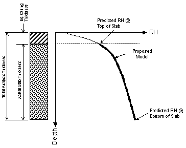
Figure 7. Graphical representation of revised Rasmussen-Zollinger-Parrot model.

Although it is believed that the modified Parrott model would improve the moisture characterization in HIPERPAV, a careful calibration and validation process of the model would have been required before integrating it into the HIPERPAV system. However, validating this model was outside the scope of this project.

3.3.3.4 Shrinkage Models

Two shrinkage models were identified for incorporation into HIPERPAV II: a drying shrinkage model with better materials characterization than the one previously used; and an autogenous shrinkage model for low water-cement ratios.

Although developed later than the previous Reunion Internationale des Laboratoires D'essais et de Recherches sur les Materiaux et les Constructions (RILEM) B₃ model used in HIPERPAV I, the Bazant-Panula (BP) drying shrinkage model incorporates more empirical material dependencies.^{(6, 7)} One of these empirical dependencies is the influence of the aggregate volume fraction on final shrinkage, on which drying shrinkage is believed to be greatly dependent. It accounts for the total aggregate (coarse + fine)-to-cement ratio by weight, the coarse aggregate-to-fine aggregate ratio by weight, and the sand-to-cement ratio by weight. These two models are very similar; however, the B₃ model does not account for these aggregate contributions. Predictions of the BP model and the B₃ model were compared, and it was found that the BP model was better able to predict the shrinkage of concrete specimens of various mix designs. The drying shrinkage model in HIPERPAV II was therefore updated, from the RILEM B₃ model previously used to the BP model. This model is described in volume III, appendix B of this report series.

Table 2. Hydration models identified for possible incorporation in HIPERPAV II.

MODEL	PROS	CONS	VALIDATION	INPUTS	OUTPUTS	DEVELOPMENT
Schindler Hydration Models(1)	-Practical -Can accommodate any cement type -Accounts for fineness	-Empirical -Few tests results on mineral admixtures	Yes, laboratory and limited field conditions	-Cement composition -Water-cement ratio -Mineral admixtures replacement	-Degree of hydration -Activation energy -Set time	Complete
Swedish CCRI*(8)	-Practical -Well established -Can accommodate any cement type -Data for many mix designs available	-Effect of moisture not modeled -Effect of cement fineness cannot be modeled -Few test results on mineral admixtures	Yes, under laboratory conditions	-Mix proportions -Curing temperature -28-day strengths -Cement type	-Compressive strength -Modulus of elasticity -Poisson's ratio -Creep adjusted modulus -Degree of hydration -Total heat of hydration	Mostly complete Creep models not completed
Dispersion Model(9)	-Account for cement fineness -Simplicity -Recognized and accepted	-Limited data available on particle size distribution.	Partially	- Mean particle size - Rate constant	-Degree of hydration -Strength vs. maturity	Complete
Hyperbolic Model(10)	-ASTM** standard model	-Requires conversions from compressive to tensile	Yes	-Final strength -Activation energy -Set time	-Strength gain	Complete
HYMOSTRUC(11)	-Accounts for effect of moisture -Accounts for effect of moisture	-Microstructure development is modeled -Effects of mineral and chemical admixtures are not addressed -Large investment in development time	Yes	-Cement composition -Particle size distribution -Water/cement ratio -Initial curing temp -Adiabatic testing -Concrete strength	-Degree of hydration -Temperature -Pore structure -Strength -Stress -Risk of cracking	Complete, but constantly being modified and expanded
DuCOM(12)	-Accounts for effect of moisture -Modeling of deterioration mechanisms (corrosion and sulfate attack)	-Microstructure development is modeled -Large investment in development time -Moisture model needs improvement	Yes	-Mix proportions -Particle size distribution -Initial curing temperature -Chemical composition -Structural dimensions	-Porosity distribution -Strength -Moisture distribution -Shrinkage, creep -Thermal strains -Concentration of harmful agents	Complete, but constantly being modified and expanded Moisture model in progress
Rahhal and Batic(13)	-All combinations of mineral admixtures considered	- Argentinean cement types - Empirical model	Yes, empirical	-Mineral admixture replacement level -Cement heat of hydration	-Blended cement total heat of hydration	Complete

*CCRI = Swedish Cement and Concrete Research Institute
**ASTM = American Society for Testing and Materials

Concrete paving mix designs continually are being developed with lower water-to-cementitious materials ratios (w/cm). It is not uncommon for the w/cm to drop below 0.40. When this occurs, there is not enough water available in the fresh concrete mixture to allow for the complete hydration of the unhydrated cement grains. Two forms of shrinkage are apparent: drying shrinkage (already included in the HIPERPAV I prediction) and autogenous shrinkage. Autogenous shrinkage is a low w/cm phenomenon, and it cannot be ignored in these instances. For example, total shrinkage of a concrete mixture having a w/cm of 0.30 can be 50 percent autogenous shrinkage and 50 percent drying shrinkage. Neglecting autogenous shrinkage would significantly underestimate the concrete's shrinkage in the field; therefore, identifying an autogenous shrinkage model was necessary. The autogenous shrinkage model identified for incorporation in HIPERPAV II is the one developed by Jonasson and Hedlund.⁽¹⁴⁾ A detailed description of this model is presented in volume III, appendix B of this report series.

3.3.3.5 Concrete Creep and Relaxation

Efforts were also made to investigate further the extended triple power law creep/relaxation model identified from previous efforts. Although it was anticipated that such a model would require extensive calibration and validation efforts, an initial model evaluation was conducted during this project.

This model is developed from the double power law and the triple power law.^{(14, 15)} The double power law is perhaps the most well known compliance function, and has been used by many authors, because it is based on extensive laboratory test results. The triple power law was developed to more accurately describe the long-term creep. Neither the double nor the triple power laws were calibrated for loading at early ages, and they were not intended to predict creep for young concrete.⁽²⁾ Westman estimated that the double and triple power laws are only valid for loading ages larger than about 2 days.⁽³⁾ Therefore, the triple power law was adjusted first by Emborg, and then by Westman, to account for loading at ages less than about 2 days.^{(2, 3)} The extended triple power law, as documented by Westman, provides good agreement with early-age test data, and accounts for all the factors that could influence the time dependent deformation, such as:

• Concrete age at setting.
• Concrete age at loading (which is most important).
• Applied stress level.
• The influence of varying temperature.

The model definition for the creep/relaxation model based on the extended triple power law is provided in volume III, appendix B of this report series.

3.3.3.6 Nonlinear Restraint Model

Recognizing the nonlinear restraint effect imposed by some subbases, such as hot-mix asphalt subbases, a nonlinear model was also included in addition to the current linear one to provide for the characterization of such behavior. The nonlinear restraint model is described in volume III, appendix B of this report series.

3.3.3.7 Nonlinear Thermal Gradient Model

Finally, recognizing that thermal gradients through the slab depth are nonlinear for the most part, the model developed by Mohamed and Hansen was included to determine an equivalent linear gradient as a function of a nonlinear one.⁽¹⁶⁾ This model is described in volume III, appendix B of this report series.

3.3.4 JPCP Performance Models

To analyze the behavior of JPCP and to predict JPCP distress development as a result of traffic loading, analytical models were selected. As stated in the objectives of this project, the most important factor considered when selecting these analytical models was the effect that early-age behavior factors had on long-term performance. Researchers found the size of the joint opening, curling and warping of the slab, and moisture loss at early ages in JPCP to be some of the primary early-age indicators of the pavement's long-term performance. A brief description of primary early-age behavior factors is given in the following bullets. More detailed information on these factors can be found in volume II of this report series:

• Joint opening controls the LTE across the joint, which controls how well the JPCP will perform over time. Large joint openings may lead to JPCP spalling, faulting, and transverse cracking. The joint opening at early ages is controlled primarily by the effect that temperature and moisture changes have on pavement and subbase properties such as concrete CTE, drying shrinkage, and subbase restraint. Joint opening varies with the daily temperature cycles due to changes in the pavement's thermal conditions. Drying shrinkage, CTE, and pavement length also affect the joint opening. To control the joint opening to acceptable levels, properly curing the pavement at early ages is of paramount importance.
• Evaporation of bleed water at the concrete surface is governed by the concrete temperature and climatic conditions such as windspeed, relative humidity, and air temperature. However, at any point during the early age of the pavement, the loss of moisture in concrete pavements will also be a function of the moisture transport characteristics of the concrete, the water available in the mix, and in particular, the water that has not been used for hydration. Moisture gradients usually develop in concrete pavements due to the loss of moisture to the environment. Under conditions where significant moisture is lost to the environment, critical moisture gradients may develop in the slab, leading to a reduction in the strength of the concrete at the slab surface, plastic shrinkage, and cracking. Moisture loss may later result in delamination and spalling of the concrete surface.
• The temperature gradients during the early age are a function of the environmental conditions and the heat concrete hydration. The initial thermal gradient in the slab at set will influence the curling shape of the slab. Built-in curling is a term used for the curling state that develops at set and that later influences the curled shape of the slab as the thermal gradient is subsequently modified by the hydration process and climatic conditions. In general, when concrete sets, the temperature through the slab is generally not uniform, but rather is a function of the climatic conditions, the heat of hydration, and curing methods. Built-in curling may later translate into faulting and cracking problems as the level of stresses developed in the pavement slabs is increased as a function of traffic loads and long-term daily and seasonal climatic conditions.

A discussion of JPCP performance models that were identified in the literature search of this project is provided in this section, along with a discussion on the models that were finally incorporated in HIPERPAV II. The models are divided into four categories:

1. Environmental.
2. Long-term materials properties models.
3. Structural behavior models.
4. Distress prediction models.

3.3.4.1 Environmental Models

Table 3 provides a summary of the climatic models considered, including model basis, advantages, and disadvantages. The models selected for incorporation in HIPERPAV II were the FDM model developed under this study, and the subgrade moisture model by Lytton.⁽²³⁾

The FDM is used to predict long-term concrete temperatures. The selection of this model is previously discussed in section. The FDM model is described in detail in volume III, appendix B of this report series.

The moisture model provides a simple method to predict the average monthly moisture content in pavement base materials using site-dependent climate conditions, soil data, and some pavement geometry. This model is described in detail in volume III, appendix B of this report series.

3.3.4.2 Long-Term Materials Properties Models

Mechanical properties used for long-term PCC characterization include modulus of elasticity and any of the following three strengths: tensile, flexural (modulus of rupture), or compressive. During the pavement life, the PCC slab is exposed to various stresses, such as curling and warping stresses, thermal axial stresses, and wheel load stresses. In the long term, one of the major failure modes is cracking due to fatigue. This generally has been found to be a function of the tensile stress to strength ratio at the bottom of the layer, implying that tensile strength is a significant characterization property. Unlike most concrete structures, JPCP does not rely on steel to withstand tensile stresses and therefore typically is designed using a specified tensile strength. Because concrete is much weaker in tension than in compression, tensile strength is the most critical strength characteristic.

The elastic modulus is an estimate of the slope of the stress-strain curve in the elastic region and a good indicator of the overall structural stiffness of the concrete. Because stresses and strains are related through the elastic modulus under assumptions of linear elasticity, it is important that this property be characterized.

Although conversion coefficients for the different strength types are user-defined in HIPERPAV II, default conversion models were investigated. The model sources identified are:

• Conversion relationship between third point modulus of rupture (MOR) and splitting tensile strength developed by Melis et al.⁽¹⁷⁾
• Conversion relationship between third point MOR and center point MOR developed by Carrasquillo and Carrasquillo.⁽¹⁸⁾
• Conversion relationship between third point MOR and compressive strength developed by Raphael.⁽¹⁹⁾
• Conversion relationship between compressive strength and modulus of elasticity recommended by the American Concrete Institute (ACI).⁽²⁰⁾

In addition, the long-term strength gain after 28 days was investigated. Long-term strength and stiffness models recommended by the CEB/FIP [2] Model Code 1990 were incorporated.

A detailed description of each of the above models is presented in volume III, appendix B of this report series.

3.3.4.3 Structural Models (Load TransferEfficiency, and Midslab Stress and Deflection Models)

To predict accurately the response of a rigid pavement due to external wheel loads, a model is needed to assess the behavior of the pavement structure in the vicinity of discontinuities such as cracks and joints. Several structural response models based mainly on FEM modeling were identified. A summary of their advantages and limitations is presented in table 4. Initially, a FEM model such as KENSLABS had been proposed to predict slab stresses due to traffic loading for use in the pavement performance cracking models in HIPERPAV II.⁽²¹⁾ However, due to the computational burden of the FEM model and because the cracking models selected are based on stresses predicted with Westergaard formulations, a structural model that accounts for LTE between slabs was developed under this study and was considered more appropriate for this purpose. The LTE, stress, and deflection models selected for incorporation in this study are presented in volume III, appendix B of this report series.

3.3.4.4 Distress Models

As previously mentioned in section 3.3.2, several criteria were considered in the selection of each individual JPCP distress model. In selecting long-term distress prediction models, the most important criterion (with respect to this effort) is that the model account for early-age indicators for distress prediction such as joint opening and/or built-in curling. Tables 5 to 9 present the JPCP distress models identified in the literature. For these tables, the "Model Basis" category designates whether the model is mechanistic, empirical, or mechanistic-empirical in nature. Additional fields include the databases used for their development, the quality of data used in their development, model statistics, early-age modeling parameters used, and availability of required model inputs.

3.3.4.4.1 Faulting

Table 5 shows the faulting models identified. Models for both doweled and nondoweled pavements were investigated. The models selected are those developed by Smith et al. reported in FHWA-RD-89-137.⁽²²⁾ Selecting the same model source for both doweled and nondoweled pavements was important to avoid inconsistencies in predicting faulting distress under each condition. In addition, these models include an input for joint opening, which is considered an important indicator needed to relate the performance of the pavement to early-age conditions. Selection of these models was also reinforced because they are mechanistic-empirical in nature. Besides joint opening, they account for traffic loading, environmental conditions, support conditions, pavement structure, and the presence of dowels. Finally, these models were developed using the combined Concrete Pavement Evaluation System (COPES) and Performance/Rehabilitation of Rigid Pavements (RIPPER) databases with a large data set of pavement sections in a variety of environmental regions (wet-freeze, wet-no freeze, dry-freeze and dry-no freeze) in the United States.⁽²²⁾

These faulting models originally were developed and calibrated based on a unique definition of joint opening. The joint opening prediction made by HIPERPAV II is based on a different approach than the FHWA model. The FHWA model is a closed-form and rather simple prediction, while the model in HIPERPAV II is based on a more sophisticated FDM-based analysis. Therefore, to use the joint prediction made by HIPERPAV II in predicting long-term faulting, a submodel was developed to convert the HIPERPAV II-predicted joint opening to the joint opening parameter used in the FHWA faulting model.

A detailed description of the faulting models and development of the HIPERPAV II joint opening conversion model are presented in volume III, appendix B of this report series.

Table 3. Climatic models.

Model	Model Basis	Pro	Con
HIPERPAV II	M-E*	- Able to predict the early-age behavior of PCC 72 hours after construction - Transient FDM temperature core - Accounts for climatic conditions	- Some empirical assumptions
Lytton(23)	E**	- Fast run-time - Limited validation	- Simplistic model with empirical assumptions
ICM(23)	M-E	- Predicts moisture and temperature profiles in pavement structures	- Moisture model still under development - Slow run-time

*M-E = Mechanistic-Empirical
**E = Empirical

Table 4. Structural behavior models.

Model	Model Basis	Pro	Con
KENSLABS(21)	M	- FEM-based - User-defined dimensions - Two layers (bonded/un) with same/different material properties - Liquid/solid subgrade - Uniform/nonsupport to account for erosion - Multiple slabs with load transfer - Warping/curling with load response - Arbitrary loading conditions-wheel loading - Arbitrary shoulder conditions - Nonuniform slab/shoulder thickness	- Large amounts of computer storage
ILLI-SLAB (24)	M	- FEM-based - User-defined dimensions, any number of slab arrangements, layer bonding - Two layers (bonded/un) with same/different material properties - Liquid/solid subgrade - Uniform/nonsupport to account for erosion - Multiple slabs with load transfer - Warping/curling with load response - Arbitrary loading conditions, axle configurations - Arbitrary shoulder conditions - Nonuniform slab/shoulder thickness	- Large amounts of computer storage - Poorly conditioned source code
ISLAB 2000(25)	M	- Improvement to ILLI-SLAB	- Source code not available
JSLAB(26)	M	- FE used to compute critical stresses and deflections	- Stiffness matrix reportedly not correct - Based on early version of ILLI-SLAB
LTE, stress, and deflection	M	-Fast computations -Predicted stresses compatible with selected midslab cracking model inputs	-Simplistic closed-form solution

3.3.4.4.2 Midslab and Corner Cracking Models

Tables 6 and 7 present the midslab and corner cracking models identified during the literature search respectively. The models selected were those developed by Yu et al. in FHWA-RD-95-111 and the stress adjustment models developed by Lee and Darter and Lee et. al. (See references 27, 28, 29, and 30.) The midslab cracking model is based on Westergaard stresses. Using this model, joint opening, LTE, and built-in curling can be accounted for by using the LTE, stress, and deflection model developed in this study. The accumulated fatigue damage is predicted, as is the percentage of cracked slabs, in both the longitudinal and transverse directions.

These models were selected given the following considerations:

• The model uses mechanistic components.
• The fatigue model is based on Miners Law using the Westergaard edge stress prediction model.
• By incorporating the LTE, stress, and deflection models, stress can be calculated for typical slab configurations, load transfer devices, and joint opening; these can be included as a predictor variable for the stress state at any given time as a function of climatic conditions using the HIPERPAV II joint opening prediction model.
• By employing the stress adjustment factors developed by Lee and Darter, the model can be adapted to use load spectra or 18-kip Equivalent Single Axle Loads (ESAL).
• A relative good fit of a comprehensive database was used for the midslab cracking model validation.

More details on the selection and a detailed description of the midslab cracking models are provided in volume III, appendix B of this report series.

No corner cracking model was selected for incorporation in HIPERPAV II because the LTE model is one-dimensional and could not account for stress transfer efficiency on both directions as a function of joint opening near the corner location. The corner cracking models identified did not account for joint opening or were based on FEM runs impractical for incorporation in HIPERPAV II due to the analysis time required by the FEM.

3.3.4.4.3 Spalling Model

Table 8 shows spalling models identified. Although a number of models were identified, the difficulty to realistically account for all the factors affecting spalling distress was recognized during the TEP meetings. Since developing a new spalling model was out of the scope of this project, it was decided not to include a spalling distress model in HIPERPAV II during this effort.

3.3.4.4.4 Roughness Model

Two common roughness indicators are the Present Serviceability Index (PSI) and the International Roughness Index (IRI). A number of models for both roughness indicators were identified in this project and are summarized in table 9. A detailed comparison of the models identified is presented in volume III, appendix B of this report series.

Table 5. Faulting models.

Models	Model Source	Model Type	Development Database	Quality of Data Used in Model Development	Model Statistics	Early-Age Modeling Parameter	Availability of Required Model Inputs
Doweled JPCP	Yu et al., 1998 FHWA-RD-95-111(27)	Mechanistic-Empirical	COPES+ with 208 more sections	Good	N = 146 sections r2 = 0.60 RSE = 0.056 mm	Dowel bearing stress	Sufficient data for 12 of 13 inputs
	Simpson et al., 1994 SHRP P-393(31)	Empirical	LTPP GPS-3 and GPS-4	Good	N = 59 sections r2 = 0.53 RMSE = 0.071 mm	None	All six inputs are available in all potential databases
	Smith et al., 1990 FHWA-RD-89-137(22)	Mechanistic-Empirical	COPES+	Good	N = 559 sections r2 = 0.67 SEE = 1.27 mm	Dowel bearing stress, Joint opening	Sufficient data for 12 of 14 inputs
Nondoweled JPCP	Yu et al., 1998 FHWA-RD-95-111(27)	Empirical	COPES+ with 208 more sections	Good	N = 131 sections r2 = 0.45 RSE = 0.86 mm	None	Sufficient data for eight of nine inputs.
	Smith et al., 1990 FHWA-RD-89-137(22)	Mechanistic-Empirical	COPES+	Good	N = 398 sections r2 = 0.81 SEE = 0.71 mm	Joint opening, Corner deflection	Sufficient data for 20 of 22 inputs
	Simpson et al., 1994 SHRP P-393(31)	Empirical	LTPP GPS-3	Good	N = 25 sections r2 = 0.55 RMSE = 1.19 mm	None	All five inputs are available in all potential databases
Doweled and Nondoweled JPCP	Titus-Glover et al., 1999 FHWA-RD-98-113(32)	Mechanistic-Empirical	LTPP	Good	N = 120 sections r2 = 0.56 SEE = 0.762 mm	Deflections of unloaded slab	Sufficient data for 9 out of 10 inputs
	Darter et al., 1985 COPES(33)	Empirical	COPES	Good	N = 259 sections r2 = 0.79 RMSE = 0.51 mm	None	Sufficient data for all seven inputs

N = number of observations
r² = coefficient of determination
RMSE = root mean-square error
RSE = relative standard error
SEE = Standard Error of the Estimate

Table 6. Midpanel cracking models.

Model Source	Model Type	Development Database	Quality of Data Used in Model Development	Model Statistics	Early-Age Modeling Parameter	Availability of Required Model Inputs
Yu et al., 1998 FHWA-RD-95-111(27)	Mechanistic- Empirical	COPES+ with 208 more sections	Good	N = 465 sections r2 = 0.91 SEE = 6.8%	None	Sufficient data available for 12 of 13 inputs
Titus-Glover et al., 1999 FHWA-RD-98-113(32)	Mechanistic- Empirical	LTPP	Good	N = 92 sections r2 = 0.64 SEE = 12%	Damage due to temperature stresses	All eight inputs are available in all potential databases
Smith et al., 1990 FHWA-RD-89-137(22)	Mechanistic- Empirical	COPES+	Good	-	None	All four inputs are available in all potential databases
Simpson et al., 1994 SHRP P-393(31)	Mechanistic- Empirical	LTPP	Good	-	None	Sufficient data available for six of eight inputs
Darter et al., 1985 COPES(33)	Mechanistic- Empirical	COPES	Good	N = 303 sections r2 = 0.69 SEE = 33.3 m/km	None	Sufficient data available for all six inputs
Lee and Darter (28, -30)	Mechanistic	n/a*	-	-	Curling

* FEM model development
N = number of observations
r² = coefficient of determination
SEE = Standard Error of the Estimate

Table 7. Corner cracking models.

Model Source	Model Type	Development Database	Quality of Data Used in Model Development	Model Statistics	Early-Age Modeling Parameter	Availability of Required Model Inputs
Lee and Lee(34)	Mechanistic	n/a*	-	-	Curling
Titus-Glover et al., 1999 FHWA-RD-98-113(32)	Mechanistic-Empirical	LTPP	Good	N = 92 sections r2 = 0.69 SEE = 9%	Damage due to temperature stresses	All eight inputs are available in all potential databases

* FEM model development
N = number of observations
r² = coefficient of determination
SEE = Standard Error of the Estimate

Table 8. Spalling models.

Models	Model Source	Model Type	Development Database	Quality of Data Used in Model Development	Model Statistics	Early-Age Modeling Parameter	Availability of Required Model Inputs
Doweled and Nondoweled JPCP	Simpson et al., 1994 SHRP P-393(31)	Empirical	LTPP GPS-3	Good	N = 56 sections r2 = 0.34 RMSE = 11.05% joints	None	All two inputs are available in all potential databases
Titus-Glover et al., 1999 FHWA-RD-98-113(32)	Mechanistic-Empirical	LTPP	Good	N = 52 Sections r2 = 0.61 RMSE = 12.0% joints	Relative humidity from month of construction, Horizontal movement of slab	Sufficient data available for 11 of 15 inputs
Senadheera and Zollinger, 1994(35, 36)	Mechanistic - Empirical	TTI	Good	-	Moisture loss from concrete surface, joint opening
Yu et al., 1998 FHWA-RD-95-111(27)	Empirical	COPES+ with 208 more sections	Good	N = 163 sections r2 = 0.76 RSE = 5.1% joints	None	Sufficient data available for all 10 inputs
Smith et al., 1990 FHWA-RD-89-137(22)	Empirical	COPES+	Good	N = 262 sections r2 = 0.59 SEE = 9.3 joints/km	None	All five inputs are available in all potential databases

N = number of observations
r² = coefficient of determination
RMSE = root mean-square error
RSE = relative standard error
SEE = Standard error of the estimate

Table 9. Roughness (ride) models.

Pavement Type	Model Source	Model Type	Development Database	Quality of Data Used in Model Development	Model Statistics	Early-Age Modeling Parameter	Availability of Required Model Inputs
Doweled and Nondoweled JPCP	Titus-Glover et al., 1999 FHWA-RD-98-113(32)	Empirical	LTPP GPS-3	Good	N = 155 sections r2 = 0.50 SEE = 0.33 m/km	Faulting, Transverse cracking*	All eight inputs are available in all potential databases
	Smith et al., 1990 FHWA-RD-89-137(22)	Empirical	COPES+	Good	N = 282 sections r2 = 0.58 SEE = 0.31 PSR	Faulting, Transverse cracking*	All four inputs are available in all potential databases
	Darter et al., 1985 COPES(33)	Mechanistic- Empirical	COPES	Good	N = 316 sections r2 = 0.69 SEE = 0.25 PSR	None	All six inputs are available in all potential databases
	Perera et al., 1998 FHWA-RD-97-147(37)	Mechanistic- Empirical	LTPP	Good	N = 104 sections r2 = 0.79 SEE = 0.34 m/km	None	Data available for 10 out of 13 inputs
	Yu et al., 1998 FHWA-RD-95-111(27)	Empirical	COPES+ with 208 more sections	Good	N = 144 sections r2 = 0.61 RMSE = 1.01 m/km	Faulting, Transverse cracking*	All three inputs are available in all potential databases
	Hoerner, 2000 FHWA-RD-00-130(38)	Empirical	LTPP GPS-3	Good	N = 183 sections r2 = 0.70 SEE = 0.35 m/km	Faulting, Transverse cracking*	All seven inputs are available in all potential databases
Doweled JPCP	Simpson et al., 1994 SHRP P-393(31)	Empirical	LTPP GPS-3	Good	N = 21 sections r2 = 0.55 RMSE = 0.30 m/km	None	All five inputs are available in all potential databases
Nondoweled JPCP	Simpson et al., 1994 SHRP P-393(31)	Empirical	LTPP GPS-3	Good	N = 28 sections r2 = 0.64 RMSE = 0.49 m/km	None	All five inputs are available in all potential databases

* Faulting and transverse cracking models used in HIPERPAV II include early-age parameters.
N = number of observations
r² = coefficient of determination
RMSE = root mean-square error
SEE = Standard error of the estimate

The IRI model selected for use in HIPERPAV II is the one developed under FHWA-RD-00-130. Selection of this model was made after a parametric study with other IRI models and is based on a number of considerations, including:

• It accounts for pavement structural distresses including cracking and faulting. Faulting and transverse cracking models used in HIPERPAV II include early-age parameters. Therefore, the model indirectly accounts for early-age parameters.
• Roughness prediction over time is significantly influenced by initial roughness after construction.⁽³⁸⁾ This model includes roughness as an input therefore improving the accuracy of prediction.
• This model was recently developed with data from sections on the LTPP General Pavement Studies (GPS) for JPCP (GPS-3).
• As indicated in table 9, a reasonably good fit was obtained.

The PSI model selected was developed with data form the LTPP GPS-3 sections and is as a function of IRI. The resulting model is also presented in volume III, appendix B of this report series.

A summary list of models that have been identified for incorporation in HIPERPAV II is presented in table 10.

Table 10. JCP selected models.

Model Type	Candidate Model
Environmental	-HIPERPAV FDM Temperature model
	-Subgrade moisture model-Lytton et al., 1990(23)
Structural Properties	-Conversion relationship between third point modulus of rupture and splitting tensile strength-Melis et. al, 1985(17) -Conversion relationship between third point MOR and center point MOR-Carrasquillo and Carrasquillo, 1987(18). -Conversion relationship between third point MOR and compressive strength-Raphael, 1984(19) -Conversion relationship between compressive strength and modulus of elasticity-ACI-318-2002(20)
Structural Behavior	-LTE, stress, and deflection models (volume III, appendix B of this report series)
Transverse Cracking	-FHWA-RD-95-111, 1995(27)
	-Stress adjustments-Lee and Darter 1993-1994, Lee et. al, 1997(28, 29, 30)
Faulting with Dowels	-FHWA-RD-95-111, 1995(27)
Faulting without Dowels	-FHWA-RD-95-111, 1995(27)
Roughness	-FHWA-RD-00-130, 1995(38)

3.3.5 CRCP Models

From the literature review on CRCP (see section 3.2.4), several models were identified as candidates to incorporate in HIPERPAV II for prediction of early-age behavior and long-term performance. In this section, the final CRCP model selected for incorporation in HIPERPAV II is presented, along with an explanation for its selection.

Tables 11 and 12 list the identified models for CRCP early-age behavior and long-term performance prediction, respectively. These tables present a summary of advantages and disadvantages for the use of each one of the models, inputs required, outputs, validation, and need for further development. Early-age behavior models identified include CRCP-8, CRCP-9/10 (also known as CRCPFEM (since it is based on FEM), Texas Transportation Institute (TTI) model TTICRCP, and CTR crack width model. (See references 39, 40, 41, and 42.) A list of advantages and disadvantages for each model is provided in these tables.

Using the selection criteria previously described in section 3.3.2, it is believed that CRCP-8 would best fit all the requirements set for incorporation in HIPERPAV II. Although the CRCPFEM was extensively evaluated for possible incorporation in HIPERPAV II, it was concluded that calibration and validation was required, and the schedule for those tasks was in conflict with the deadline for this project. As a result, the CRCP-8 model, widely used by the CRCP pavement community, was selected for incorporation in HIPERPAV II. The CRCP-8 model has also undergone extensive field validation and has been used throughout the world. A detailed description of this model is presented in volume III, appendix B of this report series.

3.4 Review of FHWA Studies for Potential Incorporation in HIPERPAV II

One of the objectives under this project is to extend the guidelines to incorporate as many as two FHWA studies compatible with the HIPERPAV system. Six studies were evaluated for possible incorporation in HIPERPAV II: high strength concrete study; dowel bar study; performance-related specifications (PRS) study; curing guidelines study; curling and warping study; and a concrete mix optimization study. In the following sections, these studies are summarized and a framework for their incorporation in HIPERPAV II is presented.

3.4.1 High Strength Study (FHWA-DTFH61-95-C-00108)

A goal of the FHWA high strength study was to determine the effect of higher strength and associated concrete durability properties (permeability) on the long-term performance of pavements. The focus of the study was to examine how to eliminate distresses near joints or free edges. The distresses studied were spalling, faulting, transverse cracking, and corner breaks. Properties of the concrete investigated were tensile, flexural, and compressive strength; shrinkage; elastic modulus; fracture properties; air content; permeability; and thermal expansion.

3.4.1.1 Effect of Concrete Properties on Spalling

There are two types of spalling for concrete pavements: deflection spalling and delamination spalling. These two types of spalling are discussed in detail in volume II, chapter 4 of this report series. Spalling is typically associated with a weakening of the concrete. This weakening of the concrete can take place at early ages due to improper curing, or at later ages due to freeze-thaw cycles. The latter issue is addressed by Hansen et al.⁽⁴³⁾ Petrographic samples of concrete near a spalled joint reveal filling of the air voids with hydration products. The concrete lost its ability to resist freeze-thaw deterioration when this happened. When slabs are placed on top of an impermeable subbase, water can collect between the slab and the base. Subsequent freeze-thaw cycles can also lead to spalling.

Table 11. CRCP models identified for possible incorporation in HIPERPAV II (early-age behavior).

Model	Model Basis*	Pros	Cons	Valid	Inputs	Outputs	Development
CRCP-8(39)	M-E	-Mechanistic-Empirical -Validated	-Crack width predictions are not accurate(44) -1D, does not take into account temperature, moisture gradients	Yes	-Temperature drop -Drying shrinkage -Materials properties -Geometry -Strength gain -Friction characteristics	-Crack spacing -Crack width -Steel stress -Bond development length -Steel stress -Crack width	Complete
CRCPFEM (40, 45)	M	-Mechanistic -2D-FEM (temperature gradient) -Relaxation/creep considered	-Coarse mesh -Requires validation -Requires crack spacing as input	No	-Crack spacing -Bond stress characteristics -Geometry -Materials properties -Concrete temperature gradient -Drying shrinkage gradient -Friction characteristics	-Concrete/steel displacement -Concrete stress -Steel stress -Crack width	Under development
TTICRCP(41)	M-E	-Mechanistic-Empirical -Allows any type of bond-slip relationship -Better prediction of crack width	-Requires crack spacing as input	No	-Crack spacing -Temperature drop -Drying shrinkage -Materials properties -Strength -Geometry -Bond stress characteristics -Friction characteristics	-Concrete/steel displacement -Bond stress -Concrete stress -Steel stress -Crack width	Subject to further modification
CTR** Crack Width Model(42)	E	-Validated	-Empirical	Yes	-Residual shrinkage -Materials properties -Temperature difference	-Crack width	Complete

* Model Basis: M - Mechanistic, E - Empirical, M-E - Mechanistic Empirical.
**CTR - Center for Transportation Research

Table 12. CRCP models identified for possible incorporation in HIPERPAV II (long-term performance).

Model	Model Basis*	Pros	Cons	Valid	Inputs	Outputs	Development
FHWA Punchout(46)	M	-Mechanistic	-Requires validation	No	-Materials properties -Geometry -Crack spacing -Joint stiffness	-Punchout failure	Requires development
CRCP-8 Punchout(39)	SM	-Calibrated -Reliability included	- Semi-mechanistic	Calib-rated	-Wheel load stress -Materials properties -Geometry -Number of load applications -Fatigue coefficients	-Punchout failure	Complete
Delamination Spalling Model(47)	M	-Mechanistic -Related to early age	-Requires complex modeling of early-age delamination due to moisture loss	No	-Delamination depth -Tire pressure -Tire shear stress -Materials properties -Bond friction	-Spalling failure	Complete
Performance Models(48)	E	-Simple	-Empirical	No	-Geometry -Materials properties -ESALs -Subbase type	-Failures per mile	Complete
CTR** TxDOT Performance Models(49)	E	-Simple	-Empirical	No	-Geometry -ESALs -Support -Distress index	-Distress index	Complete
Blowup Model(50)	M	-Mechanistic	Requires validation	No	-Temperature increase -Materials properties -Geometry	-Blowup failure	Complete

* Model Basis: M - Mechanistic, E - Empirical, M-E - Mechanistic Empirical, SM - Semi-Mechanistic
**CTR = Center for Transportation Research

3.4.1.2 Effect of Concrete Properties on Faulting

Faulting of pavements is believed to be a two-step process. First, the joint opens and water penetrates into the joint, causing erosion of the subbase/subgrade. PCC material properties, such as its CTE, and shrinkage, (in addition to slab-subbase interaction) control the size of the joint opening. If the opening is large, water penetration into the joint is likely to occur, and faulting will begin. However, if the joint does not open to a critical level, then faulting can be delayed. If the joint opening can be kept smaller than 0.6 to 0.75 millimeters (mm), aggregate interlock will provide load transfer, and this will keep the joint tight.

After water has penetrated the joint, faulting is controlled primarily by the behavior of the material under the concrete slab. If the material is granular, erosion of the subbase at the leave edge of the slab and its subsequent accumulation under the approach edge of a JPCP slab will cause faulting. If the material is a cement-treated base (CTB), pumping erodable subgrade materials under the slab will lift the slab and cause faulting. Curling of the slab can contribute to an increased amount of faulting.

3.4.1.3 Effect of Concrete Properties on Transverse Cracking and Corner Breaks

To prevent transverse cracking and corner breaks, one possibility is to increase the strength of the concrete, that is, its tensile strength. In pavements, concrete fails in tension, and very rarely in compression. Because compressive strength of concrete is one of the properties commonly measured, relations between compressive strength and tensile strength were generated. However, increasing the compressive strength from 33 to 75 MPa only increases the tensile strength by 50 percent. Tensile strength of concrete is influenced by the aggregate-matrix bond. The bond does not affect the compressive strength to the same degree. Likewise, increasing the compressive strength of the concrete increases the concrete's modulus of elasticity. This also increases the curling and warping stresses. Because fatigue of the concrete is believed to control transverse cracking and corner breaks, the stress-to-strength ratio is important. This ratio is used in the theoretical equations to predict the number of loads the concrete can sustain before cracking. Because an increase in concrete strength causes a similar increase in concrete stresses, it is unlikely that increasing the concrete's strength will also increase pavement life.

Decreasing the water-to-cement ratio is known to increase concrete's tensile strength. Increasing cement content can also increase concrete strength, but this is not desirable because thermal expansion and contraction increase, as does the concrete's shrinkage. The aggregate used in the concrete must be sound (not reactive or influenced by freezing and thawing) and have good fracture properties if the tensile strength is to increase. From a fracture perspective, to increase the tensile strength of the concrete, the resistance to crack initiation (fracture toughness) and crack propagation (fracture energy) has to be increased. Fracture toughness has been found to correlate positively to concrete tensile strength. Using hard coarse aggregate will increase the toughness of the concrete and also lead to a tougher failure. Larger sized aggregate will also make the concrete tougher, provided the aggregate is not susceptible to durability problems.

Faulting of the concrete pavement can also lead to transverse cracking. Pumping and erosion of the soil beneath the slab when supported by a CTB can cause cracking; this results from traffic loading and curling stresses. Increasing slab thickness has been found to decrease the degree of transverse cracking in this scenario.

3.4.1.4 Concrete Durability Issues

In pavements, it is not desirable for the strength of the concrete to decrease with time due to weathering. This will cause increased spalling and as well as cracking. Therefore, concrete should be designed to have good durability properties, such as resistance to freeze-thaw cycles and to air and water permeability. Low permeability will prevent freeze-thaw damage, as will a good air void system.

3.4.1.5 Concrete Mix Proportions

The concrete mix proportions are the key to obtaining the required concrete properties, whether they are for increasing the strength or for increasing the concrete durability. The primary variables affecting PCC properties are shown below in table 13. Coarse aggregate characteristics and water-to-cement ratio are important in determining the properties of the concrete.

Table 13. Primary variables affecting PCC properties.

PCC Property	Coarse Aggregate Characteristics	w/c Ratio	Cement Type and Content	Mineral Additives	Air Entrainer
PCC strength	·	·	·	·	·
Elastic modulus	·	·
Fracture energy	·	·
Permeability		·	·	·
CTE	·		·
Air void system			·		·

NOTE: Coarse aggregate characteristics refer to size, type, gradation, hardness and angularity.

3.4.1.6 Potential HIPERPAV II Module Based on the High Strength Study

If included in HIPERPAV II, a module can be developed to relate the PCC properties to the distresses quantitatively as well as a qualitatively. The primary PCC properties that influence the JPCP distresses are shown in table 14.

Table 14. Primary PCC properties that influence JPCP distresses.

PCC Property	Joint Faulting	Joint Spalling	Transverse Cracking	Corner Breaks
PCC strength	·	·	·	·
Elastic modulus	·	·	·
CTE	·		·
Shrinkage	·
Fracture energy			·	·
Permeability		·
Air void system		·

3.4.2 Dowel Bar Study⁽⁵¹⁾

One of the possible improvements to HIPERPAV is the addition of a dowel bar module. Dowel bars are subjected to combined environmental loading and dynamic traffic loading at the joint during the pavement's lifetime. This module can assess how dowel bars affect the early-age performance of the joint in JCPs (e.g., how the bearing stress of the dowel on the concrete changes as a function of temperature and time will be calculated). If the bearing stress is greater than the concrete's early-age bearing strength, then it is probable that the dowel will loosen in the pavement at a faster rate than if the bearing stress was designed to be less than the concrete's bearing strength. Cyclic loadings commonly cause crushing of the concrete at the dowel interface due to the high stresses at those locations. Voids at the dowel-concrete interface will eventually cause the dowel to provide reduced LTE.

This section is divided into two parts. The first part provides background information on experimental instrumentation of dowels in a test section in Ohio, and the second section describes the input and potential output from the HIPERPAV II dowel analysis module. The data from the experimental study can be used to validate theoretical models that will possibly be used in the HIPERPAV II dowel analysis module.

3.4.2.1 Experimental Study of Dowel Bars in Rigid Pavement

An experimental study on the performance of dowel bars in rigid pavements was recently completed by Sargand at Ohio University.⁽⁵¹⁾ One of the major rehabilitation costs for pavements is repairing prematurely deteriorated transverse contraction joints. Sawed joints are the primary location of premature distress. Joint performance is influenced mainly by temperature and moisture distributions through the pavement and the subgrade. Physical properties of the base and subgrade, and dowel bar type, size, and spacing are also factors. Typically, circular steel dowel bars are used to transfer vertical shear and horizontal bending moments between adjacent slabs. Construction methods used in placing these dowels are critical to their performance. For the bars to successfully transfer load, they must be aligned properly along their longitudinal axis and be lubricated over half their length before they are placed in the concrete.

The purpose of the Ohio experimental study was to evaluate dowel bar response under field traffic loads and environmental conditions. The performance of steel and fiberglass dowel bars was also compared. The dowel bars were instrumented with strain gages so that the effect of traffic loading and environmental conditions on dowel-concrete bearing stress could be obtained.

A typical Ohio PCC mix design was used. The PCC pavement is placed over a nonstabilized aggregate drainage base (100 mm thick). This layer is over a 150-mm-thick dense-graded aggregate base. A bituminous prime coat is applied between the two base materials. The steel dowel bars are 38.1 mm in diameter and 457 mm long with modulus of elasticity (E) of 200 gigapascals (GPa) and shear modulus (G) of 78 GPa. The fiberglass dowel bars are transversely isotropic; their properties parallel and perpendicular to the longitudinal axis of the bar are: E_long = 5,516 GPa, E_trans = 13.8 GPa, G_trans = 2.8 GPa, Poisson's ratio n_long = 0.071 and n_trans = 0.42. The dowel bars are instrumented with two uniaxial strain gages and one rosette strain gage. The strain gages are epoxied to the center of the bar to coincide with the location of future joint sawing in the pavement.

The dowels act to resist the temperature and moisture-induced pavement shapes. For example, if the slabs curl upward (as in figure 8), then the dowels bend negatively to resist slab deformation.

Figure 8. Schematic of dowel bar deformation due to slab curling.

The opposite happens for slab warping, where the dowels bend positively (upward) to resist deformation. The stiffer the dowel, the more it is able to resist deformation. However, the resultant stresses in the dowel and at the dowel-concrete bearing location are higher.

In this analysis, equations are provided to determine:

• Strain as a function of gage voltage for the uniaxial strain gages.
• Dowel bar bending moment as a function of strain.
• Dowel bar bending stress as a function of bending moment.

Vertical shear force and shear stress in the dowel can be determined based on the results obtained with the rosette strain gages. Finally, the measured bearing stress on the concrete due to the dowel bar is calculated, as is the allowable theoretical bearing stress (using an empirical equation).

As shown in figure 9, the bending moments measured in the steel and fiberglass dowel bars are dependent upon the cyclic daily temperatures.

The bending moments in the steel dowel bar were found to be three to four times greater than in the fiberglass dowel bars; this was due to the greater stiffness of the steel bars. Some of the measurements indicated that the calculated steel dowel bar bearing stress is greater than the early-age compressive strength of the concrete (during hydration), depending on dowel bar location. The stresses on the dowel were found to be 17.9 MPa at the pavement edge, 16.5 MPa at the wheel path, and 15.3 MPa at the pavement center. It is highly probable that the dowel will loosen and reduce its efficiency in transferring loads across the joint if the dowel bearing stress is greater than the concrete's compressive strength. The fiberglass dowels did not induce a bearing stress comparable to the concrete's compressive strength.

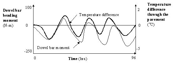
Figure 9. Conceptual schematic of dowel bar bending moment and its correlation to the temperature difference in the slab.

To simulate the effect of wheel loads on the pavement joint, the Falling Weight Deflectometer (FWD) test was used. FWD is one of the most popular nondestructive dynamic testing devices in the pavement industry. The results show, as expected, that the joint did not crack where the strain gages are. Moments in the steel dowel bars were much higher than for the fiberglass bars. Vertical shear in the dowel bars was also calculated at the approach, joint, and leave sections. Again, the vertical shear is greater in the steel dowel bars than in the fiberglass bars.

The addition of a dowel analysis module in HIPERPAV II is feasible. This module could be used to predict the long-term performance of the dowels based on their early-age behavior. If the dowel bearing stress on the concrete is greater than the concrete's bearing strength during the first 72 hours after pavement construction, it is likely that the dowel will loosen from the concrete under additional loading, and its LTE would be reduced. This module could be used to reduce expensive and time-consuming pavement rehabilitation costs, because deterioration of the JCP's transverse joint is one of the most common distresses.

3.4.3 Performance-Related Specifications Study (See references 52, 53, 54, and 55.)

Adding a PRS module to HIPERPAV II for JPCP is a possibility. This section summarizes past work on PRS and describes how a module can be incorporated in HIPERPAV II.

3.4.3.1 Performance-Related Specifications

Acceptance quality characteristics (AQC) are pavement properties that can be measured immediately after construction, such as concrete strength, slab thickness, and initial smoothness, and can be controlled directly by the contractor. PRS is the method that can directly relate these early-age pavement properties directly to pavement performance (distresses), maintenance and rehabilitation (M&R) costs, and finally to the pavement's life cycle costs (LCC). The result of this analysis is the pay adjustment factor for the contractor. Pay adjustment is based on the comparison between the pavement's "As-Designed" LCC (LCC_DES) and the "As-Constructed" LCC (LCC_CON). If LCC_CON is less than LCC_DES because of the high quality of the product delivered by the contractor, then the contractor will receive a pay increase. However, if the opposite occurs, then the contractor will receive a pay decrease. PRS allows for a rational determination of pay adjustment factors. It also can be used to determine the optimal values of the AQC (mean and standard deviation) for the optimal financial return for the contractor and for the State highway agency (SHA). PRS links materials and construction practices directly to pavement performance.

A simplified schematic showing how PRS works is provided in figure 10. PRS are similar to quality assurance (QA) specifications. However, QA specifications only specify the quality of the product and not the desired performance of the pavement. QA specifications address only item 1 in figure 10, while PRS address all 5 items.

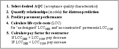
Figure 10. Simple schematic outlining PRS.

First, the SHA should identify the distresses that should be controlled by the specifications. The distresses selected are function of the aspects of pavement performance that the SHA wants to improve.

Second, the desired AQC are selected. These are properties of the pavement that the contractor controls, and are properties that impact the long-term performance of the pavement. At the lowest level of PRS, typical AQC are concrete strength, concrete thickness, air content of the concrete, and initial roughness of the pavement. Other AQC that are being considered for inclusion in the future include percent consolidation around dowels, tie bar depth, and sawcut depth. The mean values and standard deviations of these properties impact the final pay adjustment. Therefore, it is important to adopt an acceptance sampling and testing plan for the determination of these properties. Because the AQC should be obtained immediately after construction, it is necessary to have models that can predict the long-term properties based on the early-age properties.

Third, the pavement distress models are selected. For JPCP, typical distress models selected are indicators of faulting, transverse cracking, transverse spalling, and present serviceability rating (PSR). The models are chosen because they relate the AQC to the distress type. However, AQC are not the only input to these models. In addition, constant values are input to the model, for example climate, traffic, and project location. However, the contractor does not have control over all these properties.

After relating AQC to pavement distresses, pavement performance can be predicted. Figure 11-14 illustrate that PRS quantify the change in the distresses with time.

The fourth step is calculating LCC. LCC takes into account the M&R plan and the unit costs for M&R. M&R costs can be divided into SHA costs and user costs. The SHA costs are day-to-day maintenance, localized rehabilitation (individual slabs and joints), and global rehabilitation (pavement replacement). In the FHWA PaveSpec software, local rehabilitation is considered on a sublot basis and global rehabilitation on a lot basis. Typical costs to the user are travel time, vehicle operation, accident costs, and discomfort costs.

The final step is to calculate pay factors. Different methods are used to calculate pay factors dependent on the level of PRS selected. If a Level A PRS is chosen, then an independent pay factor is calculated for each AQC. Finally, a composite pay factor is calculated which is a mathematical function of each independent AQC. However, if a Level B PRS is selected, the interactions between the AQC are accounted for (e.g., how concrete strength affects pavement thickness). Computer simulation (i.e., using the FHWA PaveSpec software) is necessary to calculate the pay factor.

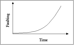
Figure 11. JPCP pavement performance in terms of faulting.

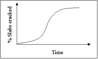
Figure 12. JPCP pavement performance in terms of transverse cracking.

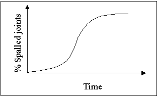
Figure 13. JPCP pavement performance in terms of spalled joints.

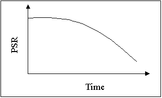
Figure 14. JPCP pavement performance in terms of initial pavement roughness.

3.4.3.2 PRS Benefits

Four benefits of PRS design for SHAs are:^{(52) )}

• PRS provides well-defined AQC target values (mean and standard deviation). A particular pavement quality can be reached if the target AQC is achieved.
• PRS provides a rational means to determine pay adjustments.
• PRS relates construction properties to pavement performance and LCC.
• Pavement costs will decrease once a rational PRS plan has been implemented. This is because both the SHA and the contractor strive to minimize LCC.

3.4.3.3 PRS Levels

There are three discrete levels of PRS implementation.⁽⁵²⁾ Level A is the simplest and most readily implementable PRS. Complexity increases from Level B to Level C. Three factors comprise the PRS levels.

• Methods of acceptance testing (tests currently in use by the SHA).
• Pay adjustment method (with more tests in situ, such as cores, air content, etc.).
• Use of nondestructive tests.

The Level A method of acceptance testing involves in situ sampling and testing from sublots of the constructed concrete pavement. A pavement lot is "a discrete quantity of constructed pavement to which an acceptance procedure (and corresponding pay adjustment) is applied. All pavement placed within a lot should consist of the same mix design and material sources, should be subjected to the same support conditions, and should consist of the same design characteristics."⁽⁵²⁾For Level B, sampling and testing should include additional in situ testing in addition to nondestructive testing. For Level C, nondestructive testing to determine concrete properties primarily should be used. Level C is typically described as a futuristic PRS level.

3.4.3.4 Prospective PRS Module in HIPERPAV II

PRS and HIPERPAV systems can be thought of as truly complementary. PRS are a means to directly address the impacts of various design and construction features on the resulting pavement performance. On the other hand, HIPERPAV is able to verify the impacts that these design and construction features may have with respect to the potential for early-age damage. For example, if strength is selected as an AQC in the PRS system, then the contractor may have an incentive to increase the strength. Often, a higher cement factor is selected to achieve the higher strength. Although the payment under the PRS system could serve to benefit the contractor, the performance may not necessarily improve. Although higher strength will increase the predicted fatigue life of the pavement, the higher cement factor could also lead to early-age problems. The interaction of the advantages and disadvantages of the strength gain are not easy to quantify. The problem is compounded with separate programs (PaveSpec used for PRS, and HIPERPAV used for early-age, damage-related specifications), since the user would need to run both systems independently, requiring manual interpretation from both systems. However, if brought together, the components of the PaveSpec and HIPERPAV predictive capabilities can present the user with this information in a straightforward and easy-to-understand fashion.

To incorporate early-age damage related specification concepts into HIPERPAV, a substantial amount of additional work would have to be performed. As a start point, the lowest equivalent PRS Level A could be added. AQC would have to be designated in the software, and their standard deviations would be included. An additional module would be required so that the lots and sublots could be defined for all sampling and testing. Likewise a pay factor module, an LCC analysis module, and an M&R costs module would need to be added. As new models that are able to predict interactions between concrete properties of interest and innovative test procedures become available, Levels B and C could be incorporated later.

In general, three unique ways of integrating HIPERPAV with standard specifications are possible:

1. Merging standard specifications into HIPERPAV: This method consists of incorporating the text of standard specifications into HIPERPAV through a knowledge base. It would provide recommendations and warnings during the HIPERPAV runs that relate to items considered in the standard specifications, tying them to the inputs in the software.

2. Merging HIPERPAV into standard specifications: In this method, standard specifications could be written to require the use of a temperature management software such as HIPERPAV, further assuring that uncontrolled cracking is avoided.

3. Integrating HIPERPAV and PaveSpec: This method involves combining HIPERPAV and PaveSpec together as described in the above paragraphs, and would be ideal for highway agencies currently considering PRS.

The best option from the above three would depend on the current specifications being used by any individual SHA. It is believed that the first method-merging standard specifications into HIPERPAV-would be the most readily implementable, because it involves less risk to the highway agency in terms of liability. On the other hand, following the current trend of highway agencies shifting to PRS, integrating HIPERPAV and PaveSpec would provide an ideal tool for implementing such a specification.

3.4.4 Curing Study

One FHWA contract currently underway is intended to provide guidelines for curing of PCC pavements (PCCP).⁽⁵⁶⁾ This section describes briefly the objectives of that study, and evaluates the possibility of including the resulting PCCP curing guidelines in HIPERPAV II.

3.4.4.1 PCCP Curing Guidelines

The initial efforts under the FHWA curing study have been compiled into an interim report.⁽⁵⁶⁾ That interim report is the primary source of information in evaluating the guidelines that are expected to be available in the near future.

The primary project objectives identified on the FHWA curing study are:

• Develop a summary of curing standards, current practice, new technologies, and published research.
• Compile gathered information into a guide on curing practices for PCCP.
• Identify deficiencies in the current practice.
• Develop a plan for correcting deficiencies of the current practice.

Based on the information search on PCCP curing, a number of guidelines on curing methods and procedures are recommended in the report. These recommendations are outlined in figure 15. These guidelines primarily address the selection of curing methods, duration of curing, and temperature management during placement.

Selection of Curing Methods. The curing methods section in the guidelines is divided into curing compound methods, water-added methods, and water-retention methods. The selection of curing compounds is primarily based in economic and practical considerations rather than quality or performance.

Selection of the curing compound method is recommended primarily for large placement areas such as highway applications, where the curing compound is the only practical option. Curing compounds are also recommended when other curing materials are unavailable.

Selection of water-added versus water-retention methods is based primarily on the availability of water for hydration. Because water-cement ratios lower than 0.40 lead to insufficient hydration of the cement paste, this threshold is used for selecting curing methods. Water-added methods are recommended whenever the water-cement ratio is equal or less than 0.40, or when expansive cement is used. For water-cement ratios greater than 0.40, the risk of damage to the concrete is lower, and water-retention methods are considered a more viable option. Water-retention methods are also recommended whenever curing compound methods are not suitable, and when no risk on excessive evaporation is present.

For each of the curing methods, additional guidelines on material selection, application rate, time of application, inspection, and curing verification are also presented. The selection is based primarily on select standards, climatic conditions (evaporation rate), mix design and materials (bleeding rate), and recommended practice.

Duration of Curing. Initial guidelines on duration of curing are also presented based on strength-gain rate criteria. However, additional work is required to develop guidelines on the duration of curing based on concrete durability.

Temperature Management. Temperature management is addressed in terms of cold weather concreting and hot weather concreting. For temperature management under hot weather, initial recommendations are made in terms of preventive measures and adjustments to the curing methods (e.g., application rate). Procedures to determine the expected temperature drop in the concrete, and calculation of thermal stresses using software programs such as HIPERPAV, are also considered. In addition, estimating potential risk in concrete strength reduction for high temperature curing is mentioned. Additional work to address this issue is expected. Time of day of construction is also addressed, and recommendations in scheduling construction are made to avoid coincidence of the heat of hydration peak and the maximum temperature of the concrete due to solar radiation.

For temperature management during cold weather, precautions and recommendations are given to protect concrete from freezing, and to maintain a uniform concrete temperature. Primary measures mentioned in the guidelines include: insulation, heated enclosures, and need for moisture retention. More work is expected for developing cold weather concreting guidelines.

3.4.4.2 Benefits of Incorporating the Curing Study in HIPERPAV II

Incorporating the curing guidelines in HIPERPAV II is considered beneficial, as it would complement the software with useful recommendations on improving the performance of concrete pavements through appropriate selection of curing methods, as well as guidelines on the application and duration of curing procedures.

Provided that the curing guidelines address the effect of moisture loss on strength gain, the accuracy of the strength gain prediction with HIPERPAV for different curing methods would also be enhanced.

Finally, it is believed that since HIPERPAV predicts the temperature development in the concrete during the early age, incorporating curing guidelines in HIPERPAV would help users address temperature management-related issues such as thermal stress development, potential of strength reduction (high temperature), strength development during cold weather concreting, and freezing risk.

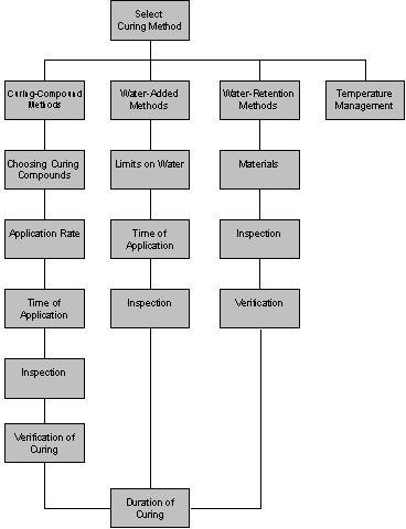
Figure 15. General outline of the FHWA curing guide.⁽⁵⁶⁾

3.4.5 Curling/Warping Study

An FHWA study on the modeling of curling and warping behavior of PCCP (Early and Long-Term Effects of Curling and Warping on Jointed Concrete Pavement-DTFH61-95-C-00021) was under development at the time of writing this report. Although not enough information on the curling/warping study could be obtained at the time of writing this report, the results of this study will include new and improved models for predicting the curling and warping response. Since curling and warping are already an integral part of the HIPERPAV system, these models would be a natural extension to the overall total systems approach in HIPERPAV II.

3.4.6 Mix Optimization Study

Under a research project, "Concrete Mixture Optimization Using Statistical Methods," of the FHWA Concrete Pavement Technology Program (CPTP), a straightforward but powerful approach to select mixture proportions based on a number of performance criteria was developed.^{(57, 58)} The technique had been used previously by the petrochemical and food industries, among others, and was adapted for use on concrete mixes in that project. It employs the use of statistical techniques for optimization of given performance criteria (i.e., slump, strength, cost) based on results from experimental batches. This methodology provides the flexibility for optimizing virtually any combination of performance criteria defined by the user.

Over the past 5 years, FHWA and the National Institute of Standards and Technology (NIST) have further developed this optimization approach, and have recently completed a Web-based application named COST (Concrete Optimization Software Tool).⁽⁵⁹⁾

The mix optimization procedure used in COST is summarized below:

1. Responses to be measured are specified by the user (i.e., slump, strength, cost).

2. The mixture components considered for optimization and proportioning limits for each component are specified.

3. Based on the above information, an experimental design is developed to produce a factorial of mixes for laboratory testing.

4. Trial batches are run and the responses of interests are measured.

5. With the results from laboratory testing, polynomial models are developed and calibrated to predict the performance results as a function of the mix proportions.

6. Weight (desirability) functions are assigned to the various performance measures (i.e., minimum cost, maximum strength, target slump).

7. Statistical tools and plots are used for data analysis and interpretation.

8. Mix designs are scored based on the weight functions assigned for each individual response.

9. Numerical optimization techniques are used to identify optimum mixture proportions.

3.4.6.1 COMET

A simplified concrete mix optimization module named Concrete Optimization, Management, Engineering, and Testing (COMET) is proposed for incorporation in HIPERPAV II. COMET would be based on the same principles used in developing COST. A schematic of COMET is envisioned in figure 16. As seen in this figure, COMET follows the same general logic as previously described, but with some notable modifications. The mix optimization procedure in COMET illustrated in figure 16 is described below:

1. To ensure the greatest potential for implementation (requiring minimal training), mix constituents are limited to cement, pozzolan, water, coarse aggregate, and fine aggregate. Variables that the user can optimize are limited to coarse aggregate fraction, cementitious content, pozzolan substitution, and water-cementitious materials ratio (box 1).

2. Optimization ranges are provided by the user for every variable, and a total of 29 mixes are developed for the experimental program (box 2).

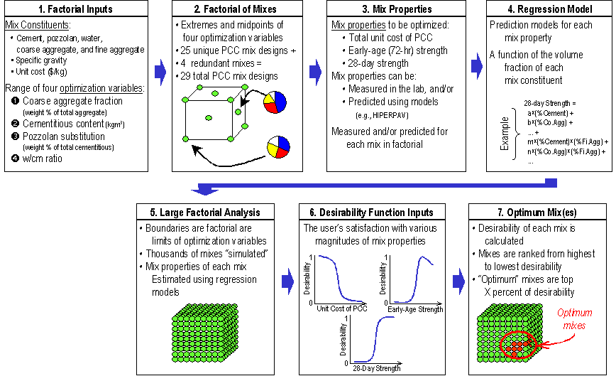
Figure 16. Conceptual representation of the COMET module in HIPERPAV II.

3. Optimization responses are fixed to early-age strength, long-term strength, and cost per cubic yard. A unique addition to the process is made here, whereas the COST system simply prompted the user to enter lab-measured properties. HIPERPAV II optionally utilizes analytical models to predict the same properties. This addition allows the optimization tool to be used in a planning stage, where the mix constituents may not be readily known or available for testing (box 3).

4. Regression models based on the results from the experimental program or from the predicted responses are developed and calibrated to predict the performance results as a function of the mix proportions (box 4).

5. With the models developed, thousands of mixes are simulated, and the responses for every mix computed (box 5).

6. The user has the flexibility to assign desirability functions to the various optimization responses (box 6).

7. Finally, optimum mixes are identified in terms of the individual desirability for every response and in terms of the maximum overall desirability for all responses (box 7).

3.4.7 FHWA Studies Selected for Incorporation

Although all FHWA studies reviewed have a potential for successful implementation in HIPERPAV II, only two of these studies had to be selected. Several factors were considered for this selection, including the status of completion, level of difficulty required for incorporation, easiness of implementation, and usability by the pavement community. Table 15 presents a discussion of the pros and cons considered during the selection process. Based on the advantages and disadvantages identified on each study, the dowel bar study and the mix optimization study were identified as the best candidates for incorporation in HIPERPAV II.

Table 15. Pros and cons of the FHWA studies identified for incorporation in HIPERPAV II.

FHWA Study	Pros	Cons
The Effects of Higher Strength and Associated Concrete Properties on Pavement Performance (FHWA-RD-00-161)(41)	Examines the effect of higher strength and durability properties of concrete on long-term performance and is inline with the objectives of the long-term JPCP module in HIPERPAV II. This study had been completed at the time of this selection.	Although guidelines are provided, no specific models are identified for performance prediction.
Performance of Dowel Bars and Rigid Pavement(51)	Examines the effect of bearing stress at the dowel locations as a result of environmental and traffic loading. Models for prediction of dowel stresses coupled with HIPERPAV predictions are readily available. This study had been completed at the time of this selection.	Simulation of dowel bearing stress for traffic loading may require further development.
Guide to Developing Performance-Related Specifications for PCC Pavements(52 -55)	PRS and HIPERPAV can be used as complimentary tools for identifying desirable acceptance quality characteristics. This study had been completed at the time of this selection.	A substantial amount of additional work would be required for incorporation of this module. Only a small portion of the PRS study could be realistically added within the time constraints for this project.
Curing of Portland Cement Concrete Pavements(56)	This study would complement HIPERPAV with useful recommendations for selection of curing methods. Provided that the curing guidelines address the effect of moisture loss on strength gain, the accuracy of the strength gain prediction with HIPERPAV for different curing methods would be enhanced. The temperature management concepts in the curing guidelines could be complemented with HIPERPAV predictions.	*
Early and Long-Term Effects of Curling and Warping on Jointed Concrete Pavement FHWA contract No. DTFH61-95-C-00021	Models developed for prediction of curling and warping response are directly applicable to HIPERPAV and could be used to enhance prediction of pavement behavior.	*
Concrete Mixture Optimization Using Statistical Methods(57, 58)	The concepts in the mix optimization study are easily implementable in HIPERPAV. Incorporation of this module in HIPERPAV would address the request from many users during previous implementation efforts. This study had been completed at the time of this selection.	No particular drawbacks for incorporating this module in HIPERPAV were noticed.

* At the time of this selection process, this study was still in progress.