• Federal Highway Administration >
• Publications >
• Research Publications >
• 05062 >
• App.Cfm
• Users Manual for LS-DYNA Concrete Material Model 159

Users Manual for LS-DYNA Concrete Material Model 159

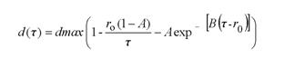
PDF files can be viewed with the Acrobat® Reader®

Appendix A. Modeling Softening

Two formulations the developer has employed to model softening are shown in Figures 108 and 109:

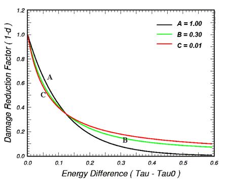
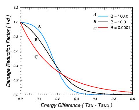
Figure 108. Equation. Old generic damage, small d of τ.

Figure 109. Equation. New generic damage, small d of τ.

The first formulation is the original one used by the developer in older versions of the smooth cap concrete model, as well as the soil model (MAT 147). The second formulation is an updated formulation used by the developer in the concrete model 159 discussed in this report, as well as the wood model (MAT 143).

The equation in Figure 109 has the same number of parameters as the equation in Figure 108, but provides a slightly different fit. Differences in the two softening functions are given in Figure 110 and Figure 111 for dmax = 1. Three different fits are generated for each function. One softening parameter is varied (A or B); the second is held constant (B or A). Note that the updated softening function can model a flat or steep descent upon initiation of damage, whereas the original softening function can only model a steep descent.

Figure 110. Graph. Behavior of the original softening function.

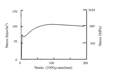
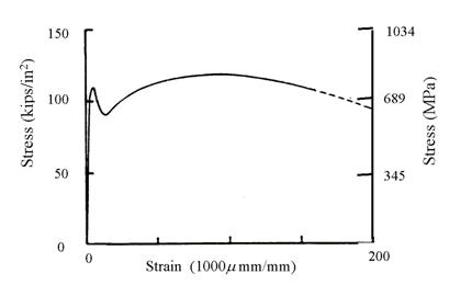
Figure 111. Graph. Behavior of the updated softening function.

Appendix B. Modeling Rebar

Steel is a critical component of reinforced concrete structures, particularly those subjected to dynamic loads. The stress-strain behavior of Grade 60 rebar in tension is shown in Figure 112 and Figure 113 at two strain rates.⁽²⁹⁾ Strain rate affects the initial yield strength more than it does the ultimate yield strength. Rebar behaves in a ductile manner until it breaks at an ultimate strain greater than about 20 percent.

Figure 112. Graph. Rebar yields in a ductile manner at a quasi-static rate of 0.0054/s. Source: U.S. Army Engineer Waterways Experiment Station.⁽²⁹⁾

Figure 113. Graph. Rebar exhibits rate effects at a strain rate of 4/s. Source: U.S. Army Engineer Waterways Experiment Station.⁽²⁹⁾

Rebar is explicitly modeled as beam elements. The properties of the steel are not smeared with those of the concrete. Rebar may be simulated with existing models in LS-DYNA, such as Model #24 (Piecewise Linear Plasticity). The minimum information needed to model rebar is the nominal yield strength.

Typical properties for rebar Model # 24 include:

• Young's modulus E = 200 GPa (29,000 ksi).
• Poisson' Ratio n = 0.3.
• Initial yield strength of 476 MPa (69,037 psi).
• Failure strain of between 13 and 20 percent.
• Tabulated values for yield strength versus plastic strain. These values are extracted from tensile test data like that shown in Figure 113.
• Load curve for rate effects, as shown in Table 11. This table gives the dynamic increase factor versus effective strain rate.

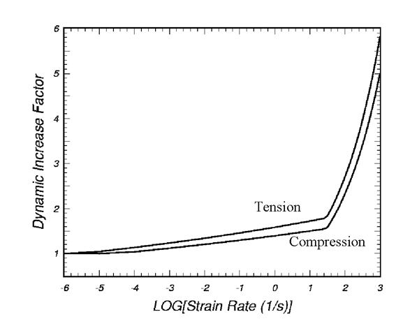
There are two methods of incorporating rebar into the concrete mesh. One is to use common nodes between the rebar and concrete. However, generating a mesh with common nodes may be tedious. A second method is to couple the rebar to the concrete via the CONSTRAINED_LAGRANGE_IN_SOLID command. This formulation couples the slave part (rebar) to the master part (concrete). No information needs to be specified other than the slave and master parts via the *SET_PART_LIST command.

When analyzing reinforced concrete structures, the time step is often controlled by the rebar. If the run time is long due to an excessively small time step, the user may employ a trick to increase the time step when using common nodes. The trick is to connect the rebar beam elements to the concrete hex elements at every other node, instead of every node. This effectively doubles the size of the rebar elements, and therefore doubles the time step. However, some researchers have reported that this may cause unrealistic deformation in the elements in the impact regime. This is because rebar nodes connected to the concrete move less than the unconnected rebar nodes.

Appendix C. Single Element Input File

*KEYWORD

*TITLE

Unconfined Tension of Concrete

$

$$$$$$$$$$$$$$$$$$$$$$$$$$$$$$$$$$$$$$$$$$$$$$$$$$$$$$$$$$$$$$$$$$$$$$$$$$$$$$$$

$

$ Control Output

$

$$$$$$$$$$$$$$$$$$$$$$$$$$$$$$$$$$$$$$$$$$$$$$$$$$$$$$$$$$$$$$$$$$$$$$$$$$$$$$$$

$

*CONTROL_TERMINATION

$ endtim endcyc dtmin endneg endmas

0.60

$

*DATABASE_BINARY_D3PLOT

$ dt

0.001

$

*DATABASE_EXTENT_BINARY

$ neiph neips maxint strflg sigflg epsflg rltflg engflg

1

$ cmpflg ieverp beamip

$

*DATABASE_GLSTAT

$ dt

0.01

$

*DATABASE_MATSUM

$ dt

0.01

$

$$$$$$$$$$$$$$$$$$$$$$$$$$$$$$$$$$$$$$$$$$$$$$$$$$$$$$$$$$$$$$$$$$$$$$$$$$$$$$$$

$

$ Define Parts, Sections, and Materials

$

$$$$$$$$$$$$$$$$$$$$$$$$$$$$$$$$$$$$$$$$$$$$$$$$$$$$$$$$$$$$$$$$$$$$$$$$$$$$$$$$

$...>....1....>....2....>....3....>....4....>....5....>....6....>....7....>....8

$

*PART

$ pid sid mid eosid hgid

Concrete

1 1 159 1

$

*SECTION_SOLID

$ sid elform

1 1

$

*HOURGLASS

$ HGID IHQ QM

1 5 0.01

$

*MAT_CSCM_CONCRETE

$

$ Concrete f'c = 30 MPa Maximum Aggregate Size is 19 mm

$

$ MID RO NPLOT INCRE IRATE ERODE RECOV IRETRC

159 2.320E-09 1 0.0 0 1.05 0.0 0

$

$ PreD

0.0

$

$ f'c Dagg UNITS

30.0 19.0 2

$

$

$$$$$$$$$$$$$$$$$$$$$$$$$$$$$$$$$$$$$$$$$$$$$$$$$$$$$$$$$$$$$$$$$$$$$$$$$$$$$$$$

$

$ Define Nodes and Elements

$

$$$$$$$$$$$$$$$$$$$$$$$$$$$$$$$$$$$$$$$$$$$$$$$$$$$$$$$$$$$$$$$$$$$$$$$$$$$$$$$$

$...>....1....>....2....>....3....>....4....>....5....>....6....>....7....>....8

$

*NODE

$ node x y z tc rc

1 0.000000E+00 0.000000E+00 0.000000E+00 7

2 25.400000000 0.000000E+00 0.000000E+00 5

3 25.400000000 25.40000E+00 0.000000E+00 3

4 0.0000000000 25.40000E+00 0.000000E+00 6

5 0.0000000000 0.000000E+00 25.40000E+00 4

6 25.400000000 0.000000E+00 25.40000E+00 2

7 25.400000000 25.40000E+00 25.40000E+00 0

8 0.0000000000 25.40000E+00 25.40000E+00 1

$

*ELEMENT_SOLID

$ eid pid n1 n2 n3 n4 n5 n6 n7 n8

1 1 1 2 3 4 5 6 7 8

$

$$$$$$$$$$$$$$$$$$$$$$$$$$$$$$$$$$$$$$$$$$$$$$$$$$$$$$$$$$$$$$$$$$$$$$$$$$$$$$$$

$

$ Define Loads

$

$$$$$$$$$$$$$$$$$$$$$$$$$$$$$$$$$$$$$$$$$$$$$$$$$$$$$$$$$$$$$$$$$$$$$$$$$$$$$$$$

$...>....1....>....2....>....3....>....4....>....5....>....6....>....7....>....8

$

*BOUNDARY_PRESCRIBED_MOTION_NODE

$ nid dof vad lcid sf vid

5 3 0 1 1.000E+00

6 3 0 1 1.000E+00

7 3 0 1 1.000E+00

8 3 0 1 1.000E+00

$

*DEFINE_CURVE

$ lcid

1

$ abscissa ordinate

0.000 0.254

500.00000 0.254

$

*END

Appendix D. CEB Specification for Rate Effects

The CEB provides DIFs for both the tensile and compressive strengths in uniaxial stress, as shown in Figures 114 and 115:⁽¹¹⁾

Tensile Strength

Figure 114. Equation. CEB tensile strength dynamic increase factor, DIF _ten.

Here is the effective strain rate (s^-1), which depends on all six strain rate components, and = 30E-06 s^-1.

Compressive Strength

Figure 115. Equation. CEB compressive strength dynamic increase factor, DIF_comp.

The CEB specification is plotted in Figure 116. The specification is valid for strain rates up to about 300 s^-1. Note that DIF is more pronounced in tension than in compression. However, the tensile DIF is not in very good agreement with the tensile data previously reported in Figure 14.

Figure 116. Graph. Dynamic increase factors specified in CEB.

Previous