• Federal Highway Administration >
• Publications >
• Research Publications >
• 05062 >
• Chapt2a.Cfm >
• Users Manual for LS-DYNA Concrete Material Model 159

Users Manual for LS-DYNA Concrete Material Model 159

PDF files can be viewed with the Acrobat® Reader®

Chapter 2. Theoretical Manual

This chapter begins with an overview of concrete behavior, followed by a detailed description of the formulation of concrete material model 159 in LS-DYNA. Equations are provided for each feature of the model (elasticity, plasticity, hardening, damage, and rate effects). The chapter then describes the model input properties and the basis for their default values.

CRITICAL CONCRETE BEHAVIORS

Concrete is a composite material that consists primarily of aggregate and mortar. Its response is complex, ranging from brittle in the tensile and low confining pressure regimes to ductile at high confining pressures. The critical behaviors of concrete are discussed below, particularly those in the tensile and low confining pressure regimes applicable to roadside safety analyses. Figures 1 through 14, which represent these behaviors, are reproduced from the various references cited at the end of each caption.

Stiffness. The elastic behavior of the concrete is isotropic before cracking occurs. This is because the concrete is assumed to be well mixed, vibrated, and not stratified.

Uniaxial Strength. Standard concrete has low tensile strength. The direct pull or unconfined tension strength (f '_T ) is typically 8 to 15 percent of the unconfined compression strength (f '_C ).

Multiaxial Strength. The ultimate strength of concrete depends on both the pressure and shear stresses. Concrete strength data is plotted in Figure 1 and Figure 2 in the meridian and deviatoric planes. Typical failure surfaces that may be fit to such data are represented in Figure 3 and Figure 4. Review of the reference by Chen & Han is highly recommended for a discussion of three-dimensional stress space and the meridian and deviatoric planes.⁽⁷⁾ The general shape of a three-dimensional strength surface can be described by smooth curves in the meridian planes and by its cross-sectional shape in the deviatoric planes.

Concrete strength data is typically plotted as principal stress difference versus pressure. The principal stress difference is σ_x - σ _r. Figure 1 is a nondimensional representation of such a plot. It is well known that concrete fails at lower values of principal stress difference for triaxial extension (TXE) tests than for triaxial compression (TXC) tests conducted at the same pressure. TXC and TXE are standard laboratory tests for measuring failure curves. These tests are typically conducted on cylindrical specimens and begin with hydrostatic compression to a desired confining pressure, i.e., the axial compressive stress, σ_xis equal to the radial compressive stress, σ_r. For TXC tests, the magnitude of the axial compressive stress is quasi-statically increased (holding σ_r constant) until the specimen fails. For TXE tests, the magnitude of the axial compressive stress is quasi-statically decreased until the specimen fails. TXC test data, like that shown in Figure 1, is fit the compressive meridian parameters of the concrete material model.^(8,9) TXE test data is fit to the tensile meridian parameters. This behavior is schematically shown in Figure 3. The shear meridian is obtained from torsion (TOR) tests.

Concrete strength can also be plotted in the deviatoric plane, as shown in Figure 2. Here, nondimensional forms of the principal stresses (σ₁, σ₂, σ₃) are plotted at various nondimensional pressures represented by the solid lines. In the tensile regime, strength data typically form a triangle. In the compressive regime, strength data typically transition from a triangle at low confining pressure to a circle at very high confining pressure. This behavior is schematically shown in Figure 4.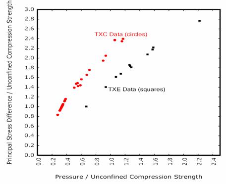

Figure 1. Graph. Example concrete data from Mills and Zimmermann plotted in the meridian plane.⁽⁸⁾

Figure 2. Drawing. Example curves fit by Launay and Gachon to their concrete data and plotted in the deviatoric plane.⁽¹⁰⁾

psi = 145.05 MPa

Figure 3. Graph. Example plots of the failure surfaces of LS-DYNA Model 159 in the meridian plane.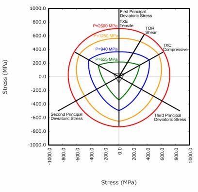

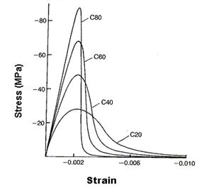
psi = 145.05 MPa

Figure 4. Drawing. Example plots of the failure surfaces of LS-DYNA Model 159 in the deviatoric plane.

Strength Degradation. Concrete softens to near zero strength in the tensile and low confining pressure regimes. This behavior is shown in Figure 5 for a variety of uniaxial strengths.⁽⁹⁾ Concrete also softens at moderate pressures, but the concrete will exhibit a residual strength. This behavior is demonstrated in Figure 6 for concrete tested in TXC at a variety of confining pressures.

psi = 145.05 MPa

Figure 5. Graph. Softening response of concrete in uniaxial compression (reprinted from the Comité Euro-Internacional du Béton (CEB) - Federation for Prestressing (FIP) Model Code 1990, courtesy of the International Federation for Structural Concrete (fib)).⁽¹¹⁾

14 MPa

psi = 145.05 MPa

Stiffness Degradation. As concrete softens, its stiffness also degrades. Consider the cyclic load data shown in Figure 7 through Figure 9 for uniaxial stress in both tension and compression. The unloading occurs along a different slope than the initial loading slope (elastic modulus).

psi = 145.05 MPa

Dilation. Standard concrete exhibits volume expansion under compressive loading at low confining pressures close to pure shear and uniaxial compression. This expansion is called dilation and is as shown in Figure 10 and Figure 11 for uniaxial and biaxial compression data. The volumetric strain decreases initially, because Poisson's ratio is less than 0.5; therefore, the specimens compact in the elastic regime. Dilation initiates just before peak strength (upon initial yield) and continues throughout the softening regime. Concrete does not dilate at high confining pressures greater than about 100 MPa (14,504 psi) (not shown).

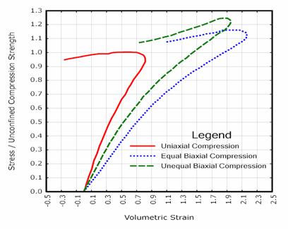Figure 11. Graph. Concrete dilates in biaxial compression.
Source: Data curves scanned from Kupfer et al., American Concrete Institute (ACI).⁽¹⁶⁾

Shear Enhanced Compaction. Concrete hardens due to pore compaction. Consider the pressure-volumetric strain curves schematically shown in Figure 12. This figure demonstrates that the pressure-volumetric strain curve measured in isotropic compression tests is different from that measured in uniaxial strain tests. This difference means that the amount of compaction depends on the amount of shear stress present. This phenomenon is known as shear enhanced compaction. Slight shear enhanced compaction at low confining pressures is expected in roadside safety applications.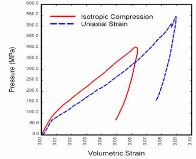

psi = 145.05 MPa

Strain Rate Effects. The strength of concrete increases with increasing strain rate, as shown in Figure 13 and Figure 14. For roadside safety applications, strain rates in the 1 to 10 per second ( /sec) range will produce peak strength increases of about 20 to 50 percent in compression and well more than 100 percent in tension. The initial elastic modulus does not change significantly with strain rate.⁽¹⁷⁾

Overview of Model Theory

This concrete material model was developed to simulate concrete used for the National Cooperative Highway Research Program (NCHRP) 350 roadside safety hardware testing.⁽¹⁹⁾ Performing roadside safety analyses with a finite element code requires a comprehensive material model for concrete, particularly for modeling strain softening in the tensile and low confining pressure regimes. Concrete material model 159 is an enhanced version of the concrete model that the developer has successfully used and progressively developed since 1990 on defense contracts to analyze dynamic loading of reinforced concrete structures. The concrete model is grouped into six formulations for ease of discussion: elastic update, plastic update, yield surface definition, damage, rate effects, and kinematic hardening. Model input parameters used in these formulations, which provide a fit of the model to data, are:

Model control parameters are:

Previous | Table of Contents | Next