• Federal Highway Administration >
• Publications >
• Research Publications >
• 05062 >
• Chapt2b.Cfm >
• Users Manual for LS-DYNA Concrete Material Model 159

Users Manual for LS-DYNA Concrete Material Model 159

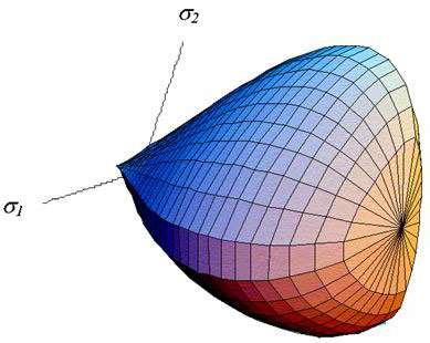
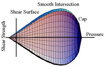
PDF files can be viewed with the Acrobat® Reader®

Chapter 2. Theoretical Manual

Elastic Update

Concrete is typically assumed to be isotropic; therefore, Hooke's Law is used for the elastic stress-strain relationship. Hooke's law depends on two elastic constants: the bulk modulus (K) and the shear modulus (G).

Plastic Update

Following an initial elastic phase, concrete will yield and possibly fail, depending on the state of stress (or type of test being simulated). The yield stresses are defined by a three-dimensional yield surface. The functional form of the yield surface is discussed in the next section. This section briefly discusses the plasticity algorithm responsible for setting the initial yield stresses.

At each time step, the stress is updated from the strain rate increments and the time step via an incremental form of Hooke's Law (an elastic increment). This updated stress is called the trial elastic stress and is denoted σ_ij^T. If the trial elastic stress state lies on or inside the yield surface, the behavior is elastic, and the plasticity algorithm is bypassed. If the trial elastic stress state lies outside the yield surface, the behavior is elastic-plastic (with possible damage, hardening, and rate effects), and the plasticity algorithm returns the stress state to the yield surface. This elastic-plastic stress is called the inviscid stress, and is denoted σ_ij^P.

Details of the return algorithm are well documented.^(20,21) For those knowledgeable about plasticity, the algorithm enforces the plastic consistency condition with associated flow. For efficiency, the algorithm employs subincrementation, rather than iteration, to ensure accurate return of the stress state to the yield surface. Subincrementation is invoked when the current strain increment exceeds a maximum strain limit specified by the user, or defaulted by the model.

The associative return algorithm predicts dilation of the concrete after the yield surface is engaged in the tensile and low confining pressure regimes. Modeling dilation is one reason for employing a sophisticated plasticity algorithm rather than a simple Mises return algorithm. Simple return algorithms do not model dilation.

Yield Surface

The concrete model is a cap model with a smooth or continuous intersection between the failure surface and hardening cap. The general shape of the yield surface in the meridonal plane is shown in Figure 15 and Figure 16. This surface uses a multiplicative formulation to combine the shear (failure) surface with the hardening compaction surface (cap) smoothly and continuously. The smooth intersection eliminates the numerical complexity of treating a compressive 'corner' region between the failure surface and cap. This type of model is often referred to as a smooth cap model or as a continuous surface cap model (CSCM).

Figure 15. Illustration. General shape of the concrete model yield surface in three dimensions.

Figure 16. Illustration. General shape of the concrete model yield surface in two dimensions in the meridonal plane.

The original formulation of the smooth cap model was developed as a function of two stress invariants.⁽²²⁾ The developer extended the formulation to three stress invariants and verified the three-invariant formulation by comparing smooth-cap results with analytical results for the axisymmetric compression of a Mohr-Coulomb medium around a circular hole.^(20,23)

The yield surface is formulated in terms of three stress invariants because an isotropic material has three independent stress invariants. The model uses J_¢-the first invariant of the stress tensor, J′₂-the second invariant of the deviatoric stress tensor, and _J¢3-the third invariant of the deviatoric stress tensor. The invariants are defined in terms of the deviatoric stress tensor, S_ij and pressure, P, as shown in Figure 17:

Figure 17. Equation. Stress invariant J ₁, J′₂, and J′₃.

The three invariant yield function is based on these three invariants, and the cap hardening parameter, κ, as shown in Figure 18:

Figure 18. Equation. Yield function f.

Here F_f is the shear failure surface, F_c is the hardening cap, and ℜ is the Rubin three-invariant reduction factor. Multiplying the cap ellipse function by the shear surface function allows the cap and shear surfaces to take on the same slope at their intersection, as discussed in subsequent paragraphs.

Trial elastic stress invariants are temporarily updated via the trial elastic stress tensor, σ^T. These are denoted J₁^T, J¢₂^T, and J¢₃^T. Elastic stress states are modeled when f (J₁^T, J¢₂^T, J¢₃^T, κ^T) < 0. Elastic-plastic stress states are modeled when f (J₁^T, J¢₂^T, J¢₃^T, κ^T) > 0. In this case, the plasticity algorithm returns the stress state to the yield surface so that f (J₁^P, J¢₂^P, J¢₃^P, κ^P) = 0.

Shear Failure Surface. The strength of concrete is modeled by the shear surface in the tensile and low confining pressure regimes. The shear surface is defined along the compression meridian as shown in Figure 19:

Figure 19. Equation. Shear failure surface function F_f.

Here the values of α, β, l, q are selected by fitting the model surface to strength measurements from TXC tests conducted on plain concrete cylinders (and then adjusting these parameters to account for compaction and damage). The TXC data are typically plotted as principal stress difference versus pressure. The principal stress difference (axial stress minus confining stress) is equal to the square root of 3J¢₂. The shear surface is shown in Figure 20, Figure 21, and Figure 22 for typical concrete values.

psi = 145.05 MPa

Figure 20. Graph. Schematic of shear surface.

psi = 145.05 MPa

Figure 21. Graph. Schematic of two-part cap function.

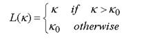
psi = 145.05 MPa

Figure 22. Graph. Schematic of multiplicative formulation of the shear and cap surfaces.

Cap Hardening Surface. The strength of concrete is modeled by a combination of the cap and shear surfaces in the low to high confining pressure regimes. More importantly, the cap is used to model plastic volume change related to pore collapse (although the pores are not explicitly modeled). The initial location of the cap determines the onset of plasticity in isotropic compression and uniaxial strain. The elliptical shape of the cap allows the onset for isotropic compression to be greater than the onset for uniaxial strain, in agreement with shear enhanced compaction data. Without ellipticity, a "flat" cap would produce identical onsets. The motion of the cap determines the shape (hardening) of the pressure-volumetric strain curves via fits with data. Without cap motion, the pressure-volumetric strain curves would be perfectly plastic.

The isotropic hardening cap is a two-part function that is either unity or an ellipse, as shown in Figure 21. When the stress state is in the tensile or very low confining pressure region, the cap function is unity: yield strength via the equation in Figure 18 is independent of the cap. When the stress state is in the low to high confining pressure regimes, the cap function is an ellipse: yield strength depends on both the cap and shear surface formulations. The two-part cap function is defined as shown in Figure 23:

Figure 23. Equation. Cap failure surface function F_c.

where L(κ)is defined as shown in Figure 24:

Figure 24. Equation. L of kappa.

The equation in Figure 23 is equal to unity for J₁ £ L(κ). The equation in Figure 23 describes the ellipse for J₁ > L(κ). The intersection of the shear surface and the cap is at J₁ = κ. κ₀ is the value of J₁ at the initial intersection of the cap and shear surfaces before hardening is engaged (before the cap moves). The equation in Figure 24 restrains the cap from retracting past its initial location at κ₀.

A simpler, but less complete, way of writing the equations in Figure 23 and Figure 24 is shown in Figure 25:

Figure 25. Equation. Simple cap failure surface function F_c.

The intersection of the cap with the J₁ axis is at J₁ = X(κ). This intersection depends on the cap ellipticity ratio R, where R is the ratio of its major to minor axes, as shown in Figure 26:

Figure 26. Equation. X as a function of kappa.

The cap moves to simulate plastic volume change. The cap expands (X(κ) and κ increase) to simulate plastic volume compaction. The cap contracts (X(κ) and κ decrease) to simulate plastic volume expansion, called dilation. The motion (expansion and contraction) of the cap is based on the hardening rule, shown in Figure 27:

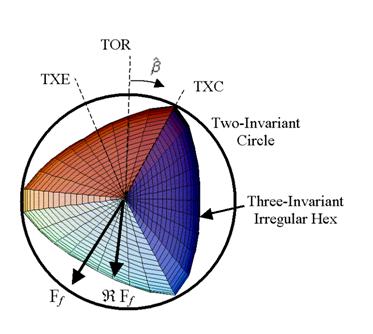
Figure 27. Equation. Plastic volume strain ε ^p_v.

Here ε ^p_v is the plastic volume strain, W is the maximum plastic volume strain, and D₁ and D₂ are model input parameters. X₀ is the initial location of the cap when κ = κ₀.

The five input parameters (X₀, W, D₁, D₂, and R) are obtained from fits to the pressure-volumetric strain curves in isotropic compression and uniaxial strain. X₀ determines the pressure at which compaction initiates in isotropic compression. R, combined with X₀, determines the pressure at which compaction initiates in uniaxial strain. D₁ and D₂ determine the shape of the pressure-volumetric strain curves. W determines the maximum plastic volume compaction.

Rubin Scaling Function. Concrete fails at lower values of J¢₂ (principal stress difference) for TXE and TOR tests than it does for TXC tests conducted at the same pressure. This was previously demonstrated in Figure 1 through Figure 4. This situation indicates that concrete strength depends on the third invariant of the deviatoric stress tensor, J¢₃. When viewed in the deviatoric plane, a three invariant yield surface is triangular or hexagonal in shape, as shown in Figure 28.

The Rubin scaling function ℜ determines the strength of concrete for any state of stress relative to the strength for TXE.^{( 24)} Strengths like TXE and TOR are simulated by scaling back the TXE shear strength by the Rubin function: ℜF_f. The Rubin function ℜ is a scaling function that changes the shape (radius) of the yield surface in the deviatoric plane as a function of angle as shown in Figure 28. This shape may be a circle (Drucker-Prager, Maximum Octahedral Shear Stress, von Mises), a hexagon (Mohr-Coulomb), or an irregular hexagon-like shape (Willam-Warnke) in which each of six sides is quadratic (rather than linear) between the TXC and TXE states.

For comparison, a two-invariant model cannot simultaneously model different strengths in TXC, TXE, and TOR. When viewed in the deviatoric plane, the two-invariant yield surface is a circle, as shown in Figure 28. A two-invariant formulation is modeled with the Rubin function equal to ℜ=1 at all angles around the circle. This means that the TXC, TOR, and TXE strengths are modeled the same.

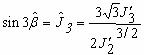
Figure 28. Illustration. Example two- and three-invariant shapes of the concrete model in the deviatoric plane.

The angle is confined to the range -p/6 < < p and is related to the invariants J¢₂ and J¢₃, as shown in Figure 29:

Figure 29. Equation. Angle beta hat in the deviatoric plane.

is a normalized invariant which remains in the range -1 < < 1. For the standard laboratory tests just discussed, the values of and are shown in Figure 30:

Figure 30. Equation. Relationship between beta hat and J hat.

The form of the Rubin scaling function is shown in Figure 31:

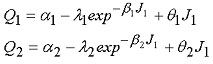
Figure 31. Equation. Rubin scaling function ℜ.

The value of ℜ depends on the state of stress through the angle , and on experimentally determined values (fits to data) for Q₁ and Q₂ as functions of pressure. Strength in TOR is modeled as Q₁F_f. Strength in TXE is modeled as Q₂F_f.

The Rubin three-invariant formulation is implemented because it is more flexible in fitting data than the more commonly used Willam-Warnke formulation. Four example fits of the Rubin formulation are listed below.

1.      Most general fit: the shape of the yield surface in the deviatoric plane transitions with pressure from triangular, to irregular hexagonal, to circular. Input values for all eight parameters: α_λ, l₁, b₁, q₁ and α₂, l₂, b₂, q₂ are shown in Figure 32.

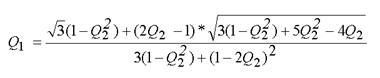
Figure 32. Equation. Most general form for Q₁ and Q₂.

2.     Mohr-Coulomb fit: a straight line fit between the TXE and TXC states. The strength ratios are estimated from the Mohr-Coulomb friction angle ∅ as shown in Figure 33.

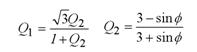
Figure 33. Equation. Mohr-Coulomb form for Q₁, Q₂.

3.     Two-parameter fit: the strength ratios Q₁ and Q₂ remain constant with pressure. Input α₁ and α₂, with all other Rubin parameters set equal to zero. This allows the user to model the yield surface as an irregular (bulging) hexagonal shape in the deviator plane.

4.     Willam-Warnke fit: select Q₂ as a constant or as a function of pressure. Fit Q₁ to the Willam-Warnke TOR surface, as shown in Figure 34.

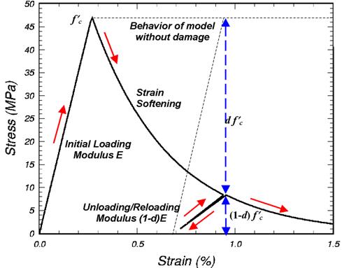
Figure 34. Equation. Willam-Warnke form for Q₁.

Currently, the eight input parameters, which define Q₁ and Q₂, set the shape of the three-invariant yield surface when the pressure is compressive, but not when the pressure is tensile. When the pressure is tensile, the model automatically sets Q₁ = 0.5774 and Q₂ = 0.5. These values simulate a triangular yield surface in the deviatoric plane, and cannot be overridden by the user. With a triangular yield surface, the strengths attained in uniaxial, equal biaxial, and equal triaxial tensile stress simulations are approximately equal.

For a smooth transition between the tensile and compressive pressure regions, the user should take care to set Q₁ = 0.5774 and Q₂ = 0.5 at zero pressure. This is accomplished by setting α₁ - λ₁ = 0.5774 and α₂ - λ₂ = 0.5774.

Damage Formulation

Concrete exhibits softening (strength reduction) in the tensile and low to moderate compressive regimes. Softening is modeled via a damage formulation. Without the damage formulation, the cap model predicts perfectly plastic behavior for laboratory test simulations such as direct pull, unconfined compression, TXE, and TXE. This behavior is not realistic. Although perfectly plastic response is typical of concrete at high confining pressures, it is not representative of concrete at lower confinement and in tension.

The damage formulation models both strain softening and modulus reduction. Strain softening is a decrease in strength during progressive straining after a peak strength value is reached. Modulus reduction is a decrease in the unloading/loading slopes typically observed in cyclic unload/load tests. The damage formulation is based on the work of Simo and Ju, shown in Figure 35.⁽²⁵⁾ Strain softening and modulus reduction are demonstrated in psi = 145.05 MPa

Figure 36 for the concrete model.

Figure 35. Equation. Damaged stress σ ^d_ij.

Here d is a scalar damage parameter that transforms the stress tensor without damage, denoted σ ^vp, into the stress tensor with damage, denoted σ ^d. The damage formation is applied to the stresses after they are updated by the viscoplasticity algorithm. The damage parameter d ranges from zero for no damage to 1 for complete damage. Thus 1 − d is a reduction factor whose value depends on the accumulation of damage. The effect of this reduction factor is to reduce the bulk and shear moduli isotropically (simultaneously and proportionally).

Damage initiates and accumulates when strain-based energy terms exceed the damage threshold. Damage accumulation via the parameter d is based on two distinct formulations, which is called brittle damage and ductile damage.

psi = 145.05 MPa

Figure 36. Graph. This cap model simulation demonstrates strain softening and modulus reduction.

Brittle Damage. Brittle damage accumulates when the pressure is tensile. It does not accumulate when the pressure is compressive. Brittle damage accumulation depends on the maximum principal strain, ε_max, as shown in Figure 37:

Figure 37. Equation. Brittle damage threshold τ_b.

Here τ _b is an energy-type term that depends on the accumulation of total strain via ε_max. Brittle damage initiates when τ _b exceeds an initial threshold r_0b.

Ductile Damage. Ductile damage accumulates when the pressure is compressive. It does not accumulate when the pressure is tensile. Ductile damage accumulation depends on the total strain components, ε_ij, as shown in Figure 38:

Figure 38. Equation. Ductile damage threshold τ_d.

Here τ_d is an energy-type term. The stress components σ_ij are the elasto-plastic stresses (with kinematic hardening) calculated before application of damage and rate effects. Therefore, this strain-energy term does not represent the true strain energy in the concrete. Ductile damage initiates when τ _d exceeds an initial threshold r_0d.

Damage Threshold. Brittle and ductile damage initiate with plasticity. This effectively means that the initial damage surface is coincident with the plastic shear surface. Therefore, a distinct damage surface is not defined by the user. Damage initiates at peak strength on the shear surface where the plastic volume strain is dilative. Damage does not initiate on the cap where plastic volume strain is compactive.

One exception to initiation of damage with initiation of plasticity is when rate effects are modeled via viscoplasticity. With viscoplasticity, the initial damage threshold is shifted (delayed), as shown in Figure 39:

Figure 39. Equation. Viscoplastic damage threshold r₀.

Here r^s is the damage threshold before application of viscoplasticity, and r₀ is the shifted threshold with viscoplasticity. When η is greater than zero (rate effects are modeled), the initial damage threshold is scaled up by the term in brackets. Hence, damage initiation is delayed while plasticity accumulates. This shift requires no input parameters and is hardwired into the model based on the viscoplastic theory previously discussed.

Damage accumulates when either the brittle or ductile energy term, generically called τ_n, exceeds the current damage threshold, r_n. Here the subscript 'n' indicates the nth time step. Once damage initiates, the value of the damage threshold increases. The new threshold at time step n + 1, denoted r_n+1, is set equal to the exceeded value of τ . If the previous value of τ did not exceed the previous threshold (an increment without damage), the threshold does not increase. Mathematically this is expressed as shown in Figure 40:

Figure 40. Equation. Incremental damage threshold, small r_n+1.

Hence each strain energy term (brittle or ductile) must increase in value above its previous maximum in order for damage to accumulate. When energy remains constant or decreases, damage temporarily stops accumulating. The description given here is effectively that of an expanding damage surface.

Softening Function. As damage accumulates, the damage parameter d increases from an initial value of zero, towards a maximum value of 1. Damage accumulates with τ according to the following functions, shown in Figures 41 and 42:

Brittle Damage

Figure 41. Equation. Brittle damage small d of tau.

Ductile Damage

Figure 42. Equation. Ductile damage small d of tau.

An alternative softening function is suggested in appendix A. The parameters A and B or C and D set the shape of the softening curve plotted as stress-displacement or stress-strain. The parameter dmax is the maximum damage level that can be attained. It is set equal to approximately 1 in the tensile and low confining pressure regimes. Brittle damage is set to 0.999 to avoid computational difficulties associated with zero stiffness at a value of 1. At moderate confining pressures, it is less than 0.999, in agreement with TXE data with residual strength. It is set to less than 0.999 by the formula shown in Figure 43:

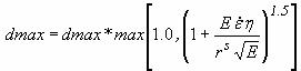
Figure 43. Equation. Variation of dmax with stress invariant ratio.

The power 1.5 was chosen by the developer based on examination of single element simulations and could be included as a user-supplied input parameter at a later date. The maximum damage level also varies with rate effects, as shown in Figure 44. The nondimensional term in parentheses is a stress invariant ratio that is equal to 1 in unconfined compression and less than 1 for stress states with confinement, as shown in Figure 45.

Figure 44. Equation. Variation of dmax with rate effects.

Figure 45. Schematic representation of four stress paths and their stress invariant ratios.

In addition to reducing the maximum damage level with confinement (pressure), the compressive softening parameter, A, may also be reduced with confinement. The formulation is shown in Figure 46:

Figure 46. Equation. Reduction of A with confinement.

Here pmod is a user-specified input parameter. Its default value is 0.0. Input positive value of pmod reduces A when the maximum damage is less than 0.999; otherwise A is unaffected by pmod. Thus, it is only active at moderate confinement levels.

The maximum increment in damage that can accumulate over a single time step is 0.1 (10 percent). This maximum increment is set internally to avoid excessive damage accumulation over a single time step. Excessive damage accumulation can lead to unstable behavior. This 0.1 damage increment was chosen by the developer based on examination of numerous multielement simulations and could be included as a user-supplied input parameter at a later date.

Regulating Mesh Size Sensitivity. If the equations shown in Figure 41 and Figure 42 are used as is to model softening, the softening behavior would be mesh size dependent. This behavior means that different mesh refinements would produce different computational results, typically with the greatest damage accumulation in the smallest elements. This behavior is undesirable and is the result of modeling smaller fracture energy in the smaller elements. The fracture energy is the area under the stress-displacement curve in the softening regime. Direct use of the equations shown in Figure 41 and Figure 42 is demonstrated in the concrete model evaluation report for direct pull and unconfined compression of concrete cylinders.⁽¹⁾ The calculations without softening regulation demonstrate that convergence of the solution is not attained as the mesh is refined to a reasonable element size of about 19 to 38 millimeters (mm) (0.75 to 1.5 inches) for concrete.

It is desirable for a computational solution to converge as the mesh is refined. Regulatory methods promote convergence by reducing or eliminating element-to-element variation in fracture energy. The fracture energy is a property of a material, and special care must be taken to treat it as such. Several possible approaches are available for regulating mesh size dependency. One approach is to manually adjust the damage parameters as a function of element size to keep the fracture energy constant. However, this approach is not practical because the user would need to input different sets of damage parameters for each size element. A more automated approach is to include an element length scale in the model. This is done by passing the element size through to the material model and internally calculating the damage parameters as a function of element size. Finally, viscous methods for modeling rate effects have also been proposed (in the literature) to regulate mesh size dependency. However, if rate-independent calculations are performed, then viscous methods will be ineffective.

To regulate mesh size sensitivity, the concrete model maintains constant fracture energy regardless of element size. This is done by including the element length, L (cube root of the element volume), and a fracture energy type term, G_f , in the softening parameter A of the equation in Figure 41, or C of the equation in Figure 42. The most general way to maintain constant fracture energy is to derive an expression for the fracture energy by integrating the analytical stress-displacement curve as shown in Figure 47:

Figure 47. Equation. Fracture energy integral for G_f.

Here x is the displacement and x₀ is the displacement at peak strength, f¢ . The fracture energy is defined in terms of the damage softening parameters (with dmax = 1) and element length by substituting either damage formulation (equations in Figure 41 or in Figure 42) into and performing the integration. To accomplish the integration, the damage threshold difference (τ - r₀) must be specified. The damage threshold difference is dependent on whether brittle or ductile damage is modeled. Brittle softening (P < 0) and ductile softening (P > 0) are regulated separately, because brittle damage accumulation is modeled differently from ductile damage accumulation.

For brittle damage, the relationship between the fracture energy, G_f, the softening parameters, C and D, the initial damage threshold, r_0b, and element size, L, is shown in Figure 48:

Figure 48. Equation. Brittle damage fracture energy G_f.

This expression was obtained by integrating the equation in Figure 47 using the definition of the damage threshold difference shown in Figure 49:

Figure 49. Equation. Brittle damage threshold difference τ minus small r_0b.

Rearranging the equation in Figure 48 gives the softening parameter C shown in Figure 50:

Figure 50. Equation. Brittle softening parameter C.

For ductile damage, the relationship between the fracture energy, G_f, the softening parameters, A and B, the initial damage threshold, r_0d, and element size, L, is shown in Figure 51:

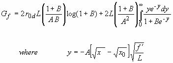
Figure 51. Equation. Ductile damage fracture energy G_f.

This expression was obtained by integrating the equation in Figure 47 using the definition of the damage threshold difference shown in Figure 52:

Figure 52. Equation. Ductile damage threshold difference τ − r_0d.

The integral on the right of the equation in Figure 51 reduces to a dilogarithm, which is not solvable in closed form. Therefore, its value is internally calculated by the LS-DYNA concrete model during the initialization phase. Its value depends on the input parameter B and is termed dilog.

Rearranging the equation in Figure 51 gives the softening parameter A shown in Figure 53:

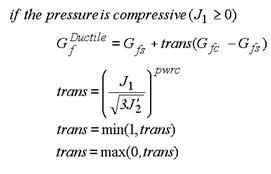
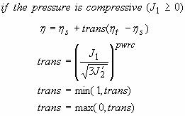
Figure 53. Equation. Ductile softening parameter A.

In summary, to regulate mesh size dependency, the concrete model requires input values for B and G_fc rather than for A and B. Similarly, the concrete model requires input values for D and G_ft rather than for C and D. When the brittle damage threshold is attained, the concrete material model internally solves the equation in Figure 48 for the value of A based on the initial element size, the initial brittle damage threshold, the brittle fracture energy, and a user-specified input value for B. When the ductile damage threshold is attained, the concrete material model internally solves the equation in Figure 51 for the value of C based on the initial element size, the initial ductile damage threshold, and the ductile fracture energy, and a user-specified input value for D.

Refer to the concrete model evaluation report, which discusses cylinder compression calculations conducted with regulation of the softening response.⁽¹⁾ The calculations conducted in tension demonstrate that brittleness increases with mesh refinement until convergence is attained. Conversely, the calculations conducted in compression demonstrate that brittleness decreases with mesh refinement until convergence is attained.

Specifying the Fracture Energy. The user specifies three distinct fracture energy values. These are the fracture energy in uniaxial tensile stress, G_ft, pure shear stress, G_fs, and uniaxial compressive stress, G_fc. The model internally selects the brittle or ductile fracture energy from equations that interpolate between the three fracture energy values as a function of the stress state. The stress state is defined by a nondimensional stress invariant ratio call trans. The interpolation is as shown in Figures 54 and 55:

Figure 54. Equation. Brittle damage threshold G_f ^Brittle.

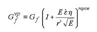
Figure 55. Equation. Ductile damage threshold G_f ^Ductile.

Here trans is the interpolation parameter whose value ranges between 0 in pure shear stress to 1 in uniaxial tensile or compressive stress. The interpolation depends on two user-specified input parameters. These are pwrt for the tensile-to-shear transition and pwrc for the shear-to-compression transition.

Fracture Energy with Rate Effects. When rate effects are modeled with viscoplasticity, the user has the option to increase the fracture energy as a function of the rate effect. This is accomplished via the repow parameter as shown in Figure 56:

Figure 56. Equation. The fracture energy with rate effects, G^vp_f .

Here G_f is either the brittle or ductile fracture energy calculated from the user-specified input values, and is the value that is scaled up with rate effects. A value of repow = 1 is recommended. With a value of 1, the increase in fracture energy with rate effects is approximately proportional to the increase in strength with rate effects. With a value of repow = 0, constant fracture energy is maintained independent of rate effects. Refer to appendix B of the concrete model evaluation report for a review of calculations conducted with repow ranging between 0 and 1.⁽¹⁾ They indicate that repow = 0 tends to model a response that is more brittle than measured in bridge rail impact tests. The recommended range is between 0.5 and 1.

Tracking Damage. Two distinct damage parameters are tracked. One parameter is the ductile damage parameter, denoted d ^d. The ductile damage parameter increases in value whenever the ductile damage formulation is active (pressure is compressive) and τ exceeds the current damage threshold. The value of the ductile damage parameter never decreases, even temporarily.

The other parameter is the brittle damage parameter d ^b. The brittle damage parameter increases in value whenever the brittle (pressure tensile) damage formulation is active and τ exceeds the current damage threshold. When inactive, the brittle damage parameter is temporarily set equal to zero in order to model stiffness recovery with crack closing. In other words, brittle damage drops to zero (stiffness is recovered) whenever the pressure switches from tensile to compressive. The maximum value of d ^b is recovered when the brittle formulation becomes active again (when the pressure becomes tensile again).

A user-specified input parameter, called recov, is available to control stiffness recovery. It is by default zero, which means 100 percent recovery of stiffness and strength when pressure becomes compressive. A value of 1 would provide no recovery of stiffness and strength; hence brittle damage remains at its maximum level. Values between 0 and 1 model partial recovery. Its implementation is shown in Figure 57:

Figure 57. Equation. Default damage recovery of d of τ_t .

The damage parameter applied to the six stresses is equal to the current maximum of the brittle or ductile damage parameter: d=max(d ^b, d ^d).

An option is also available to control stiffness recovery as a function of volumetric strain as well as pressure, as shown in Figure 58:

Figure 58. Equation. Optional damage recovery of d of τ_t.

To select this option, recov is specified by the user with an initial value between 10 and 11, rather than between 0 and 1. When recov is 10 or greater, a flag is internally set to base stiffness recovery on volumetric strain as well as pressure. In addition, the concrete model internally subtracts 10 from recov to obtain a value between 0 and 1 for use in the above formulation.

Element Erosion. An element loses all strength and stiffness as d® 1. To prevent computational difficulties, such as mesh tangling and shooting nodes, element erosion is available as a user option. An element erodes when d > 0.99 and the maximum principal strain is greater than a user-supplied input value.

Rate Effects Formulation

Rate effects formulations are implemented to model an increase in strength with increasing strain rate such as that previously shown in Figure 13. The rate effects formulations are applied to the plasticity surface, the damage surface, and the fracture energy. This section discusses rate effects as they apply to the plasticity surface. Rate effects as they apply to the damage surface and fracture energy were previously discussed in the section on damage formulation above.

Viscoplastic Formulation. The viscoplastic algorithm is applied to the yield surface. The implementation is based on the Simo et al. extension of the commonly used Duvaut-Lions formulation to cap models.⁽²⁶⁾ The Simo et al. extension requires one rate effects parameter, denoted by η. This parameter is called the fluidity coefficient and is a user-specified input parameter.

The basic viscoplastic update algorithm is simple to implement. At each time step, the algorithm interpolates between the elastic trial stress and the inviscid stress (without rate effects) to set the viscoplastic stress (with rate effects), as shown in Figure 59:

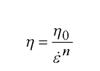
Figure 59. Equation. Viscoplastic stress update for σ^vp_ij.

This interpolation depends on the fluidity coefficient, η, and the time step, Δt. When η = 0, the inviscid stress is attained so that the solution is independent of strain rate. As η ® ¥, the elastic trail stress is attained at each and every time step. This corresponds to the absence of plastic flow. Therefore, plastic flow decreases as rate effects increase. At each time step, the viscoplastic stress is bounded between the current rate-independent stress and the elastic trial stress. The viscoplastic algorithm allows the viscoplastic stress state to lie outside the yield surface.

The model's flexibility in fitting high strain rate data is improved by converting the single parameter viscoplastic formulation to a two-parameter formulation. This is a simple modification, shown in Figure 60, in which:⁽²⁷⁾

Figure 60. Equation. Two-parameter η.

The two input parameters are η₀ and n. The user can fit rate effects data at two strain rates, instead of at one strain rate, which provides a better fit to the data.

The behavior modeled by the viscoplastic update for direct pull and unconfined compression simulations is as shown in Figure 61:

Figure 61. Equation. Dynamic strengths, f ′_T ^dynamic, and f ′_C ^dynamic.

Here it is shown that the dynamic strength (viscoplastic) is equal to the static strength (inviscid) plus a dynamic overstress equal to E η where E is Young's modulus and is the effective strain rate. The effective strain rate depends on all six strain components as shown in Figure 62:

The overstress modeled in tension is the same as that modeled in compression. This means that at high strain rates, the dynamic-to-static strength ratio in tension is about a factor of 10 greater than the dynamic-to-static strength ratio in compression, because the tensile strength is about one-tenth the compressive strength. Hence, the viscoplastic model simulates larger rate effects in tension than in compression, consistent with the data trend previously shown in Figure 14.

Viscoplastic Input. Although the basic two parameter formulation models more significant rate effects in tension than compression, the user may still wish to fit tensile and compressive strain rate data with different viscoplastic fluidity parameters. This is done with four user-specified input parameters. These are η_0t and n_t for fitting uniaxial tensile stress data, and a separate set, η_0c and _c, for fitting the uniaxial compressive stress data.

For stress states between uniaxial tensile stress and uniaxial compressive stress, the fluidity parameter is interpolated as a function of stress invariant ratio. The interpolation is shown in Figures 63 and 64:

Figure 63. Equation. Variation of fluidity parameter η in tension.

Figure 64. Equation. Variation of fluidity parameter η in compression.

Here, the effective η_t , η_s , and η_c are the fluidity parameters in uniaxial tensile stress, shear stress, and uniaxial compressive stress. They are determined from five input parameters as shown in Figure 65:

Figure 65. Equation. Effective fluidity parameters, η_t, η_c, and η _s.

The effective fluidity parameter in shear is determined from a single input scaling parameter, Srate.

This viscoplastic model may predict substantial rate effects at high strain rates ( > 100). To limit rate effects at high strain rates, the user may input overstress limits in tension (overt) and compression (overc). These input parameters limit calculation of the fluidity parameter as shown in Figure 66:

Figure 66. Equation. Overstress limit of η.

where over = overt when the pressure is tensile, and over = overc when the pressure is compressive.

Kinematic Hardening

In unconfined compression, the stress-strain behavior of concrete typically exhibits nonlinearity and dilation prior to the peak. This behavior was previously demonstrated in Figure 5 and Figure 10. This type of behavior is modeled with an initial shear yield surface, N_HF_f , which hardens until it coincides with the ultimate shear yield surface, F_f. Two input parameters are required. One parameter, N_H, initiates hardening by setting the location of the initial yield surface as a fraction of the final yield surface. Reasonable values are approximately 0.7 < N_H £ 1.0. A second parameter, C_H, determines the rate of hardening (amount of nonlinearity).

Figure 67. Equation. Back stress α _ij ^{n + 1}.

Figure 68. Equation. Updated stress with hardening, σ^P _ij ⁿ⁺¹.

The hardening rule defines the growth of the back stress. Hardening rules are typically based on stress or plastic strain. The model bases hardening upon stress to ensure that the translating shear surface coincides with the ultimate surface (lack of proper translation is a problem with plastic strain based rules). This process is accomplished by defining the incremental back stress, as shown in Figure 69:

Figure 69. Equation. Incremental back stress, Δα_ij.

Here C_H is the user input parameter that determines the rate of translation, G_α is a function that properly limits the increments, and - α_ij are the elastoplastic stress components that determines the direction of translation for each component. Also included in the formulation is the effective strain rate increment, , and the time step, Δt. These terms are internally calculated by the material model and LS-DYNA, and are included to keep the hardening response independent of time step, time step scale factor, and strain increment.

The input parameter C_H is the rate of translation used in unconfined compression. In the brittle regime (and for pure shear stress) the rate of translation is internally increased to 10C_H. For stress states with low confinement, the rate of translation transitions between the brittle value and the input value are shown in Figures 70 and 71:

Figure 70. Equation. Brittle rate of translation C_H ^Brittle.

Figure 71. Equation. Ductile rate of translation C_H ^Ductile.

The function G_α restricts the motion of the yield surface so that it cannot translate outside the ultimate surface.⁽²³⁾ The functional form of G_α is determined from the functional form of the yield surface. It is defined as shown in Figure 72:

Figure 72. Equation. The limiting function G_α.

The value of the limiting function is G_α = 1 at initial yield, because α_ij = 0 at initial yield. The value of the limiting function is G_α = 0 at ultimate yield, because the numerator equals the denominator (for the main term in brackets) at ultimate yield. Thus, G_α limits the growth of the back stress as the ultimate yield surface is approached. The developer has chosen to square the term in brackets based on review of the behavior of single element simulations. The square power could be replaced with a user-defined input parameter at a later date.

Each term in the denominator warrants a verbal description. The term on the left is the value of the ultimate yield surface, evaluated at the pressure invariant with backstress (before application of damage and viscoplasticity). The term on the right is the value of the initial yield surface, evaluated at the pressure invariant without backstress (also before application of damage and viscoplasticity).

Use of the kinematic hardening formulation modifies the shear surface definition, as shown in Figure 73:

Figure 73. Equation. Modified shear failure surface, F_f.

If kinematic hardening is not requested (C_H and N_H are set to zero), then the value of N_H is internally reset to 1.0. In this way, the original (ultimate) shear surface is recovered.

Model Input

Ease of use is an important consideration for the roadside safety community. Many users have significant experience performing LS-DYNA analyses, but they are less experienced in material modeling topics. Often, users lack the necessary time, data, and material modeling experience to accurately fit a set of material model parameters to data. The ability of a material model to simulate real world behavior not only depends on the theory of the material model, but on the fit of the material model to laboratory test data. The current version of concrete material model 159 has up to 37 input parameters, with a minimum of 19 parameters that must be fit to data. The model has been made easy to use by implementing a set of standardized material properties for use as default material properties.

Default material model parameters are provided for the concrete model based on three input specifications: the unconfined compression strength (grade), the aggregate size, and the units. The parameters are fit to data for unconfined compression strengths between about 20 and 58 MPa (2,901 to 8,412 psi), with emphasis on the midrange between 28 and 48 MPa (4,061 and 6,962 psi). The unconfined compression strength affects all aspects of the fit, including stiffness, three-dimensional yield strength, hardening, and damage. The fracture energy affects only the softening behavior of the damage formulation. Softening is fit to data for aggregate sizes between 8 and 32 mm (0.3 and 1.3 inches).

The suite of material properties was primarily obtained through use of the CEB-FIP Model Code.⁽¹¹⁾ This code is a synthesis of research findings and contains a thorough section on concrete classification and constitutive relations. Various material properties, such as compressive and tensile strengths, stiffness, and fracture energy, are reported as a function of grade and aggregate size.

Previous | Table of Contents | Next