U.S. Department of Transportation
Federal Highway Administration
1200 New Jersey Avenue, SE
Washington, DC 20590
202-366-4000


Skip to content
Facebook iconYouTube iconTwitter iconFlickr iconLinkedInInstagram

Federal Highway Administration Research and Technology
Coordinating, Developing, and Delivering Highway Transportation Innovations

Report
This report is an archived publication and may contain dated technical, contact, and link information
Publication Number: FHWA-HRT-05-062
Date: May 2007

Users Manual for LS-DYNA Concrete Material Model 159

PDF Version (1.49 KB)

PDF files can be viewed with the Acrobat® Reader®

Chapter 3. Users Manual

This chapter is intended to be a brief Users Manual for those who want to run the model with a cursory, rather than indepth, understanding of the underlying theory and equations. This chapter begins with a description of the LS-DYNA concrete model input, followed by a brief theoretical description of the model theory. All information in this chapter is included in the LS-DYNA Keyword Users Manual.(6)

LS-DYNA Input

*MAT_CSCM {OPTION}

This is material type 159. This is a smooth or continuous surface cap model and is available for solid elements in LS-DYNA. The user has the option of inputting his or her own material properties (<BLANK> option), or requesting default material properties for normal strength concrete (CONCRETE).

Options include:

<BLANK>

CONCRETE

In selecting an option the keyword cards appear:

*MAT_CSCM

*MAT_CSCM _CONCRETE

Define the following card for all options.

Card Format

Card 1

1

2

3

4

5

6

7

8

Variable

MID

RO

NPLOT

INCRE

IRATE

ERODE

RECOV

IRETRC

Type

I

F

I

F

I

F

F

F


Card 2

1

2

3

4

5

6

7

8

Variable

PreD


Type

F


Define the following card for the CONCRETE option. Do not define for the <BLANK> option.

Card 2

1

2

3

4

5

6

7

8

Variable

f 'C

Dagg

UNITS

         
Type

F

F

I


Define the following cards for the <BLANK> option. Do not define for CONCRETE.

Card 3

1

2

3

4

5

6

7

8

Variable

G

K

α

θ

λ

β

NH

CH

Type

F

F

F

F

F

F

F

F


Card 4

1

2

3

4

5

6

7

8

Variable

αλ

θλ

λλ

βλ

α2

θ2

λ2

β2

Type

F

F

F

F

F

F

F

F


Card 5

1

2

3

4

5

6

7

8

Variable

R

X0

W

D1

D2


Type

F

F

F

F

F


Card 6

1

2

3

4

5

6

7

8

Variable

B

Gfc

D

Gft

Gfs

pwrc

pwrt

pmod

Type

F

F

F

F

F

F

F

F


Card 7

1

2

3

4

5

6

7

8

Variable

η0c

Nc

η0t

Nt

overc

overt

Srate

repow

Type

F

F

F

F

F

F

F

F

Define for all options.

Variable
Description
MID Material identification. A unique number must be chosen.
RO  Mass density.
NPLOT Plotting options:
  • EQ. 1.    Maximum of brittle and ductile damage (default).
  • EQ. 2     Maximum of brittle and ductile damage, with recovery of brittle damage.
  • EQ. 3.    Brittle damage.
  • EQ. 4.    Ductile damage.
  • EQ. 5.    k (intersection of cap with shear surface).
  • EQ. 6.    X0 (intersection of cap with pressure axis).
  • EQ. 7.   Epsilon superscript rho subscript nu (plastic volume strain).
INCRE Maximum strain increment for subincrementation. If left blank, a default value is set during initialization based upon the shear strength and stiffness.
IRATE Rate effects options:
  • EQ.  0. Rate effects model turned off (default).
  • EQ.  1. Rate effects model turned on.
ERODE Elements erode when damage exceeds 0.99 and the maximum principal strain exceeds 1-ERODE. For erosion that is independent of strain, set ERODE equal to 1.0. Erosion does not occur if ERODE is less than 1.0.
RECOV The modulus is recovered in compression when RECOV is equal to 0 (default). The modulus remains at the brittle damage level when RECOV is equal to 1. Partial recovery is modeled for values of RECOV between 0 and 1.
IRETRC Cap retraction option:
  • EQ. 0. Cap does not retract (default).
  • EQ. 1. Cap retracts.
PreD Preexisting damage (0 £ PreD < 1). If left blank, the default is zero (no preexisiting damage).


Define for CONCRETE option.

Variable Description
f 'C Unconfined compression strength. If left blank, default is 30 MPa (4,351 psi).
Dagg Maximum aggregate size. If left blank, default is 19 mm (0.75 inch).
UNITS

Units options:

  • EQ. 0. GPa, mm, milliseconds, kg/mm3, kN
  • EQ. 1. MPa, mm, milliseconds, g/mm3, N
  • EQ. 2. MPa, mm, seconds, mg/mm3, N
  • EQ. 3. psi, inch, seconds, lb-s2/inch4, lb
  • EQ. 4. Pa, m, seconds, kg/m3, N

Remarks:

Default concrete input parameters are for normal strength concrete with unconfined compression strengths between about 20 and 58 MPa (2,901 and 8,412 psi).

Define for <BLANK> option only.
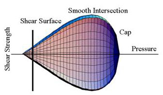
Variable Description 
G shear modulus
K bulk modulus
α TXE surface constant term
θ TXC surface linear term
λ TXC surface nonlinear term
β TXC surface exponent
α1  TOR surface constant term
θ1 TOR surface linear term
λλ TOR surface nonlinear term
βλ  TOR surface exponent
α2 TXE surface constant term
θ2  TXE surface linear term
λ2 TXE surface nonlinear term
β2 TXE surface exponent
NH hardening initiation
CH hardening rate
R cap aspect ratio
X0 cap initial location
W maximum plastic volume compaction
D1 linear shape parameter
D2 quadratic shape parameter
B ductile shape softening parameter
Gfc fracture energy in uniaxial stress
D Brittle shape softening parameter
Gft fracture energy in uniaxial tension
Gfs fracture energy in pure shear stress
pwrc shear-to-compression transition parameter
pwrt shear-to-tension transition parameter
pmod modify moderate pressure softening parameter
η0c rate effects parameter for uniaxial compressive stress
Nc rate effects power for uniaxial compressive stress
η0t rate effects parameter for uniaxial tensile stress
Nt rate effects power for uniaxial tensile stress
overc maximum overstress allowed in compression
overt maximum overstress allowed in tension
Srate ratio of effective shear stress to tensile stress fluidity parameters
repow power that increases fracture energy with rate effects

Model Formulation and Input Parameters

This is a cap model with a smooth intersection between the shear yield surface and hardening cap, as shown in Figure 84. The initial damage surface coincides with the yield surface. Rate effects are modeled with viscoplasticity.

Figure 84. Graph. General shape of the concrete model yield surface in two dimensions.

Figure 84. Illustration. General shape of the concrete model yield surface in two dimensions.

Stress Invariants. The yield surface is formulated in terms of three stress invariants: J1, the first invariant of the stress tensor; J¢2, the second invariant of the deviatoric stress tensor; and J¢3, the third invariant of the deviatoric stress tensor. The invariants are defined in terms of the deviatoric stress tensor, Sij and pressure, P, as shown in Figure 85:

Figure 85. Equation. Three stress invariants, J subscript 1, J prime subscript 2, and J prime subscript 3. J subscript 1 equals three times P. J prime subscript 2 equals one-half times the deviatoric stress S subscript lowercase IJ times the deviatoric stress S subscript lowercase IJ. J prime subscript 3 equals one-third times the deviatoric stress S subscript lowercase IJ times deviatoric stress S subscript lowercase JK times deviatoric stress S subscript lowercase KI.

Figure 85. Equation. Three stress invariants, J1, J2, J3.

Plasticity Surface. The three invariant yield function is based on these three invariants, and the cap hardening parameter, κ, as shown in Figure 86:

Figure 86. Equation. Plasticity yield function lowercase F. Yield surface lowercase F as a function of J subscript 1, J prime subscript 2, J prime subscript 3, and kappa equals J prime subscript 2 minus the quantity of the Rubin function R superscript 2, times the shear failure surface function F subscript lowercase F superscript 2, times the cap failure surface function F subscript lowercase C.

Figure 86. Equation. Plasticity yield function f.

Here Ff is the shear failure surface, Fc is the hardening cap, and ℜ is the Rubin three-invariant reduction factor. The cap hardening parameter κ is the value of the pressure invariant at the intersection of the cap and shear surfaces.

Trial elastic stress invariants are temporarily updated via the trial elastic stress tensor, σT. These are denoted J1T, J¢2T, and J¢3T. Elastic stress states are modeled when f (J1T, J¢2T, J¢3T, κT ) < 0. Elastic-plastic stress states are modeled when f (J1T, J¢2T, J¢3T, κT ) > 0. In this case, the plasticity algorithm returns the stress state to the yield surface in a manner that f (J1P, J¢2P, J¢3P, κP) = 0.

Shear Failure Surface. The strength of concrete is modeled by the shear surface in the tensile and low confining pressure regimes (see Figure 87):

Figure 87. Equation. Shear failure surface function F subscript lowercase F. Shear failure surface F subscript lowercase F as a function of J subscript 1 equals alpha, minus the quantity lambda times the exponential function of minus beta times J subscript 1, plus the quantity theta times J subscript 1.

Figure 87. Equation. Shear surface function Ff.

Here the values of Alpha, Beta, Lambda and Theta are selected by fitting the model surface to strength measurements from TXC tests conducted on plain concrete cylinders.

Rubin Scaling Function. Concrete fails at lower values of 2(principal stress difference) for TXE and TOR tests than it does for TXC tests conducted at the same pressure. The Rubin scaling function ℜ determines the strength of concrete for any state of stress relative to the strength for TXE, via ℜFf. Strength in TOR is modeled as Q1Ff . Strength in TXE is modeled as Q2Ff, in Figure 88, where:

Figure 88. Equation. Most general form for scaling functions Q subscript 1, Q subscript 2. Q subscript 1 equals alpha subscript 1 minus lambda subscript 1 times the exponential of negative beta subscript 1 times J subscript 1, all plus theta times J subscript 1. Q subscript 2 equals alpha subscript 2 minus lambda subscript 2 times the exponential of negative beta subscript 2 times J subscript 1, all plus theta subscript 2 times J subscript 1.

Figure 88. Equation. Most general form for scaling functions Q1, Q2.

Cap Hardening Surface. The strength of concrete is modeled by a combination of the cap and shear surfaces in the low to high confining pressure regimes. The cap is used to model plastic volume change related to pore collapse (although the pores are not explicitly modeled). The isotropic hardening cap is a two-part function that is either unity or an ellipse, as shown in Figure 89:

Figure 89. Equation. Cap surface function, F subscript lowercase C. Cap failure surface F subscript lowercase C as a function of J subscript 1 and kappa, equals 1 minus the quantity of a numeration divided by a denominator. The numerator is the multiplication of 2 quantities. The first quantity is J subscript 1 minus L of kappa. The second quantity is the absolute value of J subscript 1 minus L of kappa all added to J subscript 1 minus L of kappa. The numerator is 2 times the quantity of X of kappa minus L of kappa, superscript 2.

Figure 89. Equation. Cap surface function, Fc.

where L(κ) is defined in Figure 90:

Figure 90. Equation. Definition of L of kappa. L of kappa equals one of two values. The value is kappa if kappa is greater than kappa subscript 0. The value is kappa subscript 0 otherwise.

Figure 90. Equation. Definition of L of kappa.

The equation for Fc is equal to unity for J1 £ L(κ). It describes the ellipse for J1 > L(κ). The intersection of the shear surface and the cap is at J1 = κ. κ0 is the value of J1 at the initial intersection of the cap and shear surfaces before hardening is engaged (before the cap moves). The equation for L(κ) restrains the cap from retracting past its initial location at κ0.

The intersection of the cap with the J1 axis is at J1 = X(κ). This intersection depends on the cap ellipticity ratio R, where R is the ratio of its major to minor axes (see Figure 91):

Figure 91. Equation. Pressure invariant X as a function of kappa. X as a function of kappa equals L of kappa plus the cap aspect ratio R times the shear surface function F subscript lowercase F as a function of L of kappa.

Figure 91. Equation. Pressure invariant X as a function of kappa.

The cap moves to simulate plastic volume change. The cap expands (X(κ) and κincrease) to simulate plastic volume compaction. The cap contracts (X(κ) and κ decrease) to simulate plastic volume expansion, called dilation. The motion (expansion and contraction) of the cap is based on the hardening rule, as shown in Figure 92:

Figure 92. Equation. Plastic volume strain hardening rule, epsilon superscript lowercase P subscript lowercase V. Epsilon superscript lowercase P subscript lowercase V equals the maximum plastic volume strain W times the quantity of one minus exponential to a power. The power is minus D subscript 1 times the quantity X minus X subscript 0, minus D subscript 2 times the quantity squared of X minus X subscript.

Figure 92. Equation. Plastic volume strain hardening rule, ε pv.

Here ε ρv is the plastic volume strain, W is the maximum plastic volume strain, and D1 and D2 are model input parameters. X0 is the initial location of the cap when κ= κ0.

The five input parameters (X0, W, D1, D2, and R) are obtained from fits to the pressure-volumetric strain curves in isotropic compression and uniaxial strain. X0 determines the pressure at which compaction initiates in isotropic compression. R, combined with X0, determines the pressure at which compaction initiates in uniaxial strain. D1 and D2 determine the shape of the pressure-volumetric strain curves. W determines the maximum plastic volume compaction.

Shear Hardening Surface. In unconfined compression, the stress-strain behavior of concrete exhibits nonlinearity and dilation before the peak. This type of behavior is modeled with an initial shear yield surface, NHFf, which hardens until it coincides with the ultimate shear yield surface, Ff. Two input parameters are required. One parameter, NH, initiates hardening by setting the location of the initial yield surface. A second parameter, CH, determines the rate of hardening (amount of nonlinearity).

Damage. Concrete exhibits softening in the tensile and low to moderate compressive regimes (see Figure 93):

Figure 93. Equation. Transformation of viscoplasticstress to damaged stress, sigma subscript lowercase IJ superscript lowercase D. Sigma subscript lowercase IJ superscript lowercase D equals sigma subscript lowercase IJ superscript lowercase VP times the quantity 1 minus lowercase D.

Figure 93. Equation. Transformation of viscoplastic stress to damaged stress, σdij.

A scalar damage parameter, d, transforms the viscoplastic stress tensor without damage, denoted s vp, into the stress tensor with damage, denoted s d. Damage accumulation is based on two distinct formulations, which are called brittle damage and ductile damage. The initial damage threshold is coincident with the shear plasticity surface; thus, the user does not have to specify the threshold.

Ductile Damage. Ductile damage accumulates when the pressure (P) is compressive and an energy-type term, τd, exceeds the damage threshold, r0d. Ductile damage accumulation depends on the total strain components, εij, as shown in Figure 94:

Figure 94. Equation. Ductile damage accumulation, tau subscript lowercase D. Tau subscript lowercase D equals the square root of the quantity one-half times the sigma subscript lowercase IJ times epsilon subscript lowercase IJ.

Figure 94. Equation. Ductile damage accumulation, τ d.

The stress components sij are the elasto-plastic stresses (with kinematic hardening) calculated before application of damage and rate effects.

Brittle Damage. Brittle damage accumulates when the pressure is tensile and an energy-type term, τb, exceeds the damage threshold, r0b. Brittle damage accumulation depends on the maximum principal strain, εmax, as shown in Figure 95:

Figure 95. Equation. Brittle damage accumulation, tau subscript b. Tau subscript lowercase B equals the square root of the quantity E times the square of epsilon subscript max.

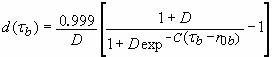
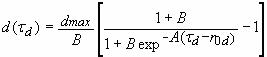
Figure 95. Equation. Brittle damage accumulation, τb.

Softening Function. As damage accumulates, the damage parameter d increases from an initial value of zero, towards a maximum value of 1, via Figures 96 and 97:

Figure 96. Equation. Brittle damage, lowercase D of tau subscript lowercase B. Lowercase D of tau subscript lowercase B equals 0.999 divided by D times a numerator divided by a denominator minus 1. The numerator is 1 plus D. The denominator is 1 plus D times the exponential of negative C times left parenthesis tau subscript lowercase T minus tau subscript 0 and lowercase T right parenthesis.

Figure 96. Equation. Brittle damage, d of tb.

Figure 97. Equation. Ductile damage, lowercase D of tau subscript lowercase D. Lowercase D of tau subscript lowercase C equals dmax divided by B times a numerator divided by a denominator minus 1. The numerator is 1 plus B. The denominator is 1 plus B times the exponential of negative A times left parenthesis tau subscript lowercase C minus tau subscript 0 and lowercase C right parenthesis.

Figure 97 Equation. Ductile damage, d of τd.

The damage parameter applied to the six stresses is equal to the current maximum of the brittle or ductile damage parameter. The parameters A and B or C and D set the shape of the softening curve plotted as stress-displacement or stress-strain. The parameter dmax is the maximum damage level that can be attained. It is calculated internally and is less than 1 at moderate confining pressures. The compressive softening parameter, A, may also be reduced with confinement, using the input parameter pmod, as shown in Figure 98:

Figure 98. Equation. Reduction of A with confinement. A equals A times left parenthesis dmax plus 0.001 right parenthesis superscript pmod.

Figure 98. Equation. Reduction of A with confinement.

Regulating Mesh Size Sensitivity. The concrete model maintains constant fracture energy, regardless of element size. The fracture energy is defined here as the area under the stress-displacement curve from peak strength to zero strength. Constant fracture energy is achieved by internally formulating the softening parameters A and C in terms of the element length, L (cube root of the element volume), the fracture energy, Gf, the initial damage threshold, τ0t or τ0c , and the softening shape parameters, D or B.

The fracture energy is calculated from up to five user-specified input parameters (Gfc, Gft, Gfs, pwrc, pwrc). The user specifies three distinct fracture energy values. These are the fracture energy in uniaxial tensile stress, Gft, pure shear stress, Gfs, and uniaxial compressive stress, Gfc. The model internally selects the fracture energy from equations, which interpolate between the three fracture energy values as a function of the stress state (expressed via two stress invariants). The interpolation equations depend on the user-specified input powers pwrc and pwrt, as shown in Figure 99:

Figure 99. Equation. Brittle and ductile damage thresholds, G subscript lowercase F. If the pressure is tensile, meaning J subscript 1 is less than 0, then G subscript lowercase F equals G subscript lowercase F and lowercase S plus parameter trans times the difference between G subscript lowercase FT and G subscript lowercase FS, where parameter trans equals the negative J subscript 1 divided by the square root of the quantity 3 times J prime subscript 2, all to the power of parameter pwrt. If the pressure is compressive, meaning J subscript 1 is greater than or equal to 0, then G subscript lowercase F equals G subscript lowercase F and lowercase S plus parameter trans times the difference between G subscript lowercase FC and G subscript lowercase FS, where parameter trans equals the positive J subscript 1 divided by the square root of the quantity 3 times J prime subscript 2, all to the power of parameter pwrc.

Figure 99. Equation. Brittle and ductile damage thresholds, Gf.

The internal parameter trans is limited to range between 0 and 1.

Element Erosion. An element loses all strength and stiffness as d®1. To prevent computational difficulties with very low stiffness, element erosion is available as a user option. An element erodes when d > 0.99 and the maximum principal strain is greater than a user-supplied input value, 1-ERODE.

Viscoplastic Rate Effects. At each time step, the viscoplastic algorithm interpolates between the elastic trial stress, Sigma superscript tau subscript lowercase i j, and the inviscid stress (without rate effects), Sigma superscript rho subscript lowercase i j , to set the viscoplastic stress (with rate effects), :Sigma superscript lowercase v p subscrip lowercase i j as shown in Figure 100:

Figure 100. Equation. Viscoplastic stress, sigma subscript lowercase IJ superscript lowercase VP. Sigma subscript lowercase IJ superscript lowercase VP equals the quantity 1 minus gamma, times sigma subscript lowercase IJ superscript T plus gamma times sigma subscript lowercase IJ superscript P, where gamma equals delta lowercase T divided by eta, divided by the quantity of 1 plus delta lowercase T divided by eta.

Figure 100. Equation. Viscoplastic stress, σvpij.

This interpolation depends on the effective fluidity coefficient, η, and the time step, Δt. The effective fluidity coefficient is internally calculated from five user-supplied input parameters and interpolation equations shown in Figure 101:

Figure 101. Equation. Variation of fluidity parameter eta in tension and compression. If the pressure is tensile, meaning J subscript 1 is less than 0, then eta equals eta subscript lowercase S plus parameter trans times the difference between eta subscript lowercase T and eta subscript lowercase S, where parameter trans equals the negative J subscript 1 divided by the square root of the quantity 3 times J prime subscript 2, all to the power of parameter pwrt. If the pressure is compressive, meaning J subscript 1 is less than 0, then eta equals eta subscript lowercase S plus parameter trans times the difference between eta subscript lowercase C and eta subscript lowercase S, where parameter trans equals the positive J subscript 1 divided by the square root of the quantity 3 times J prime subscript 2, all to the power of parameter pwrc. Here, Eta subscript lowercase T equals eta subscript 0 lowercase T, divided by dot epsilon to the power of lowercase N subscript lowercase T. Eta subscript lowercase C equals eta subscript 0 lowercase C, divided by dot epsilon to the power of lowercase N subscript lowercase C. Eta subscript lowercase S equals parameter Srate times eta subscript lowercase T.

Figure 101. Equation. Variation of the fluidity parameter η in tension and compression.

The input parameters are η0t and Nt for fitting uniaxial tensile stress data, η0c and Nc for fitting the uniaxial compressive stress data, and Srate for fitting shear stress data. The effective strain rate is shown in Figure 102:

Figure 102. Equation. Definition of effective strain rate. Dot epsilon equals the square root of two-thirds of a quantity. The quantity is the sum of six terms. Term 1 is dot epsilon subscript lowercase X minus dot epsilon subscript lowercase V, all to the power of 2. Term 2 is dot epsilon subscript lowercase Y minus dot epsilon subscript lowercase V, all to the power of 2. Term 3 is dot epsilon subscript lowercase Z minus dot epsilon subscript lowercase V, all to the power of 2. Term 4 is the square of dot epsilon subscript lowercase XY. Term 5 is the square of dot epsilon subscript lowercase XZ. Term 5 is the square of dot epsilon subscript lowercase YZ.

Figure 102. Definition of effective strain rate.

This viscoplastic model may predict substantial rate effects at high strain rates (Epsilon hat>100). To limit rate effects at high strain rates, the user may input overstress limits in tension (overt) and compression (overc). These input parameters limit calculation of the fluidity parameter, as shown in Figure 103:

Figure 103. Equation. Overstress limit of eta. If the quantity E times dot epsilon times eta is greater than the input parameter, then eta equals parameter divided by the product E times dot epsilon.

Figure 103. Equation. Overstress limit of η.

where over = overt when the pressure is tensile, and over = overc when the pressure is compressive.

The user has the option of increasing the fracture energy as a function of effective strain rate via the repow input parameter, as shown in Figure 104:

Figure 104. Equation. Fracture energy with rate effects G subscript lowercase F superscript rate. G subscript lowercase F superscript rate equals G subscript lowercase F times a quantity to the power of repow. The quantity is E times dot epsilon times eta, divided by lowercase F prime, all plus 1.

Figure 104. Equation. Fracture energy with rate effects, .

Here Figure 104. Equation. Fracture energy with rate effects G subscript lowercase F superscript rate is the fracture energy enhanced by rate effects, and f¢ is the yield strength before application of rate effects (which is calculated internally by the model). The term in brackets is greater than, or equal to 1, and is the approximate ratio of the dynamic to static strength.

Previous | Table of Contents | Next

Federal Highway Administration | 1200 New Jersey Avenue, SE | Washington, DC 20590 | 202-366-4000
Turner-Fairbank Highway Research Center | 6300 Georgetown Pike | McLean, VA | 22101