Previous | Table of Contents | Next

Chapter 6. Enhancement of VEPCD-FEP++ for Pavement Modeling

A complete redesign of FEP++ was one of the major tasks completed in this study. The redesign activity resulted in a well designed and modular code base of around 40,000 lines. All of the old features of FEP++ have been revamped and tested, and several new features have been added.

Currently, FEP++ supports the following:

1. Two-dimensional (2D) and 3D pavement models analysis.
2. Elastic, viscoelastic, and VECD material models.
3. Separate analysis for static and dynamic loads.
4. Linear, nonlinear, and quasilinear analysis.
5. Special elements for modeling pavements.
6. Elastic and viscoelastic materials thermal analysis.
7. Multipoint constraints.
8. Graphical user interface (preprocessor).

The following sections discuss the upgraded VECD model, the overall organization of the modules in FEP++, and the newly developed preprocessor.

6.1. Damage in Viscoelastic Materials

For the sake of completeness, the original VECD model, as detailed elsewhere, is presented first in this section.⁽¹³⁾ Then, the upgraded VECD model is presented. Last, the implementation of temperature dependency for these materials is examined.

6.1.1. The Original Model

A one-parameter continuum damage model was incorporated into the viscoelastic material module. The new elements account for the evolution of isotropic damage. In this formulation, it is assumed that the stress-strain relationship obeys the following form:

      (181)

Where:

C(S) = Effect of damage on the stiffness of the material.

S = Parameter representing damage evolution.

The following evolution law governs the damage parameter:

      (182)

Where:

W = Total energy in the material.

α = Parameter that depends on the type of loading.

Currently, based on the available experimental data, the following form for the damage function is assumed:

      (183)

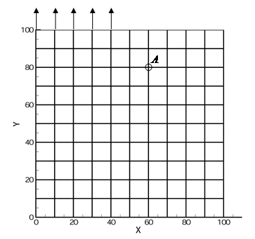
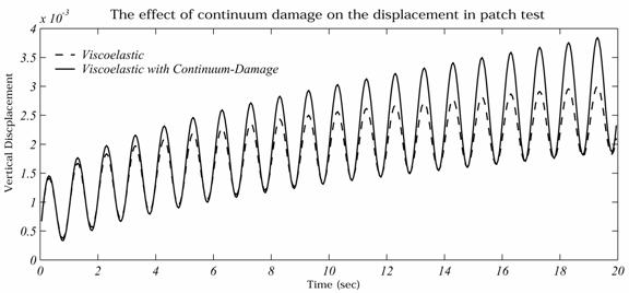
A plot of the above function, assuming a = ^―0.001334 and b = 0.5725, is shown in figure 173. The formulation presented here is not limited to the form of the damage function shown in equation 183. To show the effect of continuum damage, a 10 by 10 patch of 2D plane stress elements has been modeled and is shown in figure 174. The specimen is fixed at the bottom and loaded (in tension) on five nodes at the top. The loading history is sinusoidal as shown in equation 184.

      (184)

Where:

γ = The loading amplitude.

The time history of the vertical displacement for point A () is shown in figure 175. The evolution of damage in the specimen and, consequently, a gradual increment in the displacement amplitude can be seen from the time history. This figure shows that damage has an effect on the response of the material. More quantitative tests on the effect of damage will be performed in the future.

Figure 173. Graph. Damage characteristic relationship used in the finite element implementation of one-dimensional VECD model.

Figure 174. Graph. Layout of the numerical experiment specimen.

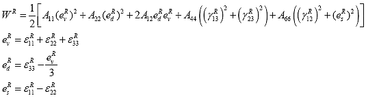
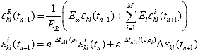
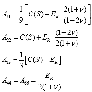
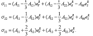
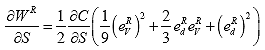
Figure 175. Graph. Effect of continuum damage evolution on the vertical displacement of the test specimen at point A in the test simulation.

6.1.2. Upgraded Constitutive Model

The continuum damage formulation was upgraded to a more rigorous model based on the work of others.⁽⁵⁷⁾ However, a one-parameter damage model was chosen instead of the two-parameter model used in the work because the experimental data needed to characterize a two-parameter damage model are not yet available.

The model assumes that a material is isotropic when undamaged and that the growth of damage under loading leads to local transverse isotropy (i.e., the material has a local axis of symmetry oriented along the maximum principal stress direction). The current framework is formulated for the axisymmetric case but can easily be extended to 3D.

Starting with the work potential theory for an elastic material and making use of viscoelastic fracture mechanics and the correspondence principle for viscoelastic materials, a pseudo strain energy density function, W^R, can be written in terms of the pseudo strains in the local axis as follows: ^(8,9)

      (185)

Where:

_ε11^R, _ε22^R, _ε33^R, _γ12^R, _γ13^R, _γ23^R are the pseudo strains along the local axis.

When the local axis is also a principal axis, the shear strains are zero, and equation 185 becomes the following:

      (186)

In this case,_ε11^R, _ε22^R, and _ε33^R are the principal pseudo strains (which lie in the local axis) with the axis of isotropy oriented along direction 3. These principal pseudo strains are obtained from the pseudo strains along the global axis using standard tensor transformation and knowing the angle between the local axis and the global axis. (For the axisymmetric analysis, the hoop direction is already a principal axis because there are no shear strains along the - plane.) The LVE pseudo strains along the global axis,_εkl^R(t), are calculated from strains along the global axis, _εkl, using the convolution integral.

      (187)

Where:

E_R = Reference modulus that has the same dimensions as the modulus and is usually taken as 1 E(t).

1 E(t) = Relaxation modulus for uniaxial loading.

The calculation of the convolution integral can be very expensive in terms of computation time. In practice, therefore, the pseudo strains are calculated using a state variable approach to reduce the computational expense. When the relaxation modulus of the material E(t) is represented using the Prony series of the form, shown in equation 188, an approximation can be obtained to the convolution integral in equation 187.

      (188)

Where:

E_∞ = The relaxation modulus at t = ∞.

E_i = The Prony coefficients corresponding to the relaxation times, Ρ subscript i.

The pseudo strains along the global axis can be calculated from the following:

     (189)

Where:

ε_klⁱ(t_n+1) (i = 1..M) are the internal state variables that record the history of the material up to time t_n+1, _Δεkl(t_n+1) = ε_kl(t_n+1) - ε_kl(t_n), and Δt=t_n+1-t_n. The pseudo strains at time t_n+1 are calculated based on the strain at times t_n and t_n+1 which are available at the end of the finite element solution step at time t_n+1.

The factors A₁₁, A₂₂, A-₁₂, and A₆₆ are stiffness terms that can be related to a damage function, C(S) as follows: ⁽⁴⁸⁾

      (190)

Where:

ν = Poisson's ratio of the material.

C(S) = A stiffness function that depends on damage in the material.

S = A damage parameter used to track the growth of damage in the specimen.

The principal stresses along the local axis can be found from equation 186 using the following:

     (191)

which gives the following:

      (192)

The stresses along the global axis are then obtained by standard stress transformation and the orientation of the local axis with respect to the global axis.

6.1.3. Damage Model

The growth of the damage parameter S is modeled by extending the concepts of viscoelastic fracture to microcracking.⁽⁸⁾

      (193)

Where:

W^R = Pseudo strain energy density function shown in equation 185.

α = Material-dependent parameter.

From equation 186, the quantity _∂W^R/_∂S can be calculated as a function of pseudo strains in the local axis as follows:

      (194)

Where:

C(S) = Damage function that is assumed to be of the form shown in equation 195, based on experimental data.

      (195)

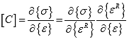
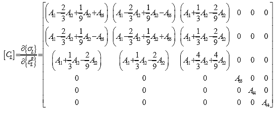
6.1.4. Finite Element Implementation

The finite element solution of the problem requires the material tangent stiffness matrix that is used to assemble the global tangent stiffness matrix used for the solution of the nonlinear system of equations by the Newton-Raphson method. Not to be confused with the damage function, C(S), the material tangent stiffness matrix, [C], is given by the following:

      (196)

Where:

{σ} = {σ_rr, σ θθ, σ_zz, σ_rz} and {ε}={ε_rr, ε θθ, ε_zz, ε_rz}are the stresses and strains for the axisymmetric problem.

[C] = Material tangent stiffness matrix oriented along the global axis. Because the stresses along the global axis are obtained by transforming the stresses in the local axis, it is easier to construct the material tangent stiffness matrix along the local axis and then transform it to the tangent stiffness along the global axis.

The tangent stiffness matrix in the local axis, [C_L], is given as follows:

      (197)

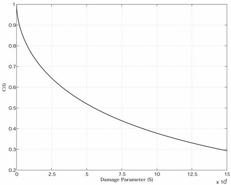
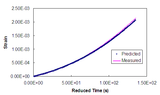
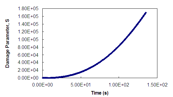
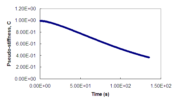
Where:

{σ_L} = {σ₁₁, σ₂₂, σ₃₃, σ₁₂, σ₁₃, σ₂₃} is the stress vector along the local axis.

{ε_L^R} = {ε₁₁^R, ε₂₂^R, ε₃₃^R, γ₁₂^R, γ₁₃^R, γ₂₃^R} is the pseudo strain vector along the local axis.

The pseudo shear strains are zero along the local axis, but the stiffnesses corresponding to them are non-zero. The matrix, [C], can be obtained by transforming [C_L], as shown in the following:

      (198)

Where:

[T_R] = The rotation and permutation matrix that changes the order of the vector components (the axis 3 along the local axis is always oriented along the maximum principal pseudo strain direction) and transforms a vector from the local axis to the global axis.

As seen in equation 193 and 194, the damage growth involves a nonlinear differential equation that can be expensive to solve in a large finite element method (FEM) problem. Hence, a semi-implicit method is used to predict the damage parameter in the next time-step, Sⁿ⁺¹, using the damage parameter in the current time-step, Sⁿ, and the pseudo strain vector in the local axis, {ε_L^R}ⁿ⁺¹, for the next time-step, as follows:

      (199)

This method should provide results similar to those of an exact nonlinear analysis when the time-steps are made small enough.

6.1.5. Verification

The continuum damage material model is verified for a monotonic uniaxial test. The test is part of the uniaxial testing on cylindrical specimens that is conducted for the damage characterization of FHWA mixtures. Verification uses the 5 °C test because there is little or no viscoplastic deformation at this temperature. For the FEM simulation, the cylindrical specimen is modeled as a single quadrilateral (Q4) element that is 150 mm in height and 75 mm in width and is subjected to a uniform axisymmetric loading in the vertical direction. The stress history measured from the test is used as an input for the problem, with the strains calculated by analysis. Horizontal displacements are constrained along the axisymmetric axis of the element, and vertical displacements are constrained along the bottom edge of the element, which results in a uniform state of stress and strain in the element. Predicted strains are then compared against measured strains to verify the FEM implementation of the material model. The damage function is taken as C(S) = exp(-0.001S^0.5737), based on the monotonic test results from several different specimens. The Prony series for the material is obtained from test data for the asphalt concrete mixture used in the testing.

The results of the verification are shown in figure 176 through figure 178. As seen from these figures, the prediction of strain is very good, the damage parameter consistently increases with time and the pseudo stiffness consistently decreases with time. These combined findings verify that the model has been implemented correctly.

Figure 176. Graph. Verification of strain prediction for monotonic uniaxial test using the new continuum damage material model.

Figure 177. Graph. Evolution of damage parameter, S, for the monotonic test.

Figure 178. Graph. Plot of function C(S) with time.

6.1.6. Implementation of Temperature Dependency

The variation of temperature in a pavement has two effects: (1) a change in stiffness of the asphalt concrete and (2) a change of the thermal stresses due to thermal expansion of the material. The thermal stresses are generated in the pavement depending on boundary conditions. These two effects of temperature have been implemented in FEP++.

The change in stiffness in the asphalt concrete due to temperature is taken into account using the concept of reduced time. The reduced time is calculated as follows:

      (200)

Where:

a(T) = Time-temperature shift factor of the material. The time-temperature shift factor is obtained from the characterization of the relaxation modulus of the material using dynamic modulus tests at different frequencies and temperatures. The reduced time is calculated with respect to a reference time and captures the history of temperature variation on the material. The thermal stresses on the material are incorporated by defining mechanical strains, _εm(t), as follows:

      (201)

Where:

{_ε (t)} = Strain in the material.

{α} = Coefficient of isotropic thermal expansion in the material (which is assumed constant for asphalt concrete) and is given by [α,α,α,0,0,0] in three dimensions.

T = Current temperature.

T₀ = Reference temperature at which there are no initial stresses.

The constitutive law for a viscoelastic material undergoing damage is given as follows:

      (202)

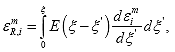
Where:

{_σ} = Stress vector.

[D] = Stiffness matrix that is a function of damage.

{ _m^R} = Vector of mechanical pseudo strain.

The i^th component of the pseudo strain vector is given by the following:

      (203)

Where:

ε_i^m = i^th component of the mechanical strain vector.

E(ζ) = Relaxation modulus of the material characterized at reduced temperature. ζ is computed in accordance with equation 200 and is a function of the temperature history of the material.

6.2. Redesign of FEP++

The older code base of FEP++ was redesigned during the course of the project, leading to a robust, modular, and standards-compliant version. These enhancements greatly improve the maintainability of the code base and significantly reduce the training necessary for a new user.

The FEP++ code base is divided into two major modules, domain and analysis. The following sections discuss the features and functionalities of these modules.

6.2.1. Domain Module

The domain module represents the core finite element component of FEP++. It encompasses the finite element classes that are involved in the modeling of the computational domain. Figure 179 presents a block diagram and the key components of the module. The following sections briefly discuss the main features of the domain module.

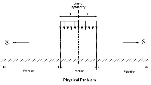
Figure 179. Diagram. Domain module.

6.2.1.1. Material Model

FEP++ provides 2D and 3D models of elastic, viscoelastic, and VECD materials for modeling a pavement layer. Detailed discussion of these models and their implementation is provided in section 6.1.

6.2.1.2. Elements

FEP++ provides two main types of elements, the quadrilateral elements for 2D analysis and the brick elements for 3D analysis of pavements. Also, special elements developed for modeling infinite domains in pavement analysis have been incorporated into FEP++. The following subsection describes the special elements and their efficiency in pavement analysis.

6.2.1.2.1.    Incorporation of special elements for pavement modeling:

A finite element mesh generation methodology for incorporating special elements that reduce the computational costs of pavement analysis has been developed. An accurate mesh of special elements can be difficult to generate because it depends on the characteristics of the load applied. Development of such a methodology may also turn out to be somewhat computationally expensive if it tries to provide greater accuracy than is necessary for the problem at hand. Hence, there is a need to develop a mesh generation methodology that allows the user to easily generate a finite element mesh that models the problem at hand with specified accuracy.

To this end, work is being carried out to generate the best mesh for a specified accuracy through optimization techniques. Generating the best mesh is an involved process that could render it unfeasible for everyday analysis. Therefore, simplified rules will be developed that allow the user to easily generate a mesh that is as close as possible to the best mesh.

A simple example is given below to demonstrate the computational efficiency achieved. Figure 180 shows a layer of elastic material loaded on a rigid base. This layer is infinite in the two horizontal directions. For a strip load of width "2B," the 3D problem can be reduced to a 2D-plane strain problem. Also, symmetry allows that only one half of the problem needs to be modeled. Only the deflection and stresses under the load (the interior region) are of interest here.

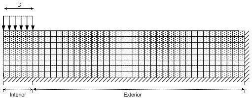
Figure 180. Illustration. Infinite elastic layer on a rigid base.

However, despite the emphasis on the interior region, the exterior region also must be modeled to a sufficient length to simulate the infinite extent of the layer. As the exterior region is extended, the solution in the interior approaches the solution of the physical problem. The objective is to model the physical problem to achieve an accuracy of at least 1 percent. A typical mesh of finite elements used to simulate this physical problem is Mesh-1, shown in figure 181. For Mesh-1, the exterior is four times the extent of the interior and hence needs four times as many finite elements as the interior to achieve an accuracy of 0.86 percent.

If, on the other hand, special elements are used, then Mesh-2 shown in figure 181 is sufficient and provides an accuracy of 0.84 percent. The total number of elements in Mesh-1 is 320, whereas the total number in Mesh-2 is 64. In order to achieve almost the same degree of accuracy as Mesh-1, far fewer special elements are required for Mesh-2. In short, because the computational time is directly proportional to the number of finite elements used to model the problem, Mesh-2 with the special elements is far more computationally efficient when compared to Mesh-1.

The development of a finite element mesh generation methodology that incorporates special elements is now complete. This methodology is being tested on various finite element models to demonstrate its efficacy. Once the results have been verified against theoretical solutions, the mesh generation methodology will be coded into FEP++ to make the discretization both automatic and efficient. (This task will be performed as part of the ongoing cooperative agreement between NCSU and the FHWA.)

Figure 181. Illustration. Finite element mesh required to model the physical problem with 1-percent accuracy without special elements.

Figure 182. Illustration. Finite element mesh required to model the physical problem with 1-percent accuracy with special elements.

6.2.2. Analysis Module

The analysis module handles the generation and solution of the linear/nonlinear system of equations using the domain module. A block diagram of the classes and relationships is shown in figure 183. The following sections discuss the key components of this module.

6.2.2.1. Solution Algorithm

The solution algorithm is the component that acts as a liaison between the domain and analysis modules. This component uses the information in the domain to generate a set of equations that provides the solutions to the problem. Currently, the following static and dynamic analyses of linear, quasilinear, and nonlinear problems are available.

One significant enhancement over the earlier capabilities of FEP++ is the ability to perform quasilinear analysis. This improvement is particularly beneficial in the context of pavement analysis because the VECD material model is quasilinear. By using a quasilinear solver instead of a nonlinear solver, the analysis time is reduced by almost half.

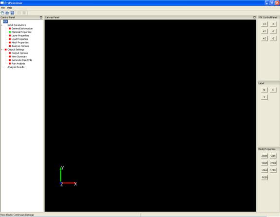
Figure 183. Diagram. Analysis module.

6.2.2.2. Solver

The solver is the workhorse of the module. It is responsible for solving the set of equations generated by the solution algorithm. The solver is also an important component in terms of the capabilities of FEP++ in solving large computational problems because the solver determines the memory requirements and performance output. Any improvements to this module would significantly improve the overall capabilities of FEP++.

Currently, a class of direct methods called Gaussian elimination is used to solve the equations. The objective here is to enhance the component by providing an option to interface with external linear algebra packages to solve the system of equations. The benefit of such a feature would be the ability to use mature, well tested, and highly efficient libraries available in the public domain for performing the analysis. This capability would also reduce further interdependence between the domain and the analysis modules, thereby enhancing the flexibility and elegance of the code.

6.3. PreProcessor

The preprocessor is a graphic user interface (GUI) front end developed for the efficient analysis of pavements using FEP++. The motivation behind the tool is to provide the user with a simplified and intuitive interface to FEP++ for pavement analysis. The tool can be used either to run an analysis directly or to generate the input files for FEP++. It also has visualization capabilities to view the mesh discretization, which makes it easy for the user to verify the input data for the analysis. Figure 184 shows a screenshot of the main window in the preprocessor.

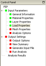
Figure 184. Screen capture. Main window of the preprocessor.

As labeled in figure 184, the main window is divided into three functional units, the control panel, the canvas panel, and the popular open-source library called Visualization Toolkit (VTK) control panel, described below.

The left-hand unit is called the Control Panel. This panel contains the controls to invoke the data-entry windows and other operations related to the analysis. Each control is either red or green, indicating the current state of the analysis. For controls corresponding to data entry operations, green indicates that no user action is required. Green, therefore, could either signal that the data entry has already been completed or that it is preset with a default set of parameters. Red indicates that some action is required from the user. The data input is considered complete only when all the controls in the input parameters block (figure 185) are green.

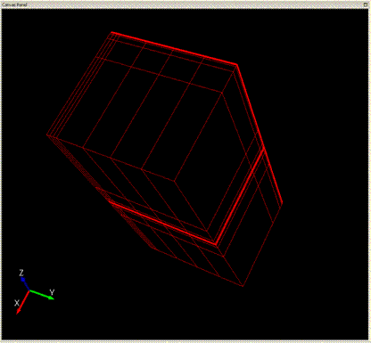
Figure 185. Screen capture. Control panel.

The middle unit is called the Canvas Panel. This panel is used for the visualization of the mesh discretization and the solid model of the pavement. The underlying graphical engine used to render the graphics is VTK. This toolkit was chosen for its stable and mature set of high-level graphical libraries. Also, it is popular and widely used in the open-source and scientific community. Figure 186 shows a sample mesh discretization in the canvas panel.

The rightmost unit provides the controls for the visualization operations supported in the preprocessor, e.g., zoom, pan, etc., and is called the VTK control panel. The following operations are currently supported:

• Projections along a plane, e.g., along the x-y plane.
• Image operations, such as zoom, pan, and rotate.
• Display nodes and cell numbers on the mesh.

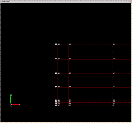
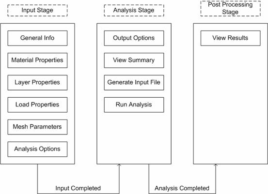
The results of these operations are displayed in the view window. Figure 187 shows the zoomed version of a 2D mesh with node numbers displayed. The visual feedback from these windows is useful to verify the data inputs to the analysis. The different stages involved in performing a pavement analysis and the ways that the various analytical pieces fit together are outlined in figure 188.

The input stage corresponds to the data-entry windows that receive the input data from a user (i.e., it shows the list of data that needs to be entered by the user). The analysis stage shows the list of options available to the user once the input stage is complete. The postprocessing stage again shows the options after the analysis is completed successfully. The above mentioned stages are discussed in detail in the following sections.

Figure 186. Screen capture. Mesh discretization.

Figure 187. Screen capture. Zoom operation on a mesh.

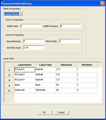
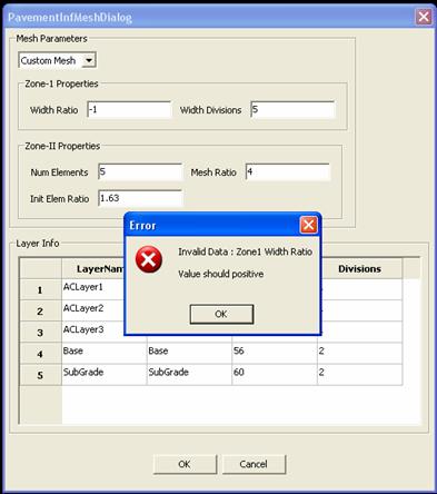
Figure 188. Diagram. Stages involved in an FEP++ analysis.

6.3.1. Input Stage

As discussed in the previous section, this stage corresponds to the data entry by the user. Each main input data entry for FEP++ corresponds to a data entry window. The user manual, with a detailed explanation of each of the data entry windows, is provided in the appendix of this report. Figure 189 shows a data entry window for entering the mesh discretization parameters for a pavement.

The data entry windows have been designed in a modular way, and effective error validation schemes have been incorporated to ensure consistent input data. Each data entry window has a data class associated with it that enforces the validation and consistency checks. There are two levels of error validations that are carried out at each data entry window, namely syntactic and semantic errors. The syntactic errors refer to invalid data entries, and they are checked by the data entry windows themselves, whereas the semantic errors refer to consistency check failures imposed by the data classes.

Once the data entry is complete for a particular block, it is validated against the checks provided in the data classes. If the validation is successful, the next data entry window can be accessed. If it fails, appropriate error messages are shown, and the user is asked to modify the incorrect data. Figure 190 shows a typical error dialog that is displayed when a consistency check fails.

Figure 189. Screen capture. Sample data entry window.

This sequential data entry process may seem to be somewhat limiting, but it greatly simplifies the maintenance of consistency in the input data. Also, by strictly enforcing these checks in the software, there is less scope for input data corruption.

6.3.2. Analysis Stage

Once the data entry has been completed, the analysis section in the control panel turns green, signaling that the actions in the analysis stage can now be performed. The following sections discuss the actions that can be performed at this stage.

6.3.2.1. Setting the Output Options

Output options can be used to control the results that are generated by FEP++. For example, FEP++ can be configured to output data that correspond to a particular region in the domain. These options are essentially used to control the amount of data output by FEP++.

6.3.2.2. Viewing a Summary of the Input Data

The preprocessor can be used to create a user-readable report of the input data entered for an analysis. This report can be used to verify the final state of all the input data before beginning a simulation.

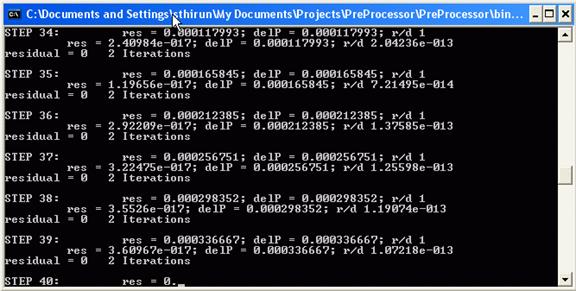
Figure 190. Screen capture. Error dialog for a semantic error.

6.3.2.3. Generating an FEP++ Input File

The preprocessor can be used to generate input files for FEP++ for different configurations that can then be saved to a remote location. This feature is helpful if the user wishes to perform multiple analyses in a script without any user intervention.

6.3.2.4. Running an Analysis

Running an analysis is the final step in pavement analysis. The analysis can be started only after the run analysis option in the control panel turns green. The preprocessor uses the user input to create an input file to FEP++ and invokes it with the generated input file. The preprocessor creates a separate instance and displays the progress of the analysis in a window, as shown in figure 191 .

Figure 191. Screen capture. Analysis run-time window.

6.3.3. Postprocessing Stage

After an analysis is completed, the run-time window shown in figure 191 exits, and the results option on the control panel turns green, indicating that result files have been generated that can be viewed with a postprocessor. On choosing view results, the default postprocessor is invoked to view the results.

6.4. PostProcessor

The postprocessor is an external tool for visualizing the results of the pavement analysis. Currently, Tecplot^® serves as the default postprocessor, but efforts to provide support for other open-source data visualization tools are underway. It has been decided that the VTK format will be used for the output file format and that MayaVi, a stable open-source python-based viewer that is popular in the finite element community, will be used as a suitable viewer. The support for external tools will be completed in the next project.

Previous | Table of Contents | Next