Chapter 7. A Sample 3D Pavement Simulation Using FEP++
As mentioned in the previous chapter, FEP++ has full support for 3D finite element analysis of elastic and viscoelastic materials. This chapter discusses the details of a 3D analysis performed using FEP++ to study the effects of temperature, material, and wheel speed on ALF pavements. The following sections discuss the analysis details and the results.
7.1. The Input Data
The pavement was modeled as a 3D cuboid, and the details are shown in table 23. A single moving wheel load with the parameters shown in table 24 is used in the analysis. The behavior of the pavement was studied for the effects of temperature, material, and wheel speed. The following subsections discuss the simulations and the results in detail.
Table 23. Properties of pavement.
| Depth of AC Layer |
46 cm |
| Pavement Length |
296.5 cm |
| AC Material |
ALF Control/
ALF SBS |
| Subgrade Type and Stiffness |
Infinite Subgrade, 86 MPa |
| Ambient Surface Temperature |
Winter (-5 °C)/
Summer (38 °C) |
Table 24. Properties of moving wheel load.
Contact Pressure |
758 kPa |
Load Area |
19.65 cm by 17.79 cm |
Wheel Velocity |
13.41 m/s/26.82 m/s |
7.2. Effect of Temperature
To simulate the effect of temperature, the analysis was performed at representative temperatures for winter and summer. The temperature distribution across the depth was found from simulations with the Enhanced Integrated Climatic Model (EICM). For these simulations, a typical pavement cross section was used with the Raleigh, NC, climatological database. The exact temperature variation is shown in figure 192.
The strains were expected to be larger during the summer as compared to the winter because the material stiffness was smaller at higher temperatures leading to larger deformations. Also, the material was expected to display a higher degree of viscoelasticity at higher temperatures while displaying higher elasticity at lower temperatures.
Figure 193 through figure 198 show the strain distributions for the above analysis when the wheel load reached the center of the pavement. The temperature distribution across the depth is also shown in each of the figures. Figure 193 and figure 194 show the vertical strain distribution, and, as expected, the strains were smaller for the winter loading than for the summer loading. Also, the strain distribution was more or less symmetrical around the wheel location for winter loading as compared to the summer loading which showed some residual strain from the passing of the wheel. Thus, the viscoelastic behavior was more prominent at higher temperatures.
Figure 195 and figure 197 show the strain distributions for longitudinal and transverse strains. The strains were consistently higher in the case of summer loading than in winter loading, and the elastic nature of the material (symmetry about the wheel) was more prominent during the winter loading. Thus, the results of the FEM analysis of the effects of temperature on the material properties agreed well with the expected outcome.
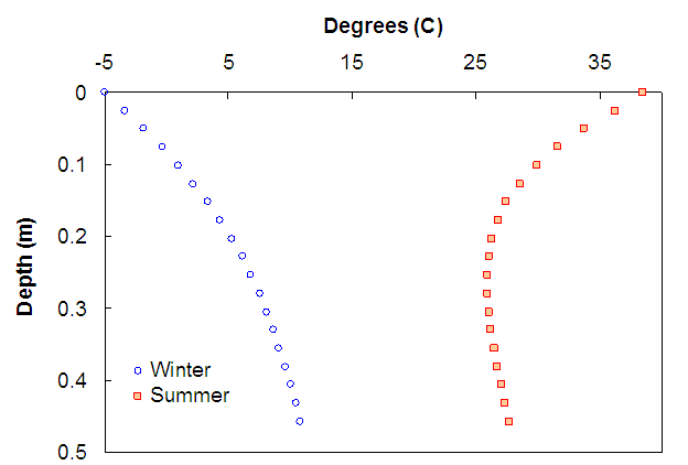
Figure 192. Graph. Temperature variations used for simulations.
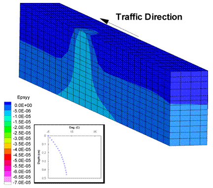
Figure 193. Illustration. Vertical strains in winter.
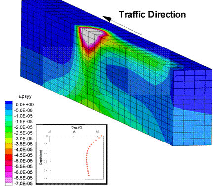
Figure 194. Illustration. Vertical strains in summer.
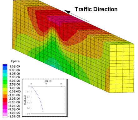
Figure 195. Illustration. Longitudinal strains in winter.
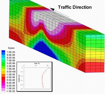
Figure 196. Illustration. Longitudinal strains in summer.
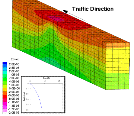
Figure 197. Illustration. Transverse strains in winter.
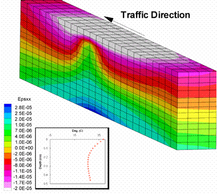
Figure 198. Illustration. Transverse strains in summer.
7.3. Effect of Material
The effect of material properties on pavement behavior was analyzed next. Pavements under summer conditions, with the ALF Control mixture and the ALF SBS mixture for the asphalt concrete layer, were used for the simulations, and a wheel speed of 26.82 m/s was applied. Because the SBS pavement was less stiff compared to the ALF Control pavement, the strains were expected to be higher for the SBS pavement.
Figure 199 through figure 204 show the strain distributions for the above analysis when the wheel load reached the center of the pavement. Figure 199 and figure 200 show the vertical strain distribution; the SBS pavement had higher strains compared to the Control pavement. Also, the strains in the SBS pavement located away from the wheel location were higher, indicating that the strains in the SBS pavement took longer to recover from the passing of a wheel than those of the Control pavement.
Figure 201 and figure 202 show the longitudinal strains for the two mixtures. Again, the strains were larger for the SBS mixture than for the Control mixture, leading to larger regions of tension and compression.
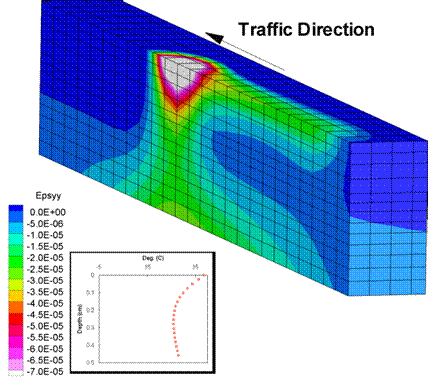
Figure 199. Illustration. Vertical strains for Control mixture.
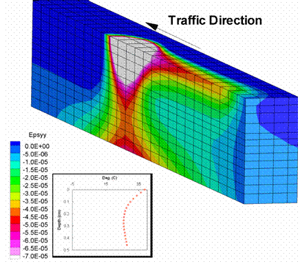
Figure 200. Illustration. Vertical strains for SBS mixture.
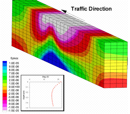
Figure 201. Illustration. Longitudinal strains for Control mixture.
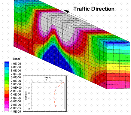
Figure 202. Illustration. Longitudinal strains for SBS mixture.
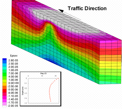
Figure 203. Illustration. Transverse strains for Control mixture.
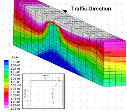
Figure 204. Illustration. Transverse strains for SBS mixture.
Figure 203 and figure 204 show the transverse strains. Again, the strains were larger for the SBS mixture than for the Control mixture. Also, the region of maximum tension at the bottom of the pavement was much larger for the SBS pavement than for the Control pavement. The area of influence on the surface of the pavement was higher for the SBS mixture than the Control mixture.
Again, the results were as expected. The SBS pavement deformed more than the Control pavement, and the area of influence was larger due to its lower stiffness.
7.4. Effect of Wheel Speed
Finally, the effect of the wheel speed on pavement behavior was analyzed. The analysis was performed on a pavement using the ALF Control mixture for the asphalt concrete layer under summer conditions for two cases with wheel speeds of 13.41 and 26.82 m/s, respectively. Because the viscoelastic model was quasistatic, dynamic effects (acceleration/velocity) were not considered, and the effect of the wheel speed essentially affected only the load duration at each point on the pavement. Thus, the effect of a slower wheel speed could be a longer duration of the load pulse and, consequently, larger vertical strains compared to a faster wheel speed. Also, the slower wheel load could create a larger area of influence because the material recovery time may be comparable to the wheel passing time.
Figure 205 through figure 210 show the strain distribution for the analysis when the wheel load reached the center of the pavement. Figure 205 and figure 206 show the vertical strains, which were slightly larger for the slower wheel speed. The memory effect was slightly more pronounced for the slower wheel speed, as shown by the larger strains in the pavement region passed by the wheel.
Figure 207 through figure 210 show the longitudinal and transverse strains; these strains displayed similar characteristics to the vertical strains, although the effects were much less pronounced. The vertical strains seemed to be most sensitive to the wheel speed.
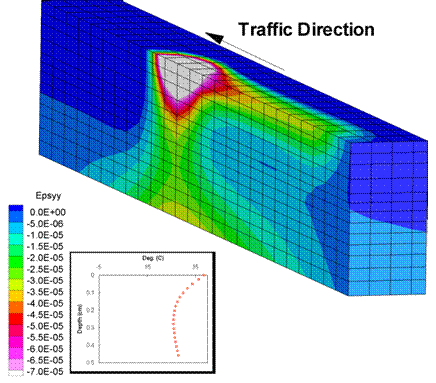
Figure 205. Illustration. Vertical strains for a wheel speed of 13.41 m/s.
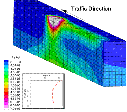
Figure 206. Illustration. Vertical strains for a wheel speed of 26.82 m/s.
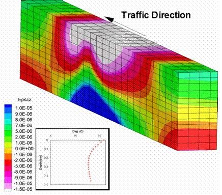
Figure 207. Illustration. Longitudinal strains for a wheel speed of 13.41 m/s.
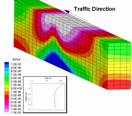
Figure 208. Illustration. Longitudinal strains for a wheel speed of 26.82 m/s.
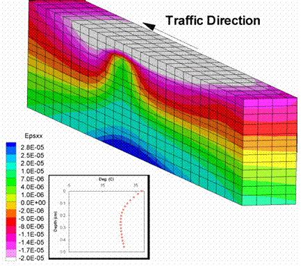
Figure 209. Illustration. Transverse strains for a wheel speed of 13.41 m/s.
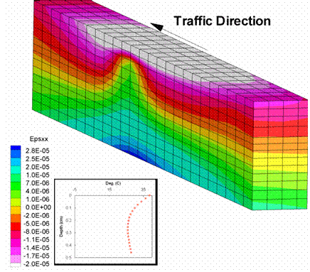
Figure 210. Illustration. Transverse strains for a wheel speed of 26.82 m/s.
|


