Estimating Cumulative Traffic Loads, Volume II:
Traffic Data Assessment and Axle Load Projection for The Sites With Acceptable Axle Weight Data, Final Report for Phase 2

CHAPTER 2. PROCEDURES FOR TRAFFIC DATA ASSESSMENT AND PROJECTION (cont'd)

Step 5–Preparation of LTPP Traffic Feedback and Resolution Packages for All Participating Agencies

Once the package was developed through the review and consultative process outlined previously, a procedure was established to produce a package for each participating agency and to send it to RCOs for review. A substantial part of the package was produced as a customized printout of data stored in the IMS database. The assessment of data quality, the selection of data for projection, and the development of the projection models were done on a section–by–section basis using engineering and analytical judgment. The following activities were carried out to develop traffic projections:

• Assessment of traffic data.
• Projection of truck volumes.
• Development of base annual spectra.
• Assignment of initialprojection confidence codes.
• Computation of annual axle load spectra.

These activities are described in the following sections under separate headings; however, the first four activities were intertwined.

The following principles applied to all traffic data assessment and projection work.

• Close attention was paid to whether the data and traffic projections encountered in the course of the work were reasonable. For example, when working with truck volumes, the corresponding highway classification, number of lanes, and AADT volumes reported for different years on the same site or on similar sites were noted to identify potential idiosyncrasies.
• All activities requiring engineering and analytical judgment were carried out by at least two members of the project team. Typically, one project team member carried out the task and the second member independently reviewed the outcome of the task. Any differences were discussed to reach a consensus.
• The initial projections were done with the understanding that they will be reviewed by the participating agencies. It was considered more constructive and beneficial for the projection if the project team were proactive and developed the initial traffic projection whenever possible, rather then to ask agencies first for more data or for directions. Consequently, for example, only meager data and engineering judgment were sometimes used to propose the truck volume projection model.
• The traffic data assessment and projection work was done for all sites belonging to an agency at the same time. This approach enabled the project team to cross–compare trends in data to identify data discrepancies and to develop solutions and for their resolution.

Assessment of Traffic Data

A general assessment of data quantity and quality for all LTPP sites within the agency was carried out as part of the preparation of the initial overall feedback and resolution report. Because traffic data for all LTPP sites within an agency were assessed at the same time, the process benefited from cross–comparison of trends observed on all sites. The site–specific assessment of data quantity and quality followed similar themes as those used to develop the initial overall feedback and resolution report: evaluation of missing data, location of sections, traffic volumes, vehicle classification (operation of AVC equipment), and axle weights (operation of WIM scales), and was based on the site–specific reports.

Observations regarding traffic data that were considered to be of interest to the participating agencies, or questions that the project team members had for the representatives of the participating agencies, were included in part 6 of the Blue Sheets (figure 3).

In some respects, the assessment of traffic data carried out as part of this study resembled the traffic data QA process recommended in the LTPP Traffic QC User's Guide.^[12] However, there were fundamental differences between the quality control (QC) recommended by the guide and the traffic data assessment process carried out as part of the traffic projection process. The fundamental differences were in the timing and the outcome of the two activities, and in the length of the time period for which the traffic data were assessed.

The QC should be carried out a few days or weeks after traffic data are collected so that an appropriate corrective action (such as equipment calibration) can take place in a timely manner. Traffic data assessment carried out in this study took place many years after the data were collected. The QC process may result in the removal of nonsensical data, but no data were removed from the database as part of this study. However, nonsensical data were identified and were not used for traffic projections. Finally, the previous QC process evaluated traffic data for only relatively short time periods, such as day, week, month, or quarter, without examining long–term trends. Traffic data assessment done in this study evaluated only annual data, but evaluated trends in annual data for all in–service years.

The type of traffic data assessment done in this study is not a replacement for the appropriate QC process. The assessment process used was necessitated by the quality of available traffic data and the need to provide the initial traffic projection for the development and calibration of the 2002 Pavement Design Guide.^[7] Traffic data used in this study still need to be evaluated using a basic QA process.

Projection of Truck Volumes

To estimate traffic loads for all in–service years, it was necessary to estimate the AADT volumes for all years the pavement was in service. The available historical and monitoring truck volume data had to be "backcasted" (to years before the sites became part of the LTPP program), interpolated (for the interim monitoring years without monitoring data), and forecasted (for years after the data are no longer collected), as shown schematically in figure 11.

The AADT volumes for all in–service years were estimated using a projection model. The AADT projection model was also used to obtain annual projection factors required for the calculation of the annual axle load spectrum (see equation 1).

Figure 11. Projection of truck volumes using historical and monitoring data.

Figure 6 provides an example of the AADT truck projection model for site 285805. Twelve other examples of the projection model were provided in the Phase 1 report.^[1] The table in figure 6 lists historical, monitoring, and projected AADT volumes from 1975 when the pavement was open to traffic to 1998. Also listed are the projected growth percentage and the projected growth factor. The projected growth percentage, indicating the historical rate of growth in truck volumes, was provided to facilitate the review of the projection models by the participating agencies. The projected growth factor, also referred to as "Annual Projection Factor" in equation 1, is a multiplier that was applied to the base annual spectrum to obtain projected annual axle load spectra for each year the section was in service. Projected growth factors were used to scale overall truck volumes up or down compared to base conditions and to account for traffic growth for different years.

The development of the AADT truck projection model followed the procedures developed in Phase 1 and documented in reference 1. Briefly, the available historical and monitoring annual truck volumes were plotted separately for each site and analyzed to determine their statistical characteristics. Plots of annual volumes often revealed considerable variation. Typically, simple regression models would fit the data best. However, least square regressions were not carried out because the technique cannot accommodate many considerations that were used to develop the projection model, and would not provide more meaningful results.

Some considerations used to develop the AADT truck projection models are summarized here.

• The monitoring AADT truck volumes, based on measured data, should be more reliable than historical volumes based on estimated data. In situations where historical and monitoring truck volumes did not match, the projection model placed more emphasis on the monitoring data and followed the monitoring data more closely than the historical data. The emphasis on the measured truck volumes is shown in the projection model in figure 6.
• Monitoring annual truck volumes based on measurements carried out during a substantial portion of the year should be more reliable than monitoring annual volumes based on short–duration measurements. The number of days and months during which AVC and WIM data were collected was known for all monitoring years up to 1998 and was listed on the bottom of Annual Traffic Projection Sheet (figure 5).
• The development of the projection model considered not only the trends in AADT truck volumes, but also the trends in AADT vehicle volumes, truck factors (TFs), and ESALs summarized in the Annual Traffic Projection Sheet (figure 5).
• Consistency of the historical estimates and the relationship between the historical and monitoring volumes for all sites within the agency. For example, if the historical truck volume estimates matched the subsequent monitoring volumes well for the majority of the sites within the agency, the historical volumes would be given greater weight for the sites where the match between the historical and monitoring volumes was poor.
• To initiate the traffic projection process and to provide a concrete example of the initial model for consideration and comments by the participating agencies, the AADT truck projection models were developed for all LTPP sites with at least some truck volume information. For example, if the AADT truck volume was available for only one monitoring year in 1998 and the section was opened to traffic in 1991, we would still provide truck volume estimates for all years between 1991 and 1998. The volume reported for 1998 would be assessed for reasonableness by considering other available data, such as AADT volumes, traffic volumes on similar sites in the same agency, the number of lanes, and highway classification. The projected growth in truck volumes between 1991 and 1998 would be based on the growth rate at similar sites in the same jurisdiction. Because this information was unavailable for a few sites, we used a 5 percent historical growth rate in truck traffic for interstates and major highways and a 2 percent rate for other highways. These rates were established by examining vehicle travel statistics available at FHWA's Web site, www.fhwa.dot.gov/ohinstat.htm. Subsequent analysis of LTPP data (presented in table 13, later in this report) confirmed that the selected growth rates are reasonable. It needs to be emphasized that the growth rate estimates were made to initiate the projection process and to submit a concrete projection for the review and comment by the participating agencies. Agencies were asked to verify the proposed growth rates using local information.
• Specific attention was paid to the influence of unclassified vehicles reported as Class 14 vehicles. The number of Class 14 vehicles strongly influenced total truck volumes on many sites in several agencies. After analysis of trends in truck volumes, Class 14 vehicles were usually attributed to passenger cars. Example of such analysis for three Minnesota LTPP sites is shown in figure 12. The treatment of Class 14 vehicles used in this study should be considered to be an interim measure. For some agencies and sites, consideration should be given to re–processing raw traffic data to distribute the Class 14 vehicles among the 13 vehicle classes.

Development of Base Annual Spectra

The objective of the development of base annual spectra was to obtain the annual axle load distribution or distributions that best reflect the axle loads on the site. The development of base annual spectra was the most challenging part of the entire projection process. The shape of the base annual spectrum (i.e., the normalized base annual spectrum) remained the same for all years. To obtain annual axle load spectra for all in–service years, the base annual spectrum was multiplied by a scale factor (annual projection factor) to reflect the historical changes in truck volumes (equation 1).

The annual axle load spectra showed a large variation in the amount and quality of monitoring axle load data. For example, some spectra had unexpected shapes with very few loaded axles, others had a large proportion of apparent axle overloads. Annual spectra also varied considerably from year to year. Reasons for the variation in and unusual shape of the spectra include:

• Length of the sampling period–The number of days per year during which the WIM scales were operating varied from site to site and year to year. The length of the WIM data– collection period for monitoring years up to 1998 was reported on the bottom part of the Annual Traffic Projection Summary Sheet (figure 5). The shortest period necessary for obtaining annual axle loads spectra was 24 consecutive hours. A spectrum based on several months of data may be quite different from one based on only a few days of data.
• Equipment errors–These errors, caused by equipment limitations, can result in bias and cannot be remedied without changes to the equipment. It is possible that some occurrences with the large numbers of Class 14 vehicles were due to equipment errors.
• Calibration errors–These errors are caused by inaccuracies resulting from the way the physical response of the equipment to the passing vehicles is transformed into units of weight. After the initial calibration, the scales may have been allowed to drift. Thus, the axle load spectrum based on the first year of operation may be different from the spectra obtained for the subsequent years. Automatic calibration based on the weight of steering axles of Class 9 vehicles is not always reliable.
• Changes in traffic patterns–Annual axle load spectra for sites with low truck volumes may be significantly influenced by changes in the location and operation of nearby large truck traffic generators (e.g., by the construction of a large subdivision or by opening of new industry).
• Natural variation–Traffic loads naturally vary from year to year due to economic and other factors.

Figure 12. Comparison of AADT volumes for Class 14 vehicles with AADT volumes for all trucks.

Selection of the base annual spectra was carried out by examining all available monitoring data for a given site, including all available truck class and axle load distributions. Graphic displays of traffic data, contained in the site–specific reports, were used for this purpose. The assessment considered the shape of the spectra (e.g., presence and location of peaks in the tandem axle spectra) and the differences and trends among the available spectra.

The main technique used to assess axle load spectra was the expectation that many large trucks operate either fully loaded or empty. The loaded peak is usually below the maximum allowable load because shippers may not know the exact weight of the empty trucks that will transport shipments. Consequently, they prepare or partition shipments with a margin of safety (so that the shipment and the weight of the truck will not exceed the allowable axle weight and gross vehicle weight limits). For example, if the allowable axle load on tandem axles is 15,436 kg (34,000 lb), the majority of fully loaded trucks should have tandem axle loads in the range of 14,074 to 14,982 kg (31,000 to 33,000 lb). Typical values for unloaded and fully loaded axles, together with Federal axle load regulations, are summarized in table 6.^[13]

Table 6. Characteristic values of axle load spectra.

As outlined in the Phase 1 report, there are many exceptions to the Federal vehicle weight regulations on the State and Provincial levels.^[1] The enforcement of vehicle weight regulations also plays an important part. The values provided in table 6, therefore, are only typical guideline values.

The basic procedures used to obtain the base annual spectrum included:

• Computing the mean of all available annual axle load spectra.
• Computing the mean of selected annual axle load spectra.
• Selecting one or two annual axle load spectra.
• Rejecting all available annual axle load spectra.

An additional computational provision was made for sites with many years of reliable annual axle load spectra. It is possible to utilize two base annual spectra for the traffic load projection on one site. The first base spectrum can be used to represent traffic loads during the years before the installation of a WIM scale and during the initial operation of the scale; the second spectrum can be used to represent traffic loads for the most recent years with and without WIM scale data. Both the first and the second base annual spectra can be the averages of several annual spectra. However, this provision was not used for any LTPP site because its use was not warranted by quality of available axle load data.

Mean of all Available Annual Axle Load Spectra

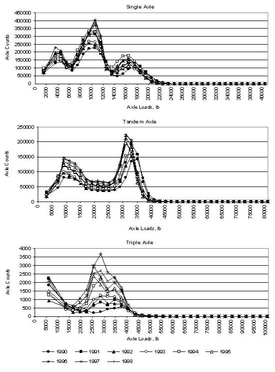
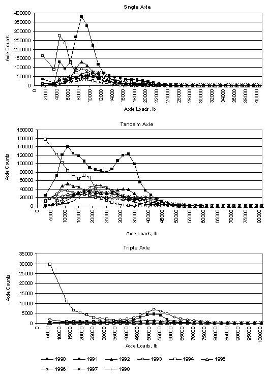
A mean of all available annual axle load spectra was used if the mean spectrum was considered to be the best representation of traffic loads for the given site. An example of annual axle load spectra that were averaged to obtain the base annual spectrum is shown in figure 13 (for California site 063042, located on Interstate 5 south of Sacramento, CA). The base annual spectrum was obtained as a mean value of the annual spectra for 1990 to 1998, inclusively.

Mean of Selected Annual Axle Load Spectra

A mean of selected annual axle load spectra was used if some of the available annual spectra were considered to be outliers (for example, because of the large percentage of very excessive loads, or because the expected loaded and unloaded peaks were not present) and could not be used to determine the base annual spectrum. The base spectrum was calculated as the mean of the remaining spectra. An example of establishing the base annual spectrum as a mean of selected annual spectra is shown in figure 14 (for site 185518 on a rural interstate in Indiana).

The base annual spectrum for the site in figure 14 was calculated as the mean of annual axle load spectra for three years (1991, 1992, and 1995). The truck class distribution for the site was examined and was considered to be stable throughout the monitoring years. Consequently, the annual spectra were expected to be similar for all monitoring years.

Specific reasons that several of the annual axle load spectra shown in figure 14 were not used for calculating the base annual spectrum were:

• 1993 spectrum: The spectrum is flat and contains a relatively large number of overloaded tandem axles; the spectrum for single axle loads has no peak.
• 1994 spectrum: The spectrum is on the margin of being acceptable, and it is possible that other analysts would include this spectrum in the calculation of the base annual spectrum. However, it includes a relatively large number of tandem axle overloads (tandem axle weights exceeding 15,436 kg (34,000 lb)). Adding the 1994 spectra–to the already selected spectra for 1991, 1992, and 1995–would have only a small influence on the resulting base annual spectrum and on the cumulative axle loads.
• 1996, 1997, and 1998 spectra: The peak for single axles is below 4,540 kg (10,000 lb), and there are no peaks for tandem axles corresponding to the loaded and unloaded axles.

Another example of establishing the base annual spectrum as a mean of selected spectra is provided in figure 8, showing five annual axle load spectra for Mississippi site 285805. Initially, the base spectrum was calculated as the mean of 1992, 1993, 1994, and 1995 spectra. The 1996 spectrum was not used for the initial projection because it was considered to be an outlier. Its peak for the loaded tandem axles was about 2,270 kg (5,000 lb) higher than the peaks of the other four annual spectra (14,528 kg (32,000 lb) compared to 12,228 kg (27,000 lb)). However, in response to a subsequent review carried out by a representative of the Mississippi DOT, the 1996 annual spectrum was included in the calculation of the reviewed base annual spectrum. The utilization of review comments received by the participating agencies is discussed in step 8 (" Implementation of Review Comments Received from Participating Agencies").

Selection of One or Two Annual Axle Load Spectra

Many sites had only one or two annual axle load spectra that were considered suitable for the development of base annual spectrum. An example of such a situation is provided in figure 15 for site 124057, located on a rural Interstate 75 east of Tampa, FL. From the eight annual spectra available for this site, only axle load spectra for 1991 and 1992 were used for the projection. The reasons for the rejection of the remaining spectra (for years 1993 through 1998) were similar to those given for the rejection of the spectra in figure 14.

The 1991 and 1992 spectra have similar shapes but have different magnitudes: the 1992 spectrum is based on a much smaller number of trucks than the 1991 spectrum. Because the projection process utilizes the normalized spectra, the difference in magnitude does not influence the calculation of annual base spectra. It should be pointed out that the allowable tandem axle load in Florida is [DH1]  19,976 kg (44,000 lb)even though the maximum allowable gross vehicle weight is still 36,320 kg (80,000 lb). Consequently, the 1991 and 1992 spectra (given in figure 15) used for the development of base annual spectra do not contain many overloads.

Rejection of All Available Annual Axle Load Spectra

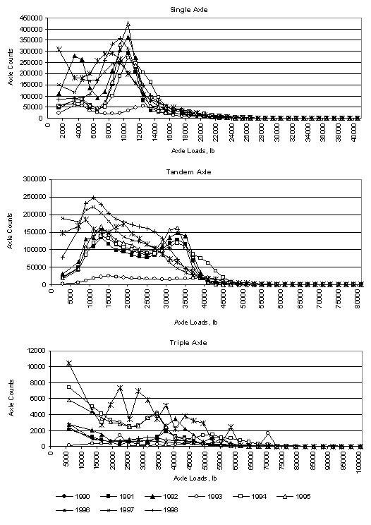
For many sites, all available monitoring annual axle load spectra were judged to be inappropriate for the development of base annual spectra, and thus for the projection of traffic loads. The main consideration in not using the available monitoring data was the possibility that their use would result in a larger error in the projected traffic loads than the use of surrogate data such as site–related, regional, or generic axle load spectra. See figure 16 for an example of a site for which all available spectra were rejected.

063042 Annual Load Spectra

1 lb = 2.202 kg

185518 Annual Load Spectra

1 lb = 2.202 kg

Figure 14. Use of the mean of 1991, 1992, and 1995 annual axle load spectra to obtain base annual spectrum.

124057 Annual Load Spectra

1 lb = 2.202 kg

473104 Annual Load Spectra

1 lb = 2.202 kg

Figure 16. Rejection of all available annual axle load spectra.

Figure 16 shows five annual axle load spectra for site 473104 in Tennessee located on a rural major collector highway. The 1995 and 1996 spectra contain an unreasonable number of overloaded tandem axles. The main problem with the 1992, 1993, 1994, and 1995 spectra is probably the small number of observations (weighted trucks) used to develop the spectra.

Additional information on the indicators used to decide whether individual axle load spectra were suitable for the projection of traffic loads is discussed next.

Assignment of Initial Projection Confidence Codes

The purpose of developing projection confidence codes was to characterize the uncertainty associated with traffic load projections. Such characterization is useful for the development of pavement performance models and for the development of pavement design procedures that incorporate reliability concepts.

The level of confidence in the initial traffic projections has been expressed in the form of initial traffic projection codes that have been assigned to all LTPP sites. The following three codes were used to characterize the level of confidence associated with initial traffic projection results:

• IA–Initial acceptable projection results.
• IQ–Initial questionable projection results.
• IN–Initial not available projection results.

The traffic projections were classified according to the confidence codes to provide guidance to the pavement analyst regarding overall expected accuracy of traffic projections. However, the actual accuracy of traffic projections is unknown because the actual traffic loads that went over the sites during the time the pavement was in service is not known. To provide guidance to the pavement analyst, the following approximate interpretation of the initial projection confidence codes has been provided:

• IA–Cumulative ESAL estimates are probably within ±50 percent of the actual cumulative ESAL values.
• IQ–Cumulative ESAL estimates are probably off by more than ±50 percent from the actual cumulative ESAL values, but are probably better than the estimates based entirely on surrogate (regional or generic) data. Cumulative ESAL estimates are probably within ±100 percent of actual ESAL values.
• IN–Axle load estimates could not be provided at this time.

The initial traffic projection codes were assigned subjectively using engineering judgment and considering:

• Site–specific historical and monitoring traffic data.
• Agencywide historical and monitoring traffic data.
• Other data such as highway location, functional class, and total number of lanes.

Only three traffic projection codes were used because of uncertainties inherent in the traffic projection process caused by the amount and quality of traffic data. Traffic data available for the projection of traffic loads received only a cursory QC and QA review, and include good, marginal, and erroneous data.

The initial projection of traffic loads and the assignment of the projection codes were carried out for all sites within the agency at the same time. The projection process utilized agencywide trends and similarities in historical and monitoring data. This was achieved, for example, by comparing traffic loads reported for nearby sites (as shown in table 3) and similar sites, or by comparing the match between historical and monitoring truck volumes, or between historical and monitoring TFs, for all sites. When weighing the information provided by historical and monitoring data, the extent, consistency, and quality of the agency's historical monitoring data were taken into account.

An agency's consistency and reliability in providing historical traffic load estimates, particularly estimates that were in good agreement with the subsequent monitoring data, imparted additional confidence in the traffic projections. For many sites, the number of historical years exceeded the number of monitoring years, so the reliability of historical traffic estimates played an important role in assigning projection confidence codes. For example, figure 5 shows that for site 285805 there were 17 historical years (1975 to 1991) and 7 monitoring years (1992 to 1998, even though 1997 and 1998 had no monitoring data). The reliability of cumulative traffic load estimates (from 1975 to 1998) at this site depends also on the reliability of historical data.

The level of confidence was linked to the accuracy of traffic projections even though the accuracy of traffic projections cannot be determined and will remain unknown. It is believed that the comparison of the projected traffic loads with the actual expected traffic loads is more meaningful than the comparisons of the projected traffic loads with a relative reference, such as the estimated traffic loads based on monitoring data, because the relative reference also may be subject to error.

The level of confidence was related to the cumulative ESALs. Cumulative rather than annual ESALs were used to avoid the influence of annual variation in traffic loads that can occur by chance alone, or can be caused by other reasons, such as special events.

The assignment of the initial projection codes using judgment was a complex task that used subjective interpretation of all relevant information provided by historical and monitoring data. To minimize the subjectivity involved in assigning the confidence codes for the initial traffic projections, researchers ensured that:

• The assignment of codes was based on guidelines.
• At least two project team members were involved in assigning codes for each section. The experience with pavement condition rating (which is also done subjectively using guidelines) indicates that the use of multiple raters has a positive influence on the variability of pavement condition rating.^[14]

The guidelines for assigning projection confidence codes described in the following section are organized under the main headings of "Guidelines for Assigning IA, IN, and IQ Codes," respectively, and under the subheadings of "Location, Truck Volumes, Truck Classification, and Axle Weights." However, the assignment of the projection confidence codes considered simultaneously all traffic data characteristics and was done simultaneously with the traffic data assessment and traffic projection activities. The guidelines reflect the knowledge acquired during the course of this study and information obtained from the feedback on the initial traffic projections received from the participating agencies. The feedback information received from the participating agencies is discussed in step 7 ("Review of LTPP...Packages by Participating Agencies").

Guidelines for Assigning IA Codes

The IA code was assigned to LTPP sections with site–specific traffic volume and axle weight data where it was judged that the cumulative ESALs were probably within ±50 percent of the actual cumulative ESALs. Typical requirements for assigning IA codes included the following conditions.

Location–There was an agreement between the description of the site location and the position of the site when plotted on a highway map. Ambiguity regarding the site location did not play a decisive role in assigning the projection codes for any of the LTPP sites because any ambiguity was addressed during the traffic data assessment process.

There was a logical agreement between traffic characteristics (e.g., truck volumes, TF, and truck growth) on nearby sites. For example, truck volumes on nearby sites were similar and tended to increase with the proximity to large cities. An example comparing traffic characteristics for nearby sites is provided in table 3.

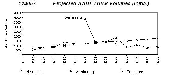
Truck Volumes–There were no large discrepancies between the historical and monitoring trucks volumes. The truck volume projection model–the model estimating the total annual number of trucks for each year since the highway was opened to traffic–fit the annual historical and monitoring truck volumes within a typical range of about ±50 percent. Outliers were permitted where it was felt that the historical or monitoring data were probably in error. An example of a truck volume projection model that contains an outlier is shown in figure 17.

Truck Classification–the distribution of trucks into the 13 FHWA vehicle classes appeared to be reasonable considering:

• The functional class of the highway. For example, it was expected that about 50 to 80 percent of all trucks on rural interstates would consist of five–axle single trailer trucks (vehicle Class 9).
• Monitoring truck class distribution obtained for different years. It was expected that the truck class distribution for the major truck classes such as Class 5 and Class 9 vehicles (table 1) would not vary by more than about ±25 percent from year to year (particularly on highways with daily truck volumes exceeding about 300 trucks).
• Relatively small number of unclassified vehicles. Typically, the number of unclassified vehicles did not exceed about 15 percent of all vehicles.

Figure 17. Projected AADT truck volumes for site 124057.

Axle Weights–The distribution of axle weights appeared to be reasonable considering:

• There was a basic correspondence between the truck class distribution and the truck axle load spectra. For example, for the sites with many two–axle trucks, the predominant component of the axle load spectra was expected to be single axles.
• There was at least one year for which axle load spectra were considered to be appropriate. Typical characteristics of acceptable axle load spectra are summarized in table 6, and included:
  • Single axles had a predominant peak at about 4,540 to 5,448 kg (10,000 to 12,000 lb), and a secondary peak (when warranted by the truck classification data indicating the presence of vehicles with single axles carrying payload) at about 7,264 to 8,172 kg (16,000 to 18,000 lb).
  • Tandem axles had the loaded peak at about 14,074 to 14,982 kg (31,000 to 33,000 lb) for agencies with the allowable axle weight for tandem axles of 15,436 kg (34,000 lb). The unloaded peak was about 3,178 to 5,448 kg (7,000 to 12,000 lb).
  • Triple axles had the peak at about 18,160 kg (40,000 lb), and their number was commensurable with the occurrence of six–and–more axle trucks. Based on the Bridge Gross Weight Formula, for the triple axle spacing exceeding 2.44 m (8 ft), the allowable axle weight is 19,068 kg (42,000 lb).^[13]
• If the axle load spectra were available for more than 2 years, the requirements for the peak axle weights to reach the specific ranges were relaxed because the base annual spectra were calculated as an average of all annual spectra that were considered acceptable.
• For agencies that provided apparently good estimates of historical truck volumes and TFs, the monitoring TFs were typically within ±50 percent of the historical TFs.

For a few sites, the quality of axle weight data was also evaluated by examining the distribution of gross vehicle weights (GVW) for Class 9 vehicles (5–axle single trailer trucks). The logic underlying the QC process utilizing the GVW distribution is that many Class 9 trucks operate either unloaded or loaded, and if loaded their GVW is close to the maximum allowable GVW of 36,320 kg (80,000 lb). Thus, a typical distribution of the GVW of Class 9 vehicles is expected to have two peaks, the first peak, associated with unloaded vehicles, at about 12,712 to 16,344 kg (28,000 to 36,000 lb), and the second peak, associated with loaded vehicles, at 31,780 to 35,412 kg (70,000 to 78,000 lb).

The reasons for not using GVW of Class 9 vehicles more extensively included:

• For sites where Class 9 vehicles predominate (for example on rural interstates and on other major rural highways), the plots of single and tandem axle load distributions are governed by the presence of the Class 9 vehicles already (and convey similar information as the GVW plots).
• For sites where Class 9 vehicles do not dominate (for example on some urban highways and minor rural roads), the knowledge of the GVW distribution of Class 9 vehicles is not critical for assessing the quality of axle weight data.
• The weights of the individual vehicles are not stored in the IMS database and the production of the GVW plots would require considerable additional analytical effort.

The use of the GWV distribution of Class 9 vehicles is recommended in the LTPP Traffic QC User's Guide as the basic QA process for the operation of WIM scales.^[12]

Regardless of the use of the GVW of Class 9 vehicles, there are fundamental differences between (a) the QA process using the GVW of Class 9 vehicles recommended by the user's guide and (b) the traffic data assessment process used to carry out traffic projection and the assignment of the projection confidence codes. The fundamental differences are in the timing, outcome, and length of the time period for which the data were assessed as outlined previously. It appears that the many axle load data stored in the IMS have not been subjected to the QC process recommended by the LTPP Traffic QC User's Guide.

Example of Assigning IA Code–The following example summarizes some considerations involved in assigning IA codes. Many considerations also apply to traffic data assessment and traffic projection activities done in unison with the assignment of projection confidence codes.

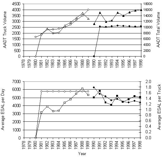
The appearance of annual axle load spectra shown in figure 13 was one reason the IA code was assigned to the traffic projections carried out for site 063042. The nine annual axle load spectra for this site (for 1990 to 1998, inclusive) show a consistent downward trend, illustrated by the plot of average ESALs per truck (figure 18).

According to figure 18, the average ESALs per truck gradually declined between 1990 and 1998 from 1.8 to about 1.3 per truck. However, because there has been a significant increase in truck volume at the same time, the total annual number of ESALs has remained relatively constant. The reason the decline appears to be real (not caused by a WIM scale calibration drift) is based on the observation that axle weights that are not sensitive to payload have remained relatively unchanged, whereas the weight of loaded axles has gradually declined. For example, the second peak of the single axle load spectra (top chart in figure 13) can be attributed principally to the steering axle of heavy trucks. The load on the steering axle of these trucks is relatively insensitive to the load carried and has remained substantially unchanged over recent years. Similarly, the first peak for tandem axles (middle chart in figure 13), which corresponds to unloaded tandem axles, has also remained unchanged. On the other hand, the second peak for tandem axles, corresponding to loaded payload–carrying tandem axles, gradually declined.

It is possible that the historical decline in axle weights reflected in the decline in ESALs per truck is the result of deregulation process of the motor carrier industry and the emergence of low–weight high–value freight.^[15]

063042 Annual Traffic Projection Sheet

Figure 18. Annual Traffic Projection Sheet for site 063042.

Additional considerations that lead to the assignment of the IA code included:

• Three well–defined peaks for annual load spectra for single axles (first part of figure 13). The first peak at about 1,816 kg (4,000 lb) corresponds to Class 5 vehicles (2–axle single unit trucks), the second peak at about 4,994 kg (11,000 lb) to steering axles of Class 9 vehicles, and the third peak corresponds to load axles of Class 9 vehicle consisting of a 3–axle single unit truck pulling a 2–axle trailer (a truck type common on some highways in California).
• Clearly defined and logical trend in historical and monitoring AADT truck volumes (first part of figure 18).
• Correspondence between historical and monitoring TFs (second part of figure 18).
• Relatively small number of triple axles that had been gradually increasing over the years.

Guidelines for Assigning IN Codes

The IN code means that the axle load projections were not carried out at this time because of lack of site–specific axle load data. For some sites, the IN code was assigned because there were no site–specific axle load data. For other sites, there were axle load data, but the data were questionable to the degree that it appeared probable that better traffic load estimates could be provided by using surrogate (regional or generic) axle load data rather than by using the available site–specific axle load data. However, for all sites with historical or monitoring truck volume data, but without axle weight data, annual truck volume projections were still carried out for all in–service years. The exceptions were four Specific Pavement Section (SPS)–8 sites (environmental sites with little or no truck traffic).

Because both truck volumes and axle load data were used for the projection of traffic loads, a site could be assigned the IN code due to inadequacies in: (a) truck volume data alone; (b) axle load data alone; or (c) the combination of truck volume and axle load data. However, the situations where the IN code was assigned primarily because of inadequacies in truck volume data were rare. The typical reason for assigning the IN code was the combination of truck volume and axle load data inadequacies, with the inadequacies in axle load data predominating.

The guidelines for assigning IN code do not enumerate all possible combinations of truck volume, truck distribution, and axle load data inadequacies. The principal consideration in assigning the IN code was the judgment whether the traffic projection using the available site–specific data would be likely to provide better results than could be obtained using surrogate traffic data.

Truck Volume–Typical problems encountered included large differences between historical and monitoring truck volumes and/or large variation in monitoring truck volumes, making the estimates of annual truck volumes unreliable.

Truck Classification–The truck distribution could exhibit any combination of the following problems:

• Unexpected truck distribution considering the highway functional type. For example, a higher percentage of four–or–less–axle single trailer trucks (class 8) than of five–axle single trailer trucks (class 9) on a rural interstate.
• Highly variable annual truck distributions, with no single annual distribution that could be identified as being correct or expected.
• A large number of unclassified vehicles, sometimes exceeding 50 percent.

Axle Weights–Conditions that characterized axle load spectra that were considered to be inadequate, and that were not used for the projection, included:

• Disjointed truck class distribution and axle load distribution data. For example, axle load spectra for single and tandem axles would appear as flat lines while the truck class distribution would indicate that the predominant truck type was Class 9.
• A large variation in annual axle load spectra, but without a year for which the annual axle load spectrum could be considered appropriate. For example, for a 4–lane highway, an annual tandem axle load spectrum would have only 10 percent of axles weighing more than 6,810 kg (15,000 lb) one year, whereas the next year 50 percent of tandem axles would be more than 15,463 kg (34,000 lb).
• Monitoring TFs appeared to be unreasonable judging by (a) historical TFs and (b) TFs obtained on similar sites. For example, a monitoring TF for an interstate would be less than 0.2, while the corresponding historical TF would be 1.2 (reported by an agency that provided historical TFs that have been, in general, in good agreement with monitoring TFs), and the monitoring TFs obtained for similar sites (for the same agency and the same pavement type) were in the range of 0.8 to 1.3.

Example of Assigning IN Code–The shape of the annual axle load spectra presented in figure 16 was the main reason the IN code was assigned to site 473104 and no axle load projections were done for this site. The annual axle load spectra shown in figure 16 exhibit considerable variation. For example, the 1992 TF was about 0.1, while the 1996 factor was about 4.0. Truck volume projections were still carried out and are shown in figure 19.

Guidelines for Assigning IQ Codes

The IQ code was assigned to sites with traffic data characteristics falling between IA and IN characteristics. In other words, the projected traffic loads were probably better than the estimates based entirely on surrogate axle load data but not as good as the IA results. Cumulative ESAL estimates were probably typically within ±100 percent of the actual ESALs.

Example of Assigning IQ Code–The assignment of IQ codes is illustrated using examples for sites 285805 (figure 8) and 124057 (figure 15).

The main reason for assigning the IQ code to site 285805 was inconsistencies in annual axle load spectra. The peak of single axle load spectra for all years was below 4,540 kg (10,000 lb) (figure 8), even though about 65 percent of all trucks were Class 9 trucks (figure 7). It was unclear whether the 1996 tandem axle load spectra were better than the spectra for the remaining years (1992 to 1995). The annual truck traffic projection model followed the trend set by the monitoring truck volumes (figure 6).

The shape of the annual axle load spectra for site 124057, presented in figure 15, was not the main reason the IQ code was assigned to this site. The 1991 and 1992 spectra appear to be reasonable even though their peaks for single axle loads at about 3,632 kg (8,000 lb) were lower than expected. The main reason was the uncertainty regarding the projection of truck volumes (see figure 17). According to figure 17, the initial truck volume projection was based on historical data and on estimated monitoring data only. The monitoring truck volumes show a decline between 1992 and 1998.

Concluding Remarks

The projection confidence codes are subjectively assigned indicators of the reliability of traffic load estimates. The codes may change if more data become available, or a different interpretation of the data is made. The initial codes may also change after the initial traffic projections are reviewed by the agencies. For example, the initial IQ code for site 285805 was changed to IA based on the review of the initial projection provided by a representative of the Mississippi DOT. The review confirmed the legitimacy of 1996 axle load spectra (figure 8) and the appropriateness of the initial truck volume projection (figure 6).

Computation of Annual Axle Load Spectra

The computation of annual axle load spectra was carried out using a procedure outlined by equation 1. In addition, for QC purposes, annual ESALs and cumulative ESALs were also calculated using projected axle load spectra and compared with historical and monitoring ESALs, as shown in figure 10.