U.S. Department of Transportation
Federal Highway Administration
1200 New Jersey Avenue, SE
Washington, DC 20590
202-366-4000
Federal Highway Administration Research and Technology
Coordinating, Developing, and Delivering Highway Transportation Innovations
 |
| This report is an archived publication and may contain dated technical, contact, and link information |
| breadcrumb |
Publication Number: FHWA-HRT-04-079
Date: July 2006 |
|||||||||||||||||||||||||||||||||||||||||||||||||||||||||||||||||||||||||||||||||||||||||||||||||||||||||||||||||||||||||||||||||||||||||||||||||||||||||||||||||||||||||||||||||||||||||||||||||||||||||||||||||||||||||||||||||||||||||||||||||||||||||||||||||||||||||||||||||||||||||||||||||||||||||||||||||||||||||||||||||||||||||||||||||||||||||||||||||||||||||||||||||||||||||||||||||||||||||||||||||||||||||||||||||||||||||||||||||||||||||||||||||||||||||||||||||||||||||||||||||||||||||||||||||||||||||||||||||||||||||||||||||||||||||||||||||||||||||||||||||||||||||||||||||||||||||||||||||||||||||||||||||||||||||||||||||||||||||||||||||||||||||||||||||||||||||||||||||||||||||||||||||||||||||||||||||||||||||||||||||||||||||||||||||||||||||||||||||||||||||||||||||||||||||||||||||||||||||||||||||||||||||||||||||||||||||||||||||||||||||||||||||||||||||||||||||||||||||||||||||||||||||||||||||||||||||||||||||||||||||||||||||||||||||||||||||||||||||||||||||||||||||||||||||||||||||||||||||||||||
Seasonal Variations in The Moduli of Unbound Pavement LayersChapter 5: Prediction of Backcalculation Pavement Layer ModuliINTRODUCTIONThis chapter discusses the development of relationships to predict backcalculated moduli for unbound pavement layers. The models discussed address the effects of both moisture condition and stress state on the moduli of these layers in the nonfrozen condition. The backcalculated pavement layer moduli used in this work are those from the LTPP database that remained in the working data set after the review process discussed under Evaluation of Backcalculated Layer Moduli" in Chapter 3. The stress parameters considered were computed by the author, as discussed under "STRESS PARAMETERS" in Chapter 3. Input to these computations included the backcalculated pavement layer moduli, the layer thickness, and Poisson’s ratios used in the backcalculation process, and (in the case of overburden stresses) the layer densities, daily mean layer moisture contents, and water table depth data from the LTPP database. The moisture contents considered in this work were daily mean values computed from the TDR-based moisture content data for each pavement layer (see "Moisture Parameters," Chapter 3). The sources of variation reflected in the data set included variations with FWD load (by virtue of the use of multiple FWD load levels at each test date and time), point-to point variations, within-day variations (by virtue of repeated test cycles within a day), and longer-term variations (through use of data for multiple test dates). EXPLORATION OF RELATIONSHIPS BETWEEN BACKCALCULATED MODULI AND EXPLANATORY VARIABLESAttempts to develop predictive models for backcalculated pavement layer moduli were preceded by examination of a series of correlation matrices exploring the relationship between the backcalculated layer moduli, stress state variables, and the TDR-monitored moisture content. The variables considered in these matrices are: Log(E); the mean volumetric moisture content (Vm) for the layer; the applied FWD load (P); the radial load stress (sr); the bulk and octahedral shear stresses due to load and overburden (?, and t); log(?/Pa); and log(t/Pa+1). Radial overburden was computed assuming k0 = 1.0 in all cases. The stress parameters were computed for points directly beneath the center of the loaded area, and at depths of one-quarter-depth, mid-layer, and three-quarters-depth within the finite layers, and at 0.1, 0.2, and 0.3 m (3.9, 7.9, and 11.8 inches) beneath the layer interface for semi-infinite subgrade layers. Pertinent observations drawn from these correlation matrices are as follows. The observed correlation between modulus and moisture content is summarized in Table 32.For 53 percent of the pavement layers, the correlation between modulus and moisture content is negative, indicating that increases in moisture are associated with decreases in modulus. The opposite is true for the remaining 47 percent of the pavement layers. The strength of the observed correlation, whether positive or negative, varies tremendously-from essentially zero, to 0.73 on the positive side, and 0.99 on the negative side. Both positive and negative correlations are observed for all of the soil classes represented in the data set, and all layers in the pavement structure. The prevalence of positive correlations is contrary to expectations. Table 33 summarizes the observed correlation between modulus and applied FWD load. As was the case for the moisture-modulus correlations, the strength of the correlations between modulus and applied FWD load varies considerably, with values spanning the range from - 0.80 to 0.92. For the majority of the base layers, the expected positive correlation, implying increasing modulus with increasing FWD load, is observed. The direction of the observed correlations is less consistent for the deeper layers. The prevalence of negative correlations (implying decreasing modulus with increasing FWD load) for granular layers is contrary to expectations, and inconsistent with the findings presented in Chapter 3 that were based on paired comparisons of moduli for different load levels with all other factors constant. For this reason, it is reasonable to attribute the unexpected frequency of negative correlations to the confounding influence of variations in moisture and other factors with time.
In reviewing the correlation matrices, it was found that the backcalculated modulus is often less strongly correlated with moisture than with one or more of the stress parameters considered. This is true for all of the base layers, 82 percent of the subbase/upper subgrade (layer 3) layers, and 80 percent of the subgrade/lower subgrade (layer 4) layers. The exceptions occurred for the upper subgrade layer at section 131005 (A-4), the subgrade at section 251002 (an A-3 soil), both the subbase and subgrade layers at section 831801 (A-2-6 and A-2-4, respectively) and both the subbase and subgrade at section 241634(both A-4). For 63 percent of the layers, the backcalculated modulus is more strongly correlated with the radial load stress computed at one or more depths than it is with either moisture, or the bulk or octahedral shear stresses.
The relative strength of the observed correlations between log En and the bulk and octahedral shear stress parameters is summarized in Table 34. This information is inconsistent with expectations based on laboratory Mr test results. Lab data typically indicate that bulk stress is the more important predictor of modulus for granular materials, whereas the correlations for the backcalculated moduli indicate that the octahedral shear stress is often the more important predictor for both granular and fine-grained materials. Conversely, based on laboratory data, one would expect the octahedral shear stress to be the more important predictor for the finegrained soils, but the data in Table 34 indicate that this is not always the case, as A-4 soils are among those for which the backcalculated modulus is more strongly correlated with the bulk stress than with the octahedral shear stress.
The sign (positive or negative) of the observed correlations between backcalculated modulus and the bulk and octahedral shear stress parameters is summarized in Table 35. Based on laboratory test experience, positive correlation (corresponding to increasing modulus with increasing stress) between modulus and the bulk stress is expected for all granular layers. For the backcalculated moduli, both positive and negative correlations with bulk stress occur. The relative frequency of occurrence of positive and negative correlations varies with the layer and the stress computation depth considered. Negative correlations (indicative of stresssoftening behavior) are expected for the fine-grained soils. Again, some observed correlations for the backcalculated layer moduli are consistent with this expectation, while others are not. The correlation matrices were reviewed to identify the depth at which the computed stress parameters were most strongly correlated with the backcalculated moduli. The findings of this review are summarized in Table 36. More often than not, the correlations for the one-quarterdepth and three-quarters-depth stress computation points are stronger than those for the midlayer stresses. The frequencies with which the strongest correlations between E and bulk stress are observed at one-quarter-depth and three-quarters-depth in the layer are similar. The strongest correlations with octahedral shear stress occur most often at three-quarters-depth within the layer for the finite layers, and at 0.1-m below the layer interface for the semiinfinite subgrade layers. Between-depth differences in the strength of the observed correlation range from zero (for t and log t at section 351112, layer 4) to more than 0.60 (for log ? at section 040113, layer 2).
The relationship between variations in backcalculated modulus and moisture was also examined by looking at the ratio ?E/?Vw, where ?E and ?Vw are the change in modulus and moisture relative to a reference condition. The reference condition that was used was the earliest available modulus/moisture observation for each nominal FWD load level for a particular test section and layer. Summary values by layer type are presented in Table 37. Pertinent observations follow the table.
The ratio ?E/?Vw is highly variable, with a range of -4,590 to 7,860 kPa (-666 to 1140 psi) per 1-percent change in moisture content. Both positive and negative values of the ratio are observed for 92 percent of the individual layer and load level combinations. Thus, in most cases, both increases and decreases in backcalculated modulus are associated with increases in mean layer moisture content. Exceptions to this general rule occur on a consistent basis (across all FWD load levels) for the subgrade layer at section 041024 (Arizona), the subgrade layer at section 081053 (Colorado), and the base layer at section 906405 (Saskatchewan). However, in all of these cases, the number of observations considered is small, so it is not clear that these layers are truly exceptional in this regard. The mean values of the ratio ?E/?Vw for individual layers and load levels vary in the range of -403 to 1,089 kPa (-58 to 158 psi) per one percent change in moisture content, with the overall mean value being -4. The coefficient of variation (COV) observed for individual combinations of layer and load level varies from a low of 13 percent for the base (layer 2) at section 041024 (Arizona), to a high of more than 20,000 percent for the upper subgrade (layer 3) at section 231026 (Maine), with the overall average COV being 761 percent. In many cases, both the mean ratio and the extent of variation therein vary between load levels, but universally applicable trends are not evident. In looking at the statistics on a layer-type basis, it may be observed that the mean ratio for the base layers decreases with increasing load on a consistent basis. However, the standard deviations associated with the mean values are so large in comparison to the means that this trend in not particularly meaningful. The COV for the base layer group increases with increasing load, from a low of 2,605 percent for the nominal 27-kN (6,070 lbf) load to a high of 111,707 percent for the 71-kN (15,961 lbf) load level. In contrast, the subbase layer values for the 40-, 53-, and 71-kN (8,992-, 11,915-, and 15,961-lbf) load levels are remarkably similar. Overall, the high degree of variability in the ratio ?E/?Vw suggests that factors other than moisture (e.g., stress conditions) may be important to explaining the observed variations. In summary, plots of modulus versus moisture, correlation matrices, and the ratio ?E/?Vw were examined with the following findings.
Together, these observations suggest that moisture is not always the primary driver of seasonal variations in backcalculated pavement layer moduli. MODELS OF THE FORM E/Pa=k1?/Pak2(t/Pa+1)k3Initial efforts to develop predictive models for backcalculated pavement layer moduli focused on the model form presented as Equation 26,
with k1 taken to be k0*10c1Vw.(Vw is the volumetric moisture content, expressed as a percent;ci and ki are regression constants; and all other variables are as previously defined.) This model form was selected to be consistent with the constitutive model to be used for unbound materials in the 2002 Guide for Design of New and Rehabilitated Pavement Structures that is currently under development. Note that it is a variant of Equation 11, in which k6 is taken to be zero, and k7 is assumed to be 1. This model will henceforth be referred to as Model 1. Both load-induced and overburden stresses were included in the computation of the stress parameters. The horizontal overburden stresses were computed using k0 values of 0.7 and 0.5 for the base and subbase/subgrade layers, respectively. Temporal variations in overburden due to variations in mean layer moisture content were considered in the calculation (although it is likely that the impact of this is very small). The stresses considered were those computed at a point directly beneath the center of the loaded area at 0.75-depth within each finite layer, and at 0.3 m below the layer interface for each semi-infinite layer. For the purposes of the regression modeling, Model 1 was transformed by taking the log of both sides of Equation 26, so that standard multiple regression could be used to derive the regression coefficients. The transformed model (with the moisture term explicitly included) is given in Equation 27.
The multiple regression results obtained for individual pavement layers are presented in Table 73 in Appendix E: Multiple Regression Results for Individual Pavement Layers. From a standpoint of goodness of fit, as judged by the fraction of variance explained by the model (R2) and the standard error ratio (Se/Sy) computed for log E, as well as the bias and standard error ratio for E, many (but not all) models are quite good. However, although most of the materials in question are granular, the majority of the k2 values are negative, indicating that the modulus decreases with increasing bulk stress (i.e., "stress softening"). This is inconsistent with the stress-hardening behavior typically exhibited by such materials in the laboratory and the load-hardening behavior of the pavement layers discussed previously. Most positive values for k3 are similarly inconsistent with laboratory test findings. The signs of both k2 and k3, however, are consistent with correlations discussed previously. Several alternative approaches to computation of the stress parameters were explored in an attempt to produce models with regression coefficients that are more consistent with laboratory test results. Those alternatives are summarized in Table 38. The factors that were varied were the assumed values for K0 used in computing the horizontal overburden stresses, and whether overburden stresses were or were not included in the computation of the stress parameters. The K0 values were varied to explore the possibility that the poor agreement between the regression results obtained with backcalculated layer moduli and laboratory test results came about as a result of incorrect assumed values for K0 (the true values being unknown). The use of only the load-induced stresses for one or both of the stress parameters was pursued to explore the possibility that overburden stresses are not important to the observed variations in backcalculated pavement layer moduli. Stresses computed at threequarters-depth in the pavement layer were used in this analysis, and, k1 was taken to be constant (i.e., not a function of the volumetric moisture content). Thus, the transformed model form used in the multiple regression to obtain the model coefficients is:
The results obtained for the alternative stress computation assumptions are presented in Table 74 through Table 80 in Appendix E: Multiple Regression Results for Individual Pavement Layers. The regression coefficients for these models are summarized by soil class in Table 39. Only those regression results meeting a minimum goodness of fit standard of R2 =0.60 (in log space) were included in the preparation of this summary. A complete evaluation of the adequacy of these regression models was not undertaken, as the goal of achieving coefficients consistent with laboratory test results was not achieved.
The results obtained with all stress data sets identified in Table 38 are qualitatively similar to those obtained in the initial effort. The majority of the k2 values are negative for both the granular and fine-grained materials, and the k3 values are typically positive. While the k1 values are similar in magnitude to the laboratory resilient modulus coefficients reported by Von Quintus and Killingsworth (see Table 9), the k2 and k3 values differ in both magnitude and sign.[5] For example, Von Quintus and Killingsworth report k1 values in the range of 250 to 2,323; k2 values in the range of -0.18 to 1.07; and k3 values in the range of -0.33 to 0.61 for base materials, while the corresponding Table 39 values for A-1-a soils vary in the ranges of 59 to 2078; -9.21 to -0.07; and -0.41 to 12.8, respectively. None of the options considered resolves the inconsistency with laboratory test results. Subsequent efforts to identify an alternative radial location for stress computation that would yield acceptable results from a standpoint of both goodness of fit and consistency with laboratory test results were similarly unsuccessful.
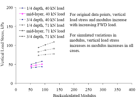
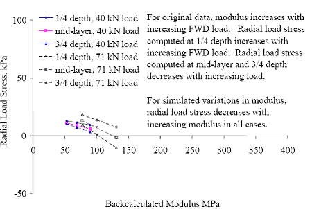
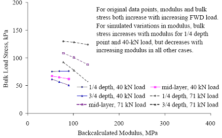
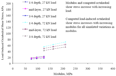
FACTORS CONTRIBUTING TO DIFFERENCES BETWEEN LABORATORY AND FIELD-BASED CONSTITUTIVE MODEL COEFFICIENTSIn comparing backcalculated pavement layer moduli with laboratory resilient moduli, it is important to keep in mind what is being compared. As discussed previously, the laboratory test result is appropriately termed a material property-a measurable characteristic of the material. In contrast, the backcalculated layer modulus is more correctly thought of as a parameter-an estimate of the "average" material characteristic for the pavement layer, which does not fully account for spatial variations in stress state (and thus, stiffness). Furthermore, the interpretation process used to obtain the estimate is based on theory that approximates, but does not match, reality. Key theoretical assumptions that are violated to one degree or another are the assumptions of homogeneity, isotropy, and linearity. In the interpretation of laboratory resilient modulus test data we have measurements of the confining pressure and the cyclic axial load from which the major and minor principal stresses applied to the test sample are computed. For the most common laboratory situation, the radial and vertical stresses are: (1) always compressive; (2) independent of each other; (3) independent of the modulus of the material; and (4) applicable to the sample as a whole. In contrast, when looking at backcalculated layer moduli, one must compute the applicable overburden and load-induced stresses. By virtue of the theory used (linear layered-elastic theory), the computed stresses are: (1) sometimes tensile; (2) not independent of each other; (3) not independent of the modulus of the material, and (4) applicable to a particular point in the pavement layer, rather than a well-defined volume of soil. Furthermore, it is probable that the location of the point at which the computed stress parameters are most representative of thelayer as a whole varies not only from one pavement to another, but from point to point and day to day (if not hour to hour) by virtue of spatial and temporal variations in the pavement layer properties. The stress parameters used in modeling the stress sensitivity of the backcalculated moduli are themselves a function of the backcalculated layer moduli. This has some important implications, chief among them the potential for the radial load stress to decrease as the modulus increases, with all other factors held constant. In Figure 32 and Figure 33, data for two different FWD load levels from a single FWD drop sequence are used to illustrate the impact of this possible occurrence on the relationship between backcalculated moduli and computed stress parameters. For each set of backcalculated layer moduli, stresses were computed for the original set of backcalculated layer moduli, and for two modified data sets. In one version, the modulus for one (and only one) layer was multiplied by 1.3. In the other, the modulus for the same layer was divided by 1.3. The simulated variations (outer points in each curve) illustrate how the computed stresses vary with the modulus of one layer, when all other factors are held constant, while the actual data points (which appear as the center point in each curve) show the overall impact of FWD load level on the stresses and moduli for the layer under consideration (including load-related variations in the moduli of other layers. The stresses were computed for a point directly beneath the center of the applied load. Three different computation depths were considered for each layer, corresponding to one-quarter-depth, midlayer, and three-quarters-depth. In Figure 32, the observed variation in computed vertical load stress is reasonably consistent with the laboratory test situation for granular materials-a direct relationship between modulus and vertical stress. However, the same cannot be said for the radial load stress, illustrated in Figure 33. For two of the three stress computation depths, there is an inverse relationship between the radial load stress computed for the original data (center point on curves) and the backcalculated modulus and FWD load. An inverse relationship between modulus and radial load stress also occurs for all three stress computation depths considered for the simulated variations in modulus. Also, note that some computed radial stresses are negative (tensile). The impact of these variations on the relationship between backcalculated modulus and the computed load-induced bulk and octahedral shear stresses is illustrated in Figures 34 and 35. In this case, the original data points all show an increase in both modulus and bulk load stress with increasing FWD load, while both direct and inverse relationships between modulus and bulk stress occur for the simulated variations. The computed octahedral shear stresses consistently increase with increasing modulus. The trends shown in these figures do not represent universal truth. Rather, they illustrate that use of linear layered-elastic theory to backcalculate moduli and compute the associated loadinduced stresses can result in inverse relationships between backcalculated layer moduli and bulk stress, even though the expected load-hardening behavior is observed in the backcalculated moduli. This situation is compounded by the fact that the computed radial load stress may also be negative. The varying trends in the computed radial load stress, and the occurrence of negative values, manifest themselves in varying trends in the computed bulk stress. The impact of the varying radial load stress trends and tensile radial load stresses on the computed octahedral shear stress is less obvious (but no less important), by virtue of the mathematical definition of that parameter. Figure 32. Vertical load stress versus modulus, section 040113 A-1-a base layer
Figure 33. Radial load stress versus modulus, section 040113 A-1-a base layer
Figure 34. Bulk load stress versus modulus, section 040113 A-1-a base layer
Figure 35. Load-induced octahedral shear stress versus modulus,section 040113 A-1-a base layer
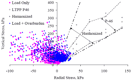
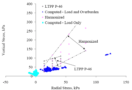
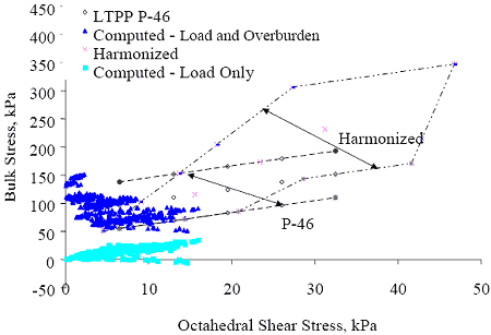
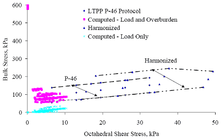
The vertical and radial stresses (sv and sr) computed for the backcalculated moduli are compared with those for two laboratory resilient modulus test protocols in Figure 36 to Figure 38. The test protocols considered are the LTPP P-46 protocol,[80] and the proposed "harmonized" protocol developed under NCHRP project 1-28A.[45] The stresses plotted in these figures were computed for points directly below the center of the loaded area, at threefourths- depth within the pavement layer, with k0 = 1.0, for the first set of backcalculated moduli for each test date and FWD load level. Plots prepared with stresses computed at onequarter- depth or mid-layer are qualitatively similar. While the stresses plotted in these figures do not represent universal truth, they are representative of the data set used in this investigation (see Table 18 and Table 19), and serve to illustrate the conditions that can exist when linear layered-elastic theory is used to backcalculate pavement layer moduli andcompute the load-induced stresses in the pavement structure. Figure 36. Comparison of radial and vertical stress components for granular base and subbase layers
The principal stresses defined in the two laboratory test protocols are similar, though those for the harmonized protocol are more extensive. While some computed stress data points for the base and subbase materials (Figure 36) fall within the bounds defined by the laboratory test protocols, many do not. Of particular significance is that a large fraction of the computed radial load stresses are negative, particularly for the base layers. Figure 37. Comparison of radial and vertical stress components for coarse-grained subgrade layers
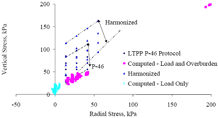
Figure 38. Comparison of radial and vertical stress components for fine-grained subgrade layers
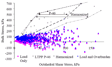
Computed subgrade stresses illustrated in Figures 37 and 38 are more similar to those for the laboratory stresses than those for the base and subgrade layers, but many data points fall outside the envelopes defined by the laboratory test protocols. Negative computed radial stresses are again prevalent. The corresponding bulk and octahedral shear stresses are shown in Figure 39 to Figure 41. As one would expect given the relationships observed in Figure 36 to Figure 38, the stress states computed from the backcalculated layer moduli bear little resemblance to those for either laboratory protocol. (Note that the scales used in these figures are such that the higher stress states for the harmonized protocol are not shown.) Thus, it is reasonable to conclude that the model coefficients derived for the backcalculated layer moduli differ from those obtained for laboratory resilient modulus test results because the stress states computed for the backcalculated moduli using layered-elastic theory are not directly analogous to the lab stress states. Therefore, it is impossible to derive constitutive model coefficients that are compatible with laboratory test data from the backcalculated layer moduli. Figure 39. Comparison of bulk and octahedral shear stresses for granular base and subbase layers
Figure 40. Comparison of bulk and octahedral shear stresses for coarse-grained subgrade layers
Figure 41. Comparison of bulk and octahedral shear stresses for fine-grained subgrade layers
In light of these observations, it might be argued that the solution to the observed discrepancies is to abandon the use of linear layered-elastic theory in the interpretation of pavement deflection data. However, while nonlinear backcalculation is an essential long-term goal, abandoning backcalculation based on linear layered-elastic theory is not a practical solution at this time. Given the current state of the art, it is likely that backcalculation based on linear layered-elastic theory (with or without adaptations to consider the stress sensitivity of materials in an approximate fashion) will remain the best available technology applicable in routine practice for at least the next several years. Thus, it is appropriate to pursue models to predict the observed variations in layer moduli backcalculated using linear layered-elastic theory, even though the model coefficients obtained are not directly analogous to those derived from laboratory test results for the same or similar materials. ALTERNATIVE MODEL FORMSIndividual Pavement Layer ModelsGiven the differences between the computed stresses based on linear layered elastic theory and laboratory stress states discussed in the preceding section, it is appropriate to consider possible modifications of the constitutive model form to improve the predictive capability for the backcalculated layer moduli. The primary modification considered was the substitution of a semi-log form for the bulk stress term in the model, as shown in Equation 29 (Model 2).
Use of the semi-log form for the bulk stress term enables straightforward consideration of negative computed bulk stress terms. This rationale does not apply to the octahedral shear stress term, as it cannot be negative, so the log-log form was retained for the octahedral shear stress term, to maximize consistency with the original model form. Two variations on the model form were considered: model 2A, in which k1 was taken to be a function of the volumetric moisture content, and model 2B, in which all three regression parameters were treated as being (potentially) a function of the volumetric moisture content. These variations are presented as Equations 30 and 31, respectively.
The models were fitted using multiple regression applied to the log-transformed models, as presented in Table 40. In the equations in Table 40, the c0’= log c0. The computation of the stress parameters considered in these models differed from that for Model 1 in one respect,the value of K0 used in the computation of the radial overburden stresses. For these models,K0 was taken to be 1.0 for all layers.
Regression results obtained for individual layers using 2A and 2B are presented in Table 81 through Table 82 of Appendix E: Multiple Regression Results for Individual Pavement Layers.The regression coefficients obtained for all four models are summarized in Table 41.
The regression coefficients obtained for both equations appear to be rational in the context of linear layered-elastic backcalculated moduli and computed stresses for the majority of the pavement layers considered. (They would not be considered rational in the context of traditional laboratory resilient modulus test experience.) In this context, the traditional interpretation that negative k2 values are associated with stress-softening behavior is not really applicable, because the relative importance of the bulk and octahedral shear stress terms is often the reverse of what is seen in the laboratory, due to the particulars of linear layeredelastic analysis. Despite the negative k2 values, the models predict increasing modulus with increasing FWD load for the granular layers. While the majority of the model coefficients are rational (in the context of linear layeredelastic analysis), there are several notable exceptions. For example, the c0 values for all the models for section 831801 layer 3 for both equations are very high. The goodness of fit statistics for the section 831801 layer 3 models are very good, but the sample size is very small, so the applicability of this model is limited. The goodness of fit statistics for Models 1, 2A, and 2B are compared on a layer-by-layer basis in Table 83 of Appendix E: Multiple Regression Results for Individual Pavement Layers, and summarized in Table 42. In some instances, the number of observations considered in the regression varied between Model 1 (n1) and the other equations (n2), by virtue of the presence of negative bulk stresses in the data sets. This was the case for 11 of the 59 layers considered. In a few instances, the number of observations excluded due to negative bulk stresses approached the total number of observations available. In two cases, the exclusion of negative bulk stress observations made it impossible to complete the regression for Model 1, due to small sample sizes.
In most cases, providing for the possibility that all three k-coefficients vary with moisture content yields a better fit of the data (most often reflected in a reduced standard error ratio (Se/Sy)) than the assumption that only k1 is a function of moisture content. In some cases (e.g., layer 4 for section 040114), the difference is negligible (zero percent change in bias, and standard error ratio changed by less than 0.01), and in others it is more substantial (e.g., layer 4 for section 251002, where the standard error ratio was reduced from 0.96 to 0.38). The regression results were characterized as fully acceptable if the standard error ratio, Se/Sy, computed for Ep (as opposed to log(Ep)) was less than 0.5, and the absolute value of the bias was less than 2 percent. The results were characterized as unacceptable if the standard error ratio was greater than 0.85, or the absolute bias was greater than 5 percent. Results meeting neither set of criteria were characterized as marginal. Based on these criteria, all model forms considered yielded results that were at least marginally acceptable (from a standpoint of goodness of fit) for 61 percent of the pavement layers. Of 59 pavement layers considered, the regression results were unacceptable for 2, both subgrade layers, and 17 for which all model forms yielded fully acceptable results. The regression modeling was most successful for the base layers, and least successful for the semi-infinite subgrade layers. This discrepancy in the relative rate of success is consistent with the assumption that the true modulus of some of the semi-infinite subgrade layers is relatively constant with time and FWD load, such that the observed variation is primarily due to random error in the deflection testing and backcalculation process. Model 2 is better suited to modeling the variations in pavement layer moduli backcalculated using linear layered-elastic theory. The rationale underlying this judgment is as follows:
Furthermore, for 58 percent of the pavement layers, the standard error ratio for Model 2B is somewhat better than for Model 2A; consideration of the potential for moisture to affect all three k coefficients thus is recommended. It must be recognized that this recommendation applies only to layer moduli backcalculated using linear layered-elastic theory. No assessment of the applicability of the model form to laboratory resilient modulus test data has been undertaken. Soil Class ModelsThe regression models discussed in the preceding sections of this chapter were each derived from the data from a single pavement layer at a particular test section. In the interest of obtaining more broadly applicable models, the working data set of moduli, stress, and moisture parameters was subdivided by soil class and layer extent (i.e., whether the layer was finite or semi-infinite in depth). Multiple regression was used to fit the data for each subset to Model 2B, and several variations on Model 2 including material parameters, in addition to stress parameters and moisture content. The model forms considered for the coefficients k1, k2, and k3 are presented in Table 44. The materials data used in the models are presented in Appendix D:Materials Data Used In Development of E Predictive Models. Density and plasticity index are presented in Table 70, while gradation information is provided in Table 71. The resulting models are presented in Table 43. It is notable that the predictive capability of the soil class models (with or without material parameters) is often (but not always) better for the semi-infinite subgrade layers than it is for the soil classes most often found in the base and subbase layers-the opposite of what was observed for the individual layer models. Factors that may contribute to the observed discrepancy are as follows.
Differences in the number of sections (and therefore, the array of soils) considered in the model development may also contribute to the observed differences. The issue of the number of soils represented in the data sets on which these models are based is an important one, as the applicability of models based on data for only a few soils is limited; application of the models to the soil class in general thus is not appropriate.
Development of more general models-i.e., models applicable to all coarse-grained or all fine-grained soils-was attempted, but was not successful. SUMMARYRegression models to predict backcalculated pavement layer modulus as a function of stress state, moisture content, and (for the soil class models) material parameters were developed. In developing these models, regression coefficients derived for layer moduli backcalculated using linear layered elastic theory were found to be inconsistent with those obtained for laboratory test results for the same constitutive model form and similar materials. In particular, the sign of the k2 parameter for the backcalculated moduli for granular materials was consistently negative, when positive values are expected. The reasons for this discrepancy were explored, with the finding that the stress states and the relationships between the stress parameters computed for the backcalculated moduli and those typically used in laboratory testing are dissimilar. Key factors contributing to the dissimilarity include the lack of independence between the backcalculated moduli and the (computed) stress parameters used in the model development, and the potential for tensile computed stresses. Development of empirical models to predict layer moduli derived using linear layered-elastic theory was pursued to facilitate consideration of seasonal variations pending the development of improved backcalculation procedures. Model 2, which is restated below, is recommended for use in modeling the stress sensitivity of layer moduli backcalculated using linear layered elastic theory. It is further recommended that Model 2B be used to consider the combined effects of stress and moisture on linear elastic backcalculated pavement layer moduli.
|
|||||||||||||||||||||||||||||||||||||||||||||||||||||||||||||||||||||||||||||||||||||||||||||||||||||||||||||||||||||||||||||||||||||||||||||||||||||||||||||||||||||||||||||||||||||||||||||||||||||||||||||||||||||||||||||||||||||||||||||||||||||||||||||||||||||||||||||||||||||||||||||||||||||||||||||||||||||||||||||||||||||||||||||||||||||||||||||||||||||||||||||||||||||||||||||||||||||||||||||||||||||||||||||||||||||||||||||||||||||||||||||||||||||||||||||||||||||||||||||||||||||||||||||||||||||||||||||||||||||||||||||||||||||||||||||||||||||||||||||||||||||||||||||||||||||||||||||||||||||||||||||||||||||||||||||||||||||||||||||||||||||||||||||||||||||||||||||||||||||||||||||||||||||||||||||||||||||||||||||||||||||||||||||||||||||||||||||||||||||||||||||||||||||||||||||||||||||||||||||||||||||||||||||||||||||||||||||||||||||||||||||||||||||||||||||||||||||||||||||||||||||||||||||||||||||||||||||||||||||||||||||||||||||||||||||||||||||||||||||||||||||||||||||||||||||||||||||||||||||||