U.S. Department of Transportation
Federal Highway Administration
1200 New Jersey Avenue, SE
Washington, DC 20590
202-366-4000
Federal Highway Administration Research and Technology
Coordinating, Developing, and Delivering Highway Transportation Innovations
| REPORT |
| This report is an archived publication and may contain dated technical, contact, and link information |
|
| Publication Number: FHWA-HRT-14-092 Date: February 2015 |
Publication Number: FHWA-HRT-14-092 Date: February 2015 |
The objective of this chapter is to introduce the methodology adopted to develop the LTPP AFM algorithm to detect JPCP transverse joint locations and to determine faulting at each of the detected joints. The procedure consists of the following five tasks:
The ERD at the University of Michigan Transportation Research Institute developed a file format with an ERD extension to facilitate automated plotting of simulation data, experimentally measured data, and data from various analysis programs. The LTPP profile data are presented in an ERD text file with profile information in two parts, the header and the data. The header portion of the ERD file consists of a series of conventional American Standard Code for Information Interchange text lines. These lines contain information used by post-processing tools to read the numerical data such as start and end locations of the survey, speed of the vehicle, sampling interval, date, and time. The data portion of the ERD file contains numbers organized into columns and rows. There are three columns: the left and right wheelpath profiles, and the center of the lane profile. The LTPP regional support contractors collect a minimum of five profile runs/files on each LTPP test section of 152.4 m in length. If more are needed, then they can collect up to a maximum of nine profile runs/files. Information for the five most representative profile runs/files that pass the ProQual quality check is included in the LTPP PPDB. This study used these five profile runs/files for computing JPCP joint faulting.
This study used MATLAB® software to process and analyze LTPP profile data. The data portion of the profile ERD file was loaded into the MATLAB® program using MATLAB®'s import function. The LTPP test sections are 152.4 m in length. LTPP profile data are collected for the entire length. A new "distance" column was created using the profile sampling interval (25 mm) information from the header portion of the ERD file.
Filtering is a process of applying a mathematical transformation to true profile data to remove redundant noise. It is almost always necessary to filter the sequence of numbers that makes up the profile and to view different types of profile features. Many filters exist. A moving average filter was selected, and both smoothing and anti-smoothing filters are applied in this study.
The moving average filter uses the average of several adjacent profile elevation points to replace each profile elevation point. In this study, a 300-mm (12 data points) moving average filter was applied. For a profile p that has been sampled at interval ΔX, a moving average smoothing filter is defined by the summation in figure 2.(5)

Figure 2 . Equation. Moving average smoothing filter.
Where:
Pfl is the smoothed profile (also called a low-pass filtered profile).
B is the base length of the moving average.
N is the number of samples included in the summation.
MATLAB®'s built-in moving average filter function was used to filter the true profile. Anti-smoothing filtering, also called high-pass filtering, is a process of subtracting the smoothed profile from the true/original road profile. The choice of base length for an anti-smoothing filter is important to be able to show either very short-duration bumps or long deviations in the profile elevation. A larger anti-smoothing filter base length eliminates small deviations. To detect transverse joints using profile data, it is important to apply an anti-smoothing filter with a smaller base length. Figure 3 and figure 4 show two anti-smoothed filter profiles with different anti-smoothing base lengths.
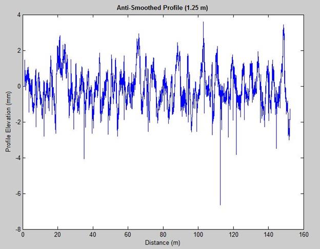
Figure 3 . Graph. Anti-smoothed profile with 1.25-m base length.
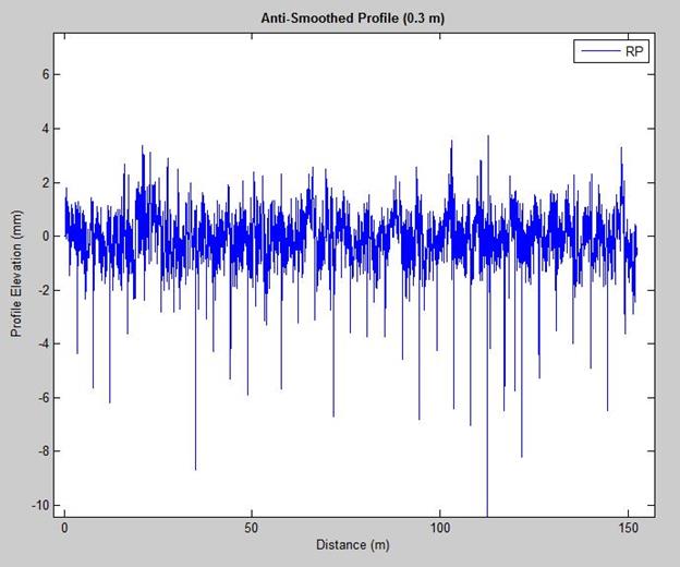
Figure 4 . Graph. Anti-smoothed profile with 0.3-m base length.
Figure 3 and figure 4 show that the anti-smoothed profile with a smaller base length (0.3 m) displays profile deviations (joints/cracks) more clearly compared with the anti-smoothed profile with a base length of 1.25 m.
Once smoothing and anti-smoothing filters are applied, the next step is to normalize the anti-smoothed profile with the root-mean-square (RMS) value. The RMS value provides the magnitude of the elevation profile and facilitates an automated search for the deepest dips or valleys.
The RMS value of a vector, X, is defined in figure 5 with the summation performed along the specified dimension.
After filtering a longitudinal profile for two wheelpaths (e.g., left and right wheelpaths) and a center of the lane profile, MATLAB®'s Peakdet algorithm, developed by Eli Billauer, is used, along with the moving window method, to detect the valleys.(16) The algorithm also cross-checks the detected valleys of one wheelpath against the other and against the center lane profile to detect a transverse joint (true joint on JPCP) and eliminate or minimize false positives (other than a true joint on JPCP). A peak is the highest point between valleys. Peakdet looks for the highest point around which there are points lower by Δ (positive value, for example, of 1 or 2) on both sides. A similar peak and valley detection algorithm was reported by Nazef et al.(10) Valleys in longitudinal road profile data collected on JPCP represent either potential joints or cracks. This study focuses on valleys that are transverse joints. Six steps describe how the Peakdet algorithm in MATLAB® detects peaks and valleys in a road elevation profile.
Step 1: Initialize the current elevation point (CEP) at V(i) and current elevation position (CEPos) at X(i) at the first point (i equals 1) in an elevation profile. For illustration, a moving window width of 4 m is used based on the average distance between two JPCP joints for a test section; the window can be adjusted as desired. The CEPos for the first moving window starts at 0 m (X(i) at i equals 1), and the last moving window would be the total profile survey distance (152.4 m) minus moving window width (4 m), which is 148.4 m, where i equals 5,936 m (148.4/0.025 m).
Step 2: Check the valleys within the moving window (4 m) for the three profiles (left wheelpath, right wheelpath, and center lane). If CEPos is less than or equal to 148.4 m, then CEPos equals 0 for the first point X(1) and the moving widow equals (CEPos + 4) m.
Step 3: Initialize current maximum elevation (CMaE) at negative infinity (Inf), current maximum elevation position (CMaEP) at not a number (NaN), current minimum elevation (CMiE) at Inf, and current minimum elevation position (CMiEP) at NaN.
Step 4: Move to the next elevation point V(i). If CEP is greater than CMaE, then make CMaE equal to its elevation and store its position as the new CMaEP. If CEP is less than CMiE, then make CMiE equal to its elevation and store its position as the new CMiEP. If CEP is less than CMaE - Δ, then set Peak (i) at CMaE and store the Peak_Loc (i) at CMaEP. If CEP is greater than CMiE + Δ, then set Valley (i) at CMiE and store the Valley_Loc (i) at CMiEP.
The flow chart in figure 6 explains steps 3 and 4.
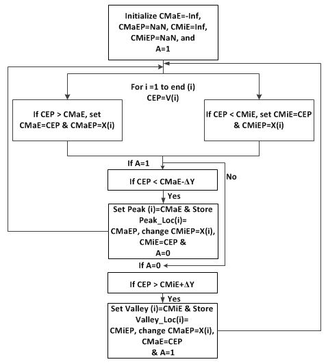
Figure 6 . Flowchart. Peakdet algorithm flow chart.
Step 5: Repeat step 4 until the valleys are detected within the moving window. For a profile, more than one valley could be detected in one wheelpath (i.e., CMiEP and its corresponding CMiE) using the Peakdet algorithm within the 4-m moving window. To be certain the valley detected is not a false positive, the difference between the lowest valley positions (i.e., CMiEPs with minimum CMiEs) for at least two profiles (e.g., the left wheelpath and the center lane) should be less than 0.2 m. The transverse joint locations are common for the three profiles along the entire lane width. However, in the case of skewed joints, the transverse joint location varies for the three profiles and is addressed using a 0.2 m criterion. (It allows detection of the skewed joint, if present.)
One of the CMiEPs from two profiles that meet the 0.2 m criterion is taken as the basis to locate true positive joints for the left and right profiles. Once the true positive joint is detected for a profile, the CEPos of the next moving window would start at 2.5 m (which is 0.625 times the moving window width of 4 m) from the detected joint. The transverse joints on JPCP are spaced at least 3 m from the previous joint except in the case of full-depth patching, which causes joint spacing to be less than 3 m. If the first transverse joint detected for the right profile is at 3.525 m from the start point of the profile section (0 m), then the CEPos of the next moving window would not start from 4.025 to 8 m; rather it would start at 6.025 to 10.025 m, (i.e., 3.525 plus 2.5 m) and would detect the next true positive joint. Thus, potential false positives would be eliminated. In addition, the algorithm checks potential true joint locations with two other profiles taken on the same lane to eliminate spalled joint locations.
Figure 7 and figure 8 illustrate the moving window approach to detect transverse joints using the Peakdet algorithm.
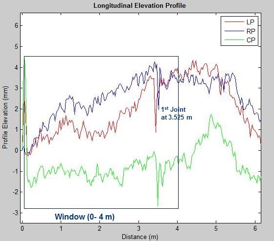
Figure 7 . Graph. A 4-m moving window (0-4 m) using the Peakdet algorithm to detect the first transverse joint.
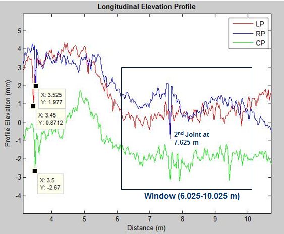
Figure 8 . Graph. A 4-m moving window (6.025-10.025 m) using the Peakdet algorithm to detect the second transverse joint.
Step 6: Repeat step 2 through step 5 to detect all true positive transverse joints, incrementally scanning through the elevation profile and sorting the detected joints. Figure 9 shows the detected transverse joints identified by circles on a longitudinal elevation profile.
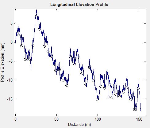
Figure 9 . Graph. Detected true positive transverse joints identified by circles.
The last task is to compute the JPCP transverse joint faulting. Faulting is defined as the difference in elevation across a transverse joint or crack. In this study, faulting is computed using two methods: the slope method (in-house method) and AASHTO R36-12 Method-A. The following steps explain faulting computed using the slope method. For faulting computation using AASHTO R36-12 Method-A, the reader is referred to AASHTO R36-12, "Standard Practice for Estimating Faulting on Concrete Pavements."(3)
The slope method is used to identify the point P1 on the approach slab and point P2 on the leave slab. P1 and P2 are data points on the approach and leave slab. Once P1 and P2 are identified, the faulting can be computed by taking the difference of P1 and P2. If P1 is greater than P2, then the result is called positive faulting. If P1 is less than P2, then the result is called negative faulting. In figure 10, S is absolute slope, and (X1,Y1) and (X2, Y2) are coordinates of points P1 and P2.

Figure 10 . Equation. Two-point slope formula.
To detect P1, the absolute slope is computed using two data points between the detected transverse joint's CMiEP (for example, X2) and CMiE (for example, Y2) and the previous elevation points (for example, X1 and Y1, respectively). If the absolute slope computed is less than 10 (which was selected to make sure the points P1 and P2 are not taken on distressed surface areas such as potholes), then P1 is set equal to Y1. If the absolute slope is not less than 10, then the absolute slope is computed for the closest previous elevation point.
Similarly, to detect P2, the absolute slope is computed using two data points between the detected transverse joint's CMiEP (X2) and CMiE (Y2) and the next location and elevation points (e.g., L1 and E1). If the absolute slope computed is less than 10, then P2 is set equal to E1. If the absolute slope is not less than 10, then the absolute slope is computed for the next elevation point.
Once the joint faulting is computed, the results are exported in Microsoft® Excel format.
Figure 11 illustrates the slope method to compute transverse joint faulting. The traverse joint location is first located, and then points P1 on the approach slab and P2 on the leave slab are established. The transverse joint location was detected at distance 3.525 m (X) and elevation 1.977 mm (Y). The computed absolute slope between the detected transverse joint coordinates (X at 3.525 m and Y at 1.977 mm) and the previous profile data point (X at 3.5 m and Y at 2.759 mm) was more than 10, so the procedure was continued until P1 was reached at X equal to 3.475 m and Y equal to 4.165 mm. Similarly, the computed absolute slope between the detected transverse joint location (X at 3.525 m and Y at 1.977 mm) and the next profile data point (X at 3.55 m and Y at 3.992 mm) was more than 10, so the procedure was continued until P2 was reached at X equal to 3.575 m and Y equal to 3.794 mm. Thus, the elevation (Y) of P1 on the approach slab was 4.165 mm, and the elevation of P2 on the leave slab was 3.794 mm. The faulting computed at the joint location was therefore 0.371 mm (4.165 minus 3.794). This slope method approach was used to compute faulting at all detected transverse joint locations.
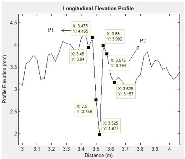
Figure 11 . Graph. The slope method to determine P1 on approach slab and P2 on leave slab.