U.S. Department of Transportation
Federal Highway Administration
1200 New Jersey Avenue, SE
Washington, DC 20590
202-366-4000
Federal Highway Administration Research and Technology
Coordinating, Developing, and Delivering Highway Transportation Innovations
 |
| This report is an archived publication and may contain dated technical, contact, and link information |
|
Publication Number: FHWA-RD-02-001 |
Accurate and reliable information about pavement material properties is key to predicting the states of stress, strain, and displacement within the pavement structure when subjected to an external wheel and climate-related loading. Computed stress and strain are then used as critical responses that are needed for predicting distress and pavement performance. For example, Portland cement concrete (PCC) cracking is related to the PCC flexural strength, and pumping and faulting can be related to the erodibility of the underlying base/subbase material. The inclusion of accurate material-related data is, therefore, vital in research studies such as the Long-Term Pavement Performance (LTPP) study.
This report documents the state of selected material-related data elements in the LTPP material characterization program. The data were evaluated to assess completeness and quality. Recommendations are also provided regarding the suitability of the data evaluated for future research and analysis. The report also provides information on representative data tables developed as part of this study and recommended for inclusion in the LTPP database. The report is intended for all LTPP data users--from those with considerable experience to those with no familiarity with the LTPP database.
T. Paul Teng, P.E.
Director
Office of Infrastructure
Research and Development
This document is distributed under the sponsorship of the Department of Transportation in the interest of information exchange. The U.S. Government assumes no liability for its contents or use thereof. This report does not constitute a standard, specification, or regulation.
The U.S. Government does not endorse products or manufacturers. Trade and manufacturers' names appear in this report only because they are considered essential to the object of the document.
1. Report No.: FHWA-RD-02-001
2. Government Accession No.:
3. Recipient's Catalog No.:
4. Title and Subtitle: ASSESSMENT OF SELECTED LTPP MATERIAL DATA TABLES AND DEVELOPMENT OF REPRESENTATIVE TEST TABLES
5. Report Date:
6. Performing Organization Code:
7. Author(s): Leslie Titus-Glover, Jagannath Mallela, Y. Jane Jiang, Michael E. Ayers, and Haroon I. Shami
8. Performing Organization Report No.:
9. Performing Organization Name and Address: ERES Consultants, 9030 Red Branch Road, Suit 210, Columbia, MD 21045
10. Work Unit No. (TRAIS): C6B
11. Contract or Grant No.: DTFH61-96-C-00003
12. Sponsoring Agency Name and Address: Office on Infrastructure Research and Development, Federal Highway Administration, 6300 Georgetown PikeMcLean, Virginia 22101-2296
13. Type of Report and Period Covered: Final Report, September 1999 to August 2001
14. Sponsoring Agency Code:
15. Supplementary Notes: Contracting Officer's Technical Representative (COTR): Cheryl Allen Richter, P.E., HRDI-13
16. Abstract:
This report documents an evaluation of selected LTPP material data tables as of January 2000. Issues addressed include the availability, characteristics, and quality of the data in the selected tables. Anomalies in the data were identified and corrected where possible, and the "cleaned-out" data were used in developing representative data tables. Recommendations for adjustments in the current data collection process are also presented.
17. Key Words: Bias, concrete pavement, paving materials, precision, variability.
18. Distribution Statement: No restrictions. This document is available to the public through the National Technical Information Service, Springfield, VA 22161.
19. Security Classification (of this report): Unclassified
20. Security Classification (of this page): Unclassified
21. No. of Pages: 304
22. Price:
Form DOT F 1700.7 (8-72)
Reproduction of completed page authorized
Approximate Conversions to SI Units
Length:
inches (in) multiply by 25.4 to get millimeters (mm)
feet (ft) multiply by 0.305 to get meters (m)
yards (yd) multiply by 0.914 to get meters (m)
miles (mi) multiply by 1.61 to get kilometers (km)
Area:
square inches (in2) multiply by 645.2 to get square millimeters (mm2)
square feet (ft2) multiply by 0.093 to get square meters (m2)
square yard (yd2) multiply by 0.836 to get square meters (m2)
acres (ac) multiply by 0.405 to get hectares (ha)
square miles (mi2) multiply by 2.59 to get square kilometers (km2)
Volume:
fluid ounces (fl oz) multiply by 29.57 to get milliliters (mL)
gallons (gal) multiply by 3.785 to get liters (L)
cubic feet (ft3) multiply by 0.028 to get cubic meters (m3)
cubic yards (yd3) multiply by 0.765 to get cubic meters (m3)
NOTE: volumes greater than 1000 L shall be shown in m3
Mass:
ounces (oz) multiply by 28.35 to get grams (g)
pounds (lb) multiply by 0.454 to get kilograms (kg)
short tons - 2000 lb (T) multiply by 0.907 to get megagrams or "metric ton" (Mg or "t")
Temperature (exact degrees):
Fahrenheit (°F) multiply by 5 (F-32)/9 or (F-32)/1.8 to get Celsius (°C)
Illumination:
foot-candles (fc) multiply by 10.76 to get lux (lx)
foot-Lamberts (fl) multiply by 3.426 to get candela/m2 (cd/m2)
Force and Pressure or Stress:
poundforce (lbf) multiply by 4.45 to get newtons (N)
poundforce per square inch (lbf/in2) multiply by 6.89 to get kilopascals (kPa)
Approximate Conversions From SI Units
Length:
millimeters (mm) multiply by 0.039 to get inches (in)
meters (m) multiply by 3.28 to get feet (ft)
meters (m) multiply by 1.09 to get yards (yd)
kilometers (km) multiply by 0.621 to get miles (mi)
Area:
square millimeters (mm2) multiply by 0.0016 to get square inches (in2)
square meters (m2) multiply by 10.764 to get square feet (ft2)
square meters (m2) multiply by 1.195 to get square yards (yd2)
hectares (ha) multiply by 2.47 to get acres (ac)
square kilometers (km2) multiply by 0.386 to get square miles (mi2)
Volume:
milliliters (mL) multiply by 0.034 to get fluid ounces (fl oz)
liters (L) multiply by 0.264 to get gallons (gal)
cubic meters (m3) multiply by 35.314 to get cubic feet (ft3)
cubic meters (m3) multiply by 1.307 to get cubic yards (yd3)
Mass:
grams (g) multiply by 0.035 to get ounces (oz)
kilograms (kg) multiply by 2.202 to get pounds (lb)
megagrams or "metric ton" (Mg or "t") multiply by 1.103 to get short tons - 2000 lb (T)
Temperature (exact degrees):
Celsius (°C) multiply by 1.8C+32 to get Fahrenheit (°F)
Illumination:
lux (lx) multiply by 0.0929 to get foot-candles (fc)
candela/m2 (cd/m2) multiply by 0.2919 to get foot-Lamberts (fl)
Force and Pressure or Stress:
newtons (N) multiply by 0.225 to get poundforce (lbf)
kilopascals (kPa) multiply by 0.145 to get poundforce per square inch (lbf/in2)
*SI is the symbol for the International System of Units. Appropriate rounding should be made to comply with Section 4 of ASTM E380.
(Revised March 2002)
Overview of LTPP Material Characterization Program
Objectives of the Materials Assessment Study
Scope of the Report
2. OVERVIEW OF LTPP MATERIALS CHARACTERIZATION PROGRAM
Introduction
Material Data Collection Process
Material Sampling
Material Handling
Laboratory Testing
Data Processing
Material Data Elements Evaluated for the Current Study
3. OVERVIEW OF DATA QUALITY EVALUATION TECHNIQUES AND PROCEDURES FOR COMPUTING NEW DATA ELEMENTS
Assembly and Preparation of Selected Data Elements
Assessing Data Completeness
Assessing Data Quality
Recommendations for Remedial Action to Correct Identified Anomalies
4. AC CORE EXAMINATION AND THICKNESS
Introduction
Material Sampling for AC Core Thickness
AC Core Data Completeness
AC Core Visual Examination and Thickness Data Quality
Identification of Anomalous Data
Schema of the Representative AC Core Examination and Thickness Data Table (TST_AC01_LAYER_REP)
5. BULK SPECIFIC GRAVITY OF AC CORES
Introduction
Material Sampling for Bulk Specific Gravity of AC Cores
Bulk Specific Gravity Data Completeness
Bulk Specific Gravity of AC Cores Data Quality
Identification of Anomalous Data
Schema of the Representative Bulk Specific Gravity of AC Cores Tables (TST_AC02_REP_GPS and TST_AC02_REP_SPS)
6. MAXIMUM SPECIFIC GRAVITY OF ASPHALT CONCRETE
Introduction
Material Sampling for AC Maximum Specific Gravity Testing
Data Completeness for Maximum Specific Gravity of AC Cores
MSG Data Quality
Identification of Anomalous Data
Schema of the Revised MSG Data Table TST_AC03_REP
7. ASPHALTIC CONTENT OF ASPHALTIC CONCRETE
Introduction
Material Sampling for Asphalt Content of AC Mixtures
Data Completeness for Asphalt Content of AC Mixtures
Asphalt Content Data Quality Evaluation
Identification of Anomalous Data
Schema of the Representative Asphalt Content of AC Data Tables (TST_AC04_REP_GPS and TST_AC04_REP_SPS)
8. MOISTURE SUSCEPTIBILITY OF ASPHALT CONCRETE
Introduction
Overview of Moisture Susceptibility Test Methods
Material Sampling for AC Moisture Susceptibility Testing
Data Completeness for Moisture Susceptibility Data Quality Assessment of Moisture Susceptibility of Asphalt Concrete Data
Identification of Anomalous Data
Schema of the Representative Moisture Susceptibility Data Table TST_AC05_REP
Recommendations
9. VISUAL EXAMINATION AND LENGTH MEASUREMENT OF PCC CORES
Introduction
Material Sampling
PCC Core Thickness Data Completeness
Thickness and Visual Examination Data Quality
Identification of Anomalous Data
Schema for Table TST_PC06_REP-Representative Length Measurements for PCC and LCB Cores
10. DETERMINATION OF COMPRESSIVE STRENGTH OF PORTLAND CEMENT CONCRETE CORES
Introduction
Material Sampling for Compressive Strength Testing
Compressive Strength Data Completeness
Compressive Strength Data Quality
Identification of Anomalous Data
Schema for Representative PCC Compressive Strength Data Table (TST_PC01_REP)
11. DETERMINATION OF THE COEFFICIENT OF THERMAL EXPANSION OF PORTLAND CEMENT CONCRETE
Introduction
Material Sampling for the Determination of CTE
CTE Data Completeness
CTE Data Quality
Identification of Anomalies
Schema for the Representative PCC CTE Data Table (TST_PC03_REP)
12. FLEXURAL STRENGTH OF PORTLAND CEMENT CONCRETE
Introduction
Material Sampling for Flexural Strength Testing
Flexural Strength Data Completeness
Flexural Strength Data Quality
Summary of Flexural Strength Data Evaluation
Identification of Anomalous Data
Schema for the Representative PCC Flexural Strength Data Table (TST_PC09_REP)
13. COMPRESSIVE STRENGTH OF OTHER THAN ASPHALT TREATED BASE AND SUBBASE MATERIALS
Introduction
Material Sampling for OTB Compressive Strength Determination
Experiment Type
OTB Compressive Strength Data Completeness
OTB Compressive Strength Data Quality
Identification of Anomalous Data
Schema for the Representative OTB Compressive Strength Data Table (TST_TB02_REP)
14. ATTERBERG LIMITS OF SUBGRADE SOILS
Introduction
Material Sampling for Determining Atterberg Limits of Subgrade Soils
Data Completeness for Atterberg Limits of Subgrade Soils
Atterberg Limits of Subgrade Soils Data Quality Assessment
Atterberg Limits Data Quality
Identification of Anomalous Data
Schema for the Representative Atterberg Limits Data Tables (TST_UG04_SS03_REP_GPS and TST_ UG04_SS03_REP_SPS)
15. UNCONFINED COMPRESSIVE STRENGTH OF SUBGRADE SOILS
Introduction
Material Sampling for Unconfined Compressive Strength Testing of Subgrade Soils
Data Completeness for Unconfined Compressive Strength
Quality Assessment of Unconfined Compressive Strength of Subgrade Soils
Assessing Unconfined Compressive Strength Data Quality
Identification of Anomalous Data
Schema for the Representative Unconfined Compressive Strength Data Table (TST_SS10_REP)
16. PARTICLE SIZE ANALYSIS OF UNBOUND BASE, SUBBASE, EMBANKMENT, AND SUBGRADE MATERIALS
Introduction
Material Sampling for Particle Size Analysis
Gradation Data Completeness
Gradation of Unbound Base, Subbase, and Subgrade Test Data Quality
Identification of Anomalous Data
Schema for the Representative Particle Size Analysis of Unbound Base, Subbase, Embankment, and Subgrade Materials Data Table (TST_ SS01_UG01_UG02_REP)
17. GRADATION OF AGGREGATE EXTRACTED FROM ASPHALTIC CONCRETE
Introduction
Material Sampling
Gradation Data Completeness
Gradation of Extracted Aggregate from Asphaltic Concrete Data Quality
Identification of Anomalous Data
Schema for the Representative Gradation of Aggregate Extracted from Asphaltic Concrete Data Table (TST_ AG04_REP)
18. CONCLUSIONS AND RECOMMENDATIONS
Conclusions
Recommendations
Summary
1. Material data elements evaluated
2. Descriptive statistics for evaluating reasonableness of test data
3. Potential anomalies in material test data and recommended remedial action
4. Sampling requirements for visual examination and thickness of AC cores
6. Data fields used for defining analysis cells for AC thickness
7. Level 1 data completeness for table TST_AC01_LAYER
8. Summary of level 2 data completeness for TST_AC01_LAYER
9. Range of thickness for various GPS AC layers
10. Summaries of descriptive statistics for core thickness data in table TST_AC01_LAYER
11. Typical variability for HMAC- and asphalt-treated layers
12. Data fields used for defining analysis cells for BSG
13. Sampling and testing requirements for BSG of AC cores for GPS experiments
14. Details of sampling and testing requirements for BSG of AC cores for SPS experiments
15. Level 1 data completeness for table TST_AC02
16. Summary of level 2 data completeness for table TST_AC02
17. Typical values of specific gravity for selected aggregate
18. Summary of nontypical BSG test data
19. Typical variability for air voids
20. Schema for representative data tables TST_AC02_REP_GPS and TST_AC02_REP_SPS
21. Data fields used for defining analysis cells for BSG
22. Sampling and testing requirements for MSG of AC for GPS experiments
23. Details of sampling and testing requirements for MSG for SPS experiments
24. Level 1 data completeness for AC03 table
25. Level 2 data completeness assessment for table TST_AC03
26. MSG testing recommended variability
27. Schema for representative data tables TST_AC02_REP_GPS and TST_AC02_REP_SPS
28. Sampling and testing requirements for extracted asphalt content
29. Sampling and testing requirements for extracted asphalt content for SPS projects
30. Data fields used for defining analysis cells for asphalt content
31. Summary of level 1 data completeness evaluation for asphalt content
32. Level 2 data completeness from asphalt content data
33. Summary of typical variability in asphalt content field data.(13)
34. Schema for tables TST_AC04_REP_GPS and TST_AC04_REP_SPS
35. Sampling and testing requirements for moisture susceptibility of bituminous mixtures
36. Data fields used for defining analysis cells for AC moisture susceptibility
37. Level 1 completeness for table TST_AC05
38. Summary of level 2 data completeness assessment for table TST_AC05
39. Summary of average core thickness data available in table TST_PC06
40. Analysis cell definitions for test table TST_PC06
42. Details of sampling for core visual examination and length measurement for SPS experiments
43. Summary of core thickness data available for GPS and SPS experiments
44. Summaries of descriptive statistic for core thickness data in table TST_PC06
45. Typical allowable variability for thickness data
46. Description of visual survey codes
47. Sampling requirements for determination of compressive strength of PCC materials
48. Summary of compressive strength data in table TST_PC01 in the LTPP database
49. Analysis cell definitions for test table TST_PC01
50. Summary of level 2 data completeness analysis of data from TST_PC01 for GPS experiment sections
51. Summary of SPS-2 level 2 data completeness analysis for LCB layers
52. Summary of SPS-2 level 2 data completeness analysis for PCC layers
53. Summary of SPS-6 level 2 data completeness analysis
54. Summary of SPS-7 level 2 data completeness analysis
55. Summary of SPS-8 level 2 data completeness analysis
56. Typical variability for 28-day compressive strength data
57. Variation of concrete compressive strength with age and curing conditions
58. Sampling for determination of CTE of PCC
59. Summary of PCC CTE data available in test table TST_PC03
60. Summary of flexural strength data available in LTPP database table TST_PC09
61. Sampling for determination of in-place concrete flexural strength
62. Summary of flexural strength data available for SPS experiments
63. Typical allowable variability for flexural strength
64. Normalized 14-, 28-, and 365-day flexural strengths estimated using equation 11
65. Models for relating compressive to flexural strength
66. Sampling requirements for the determination of compressive strength of OTB materials
67. Summary of level 1 data completeness analysis for TST_TB02
68. Analysis cell definitions for test table TST_TB02
69. Summary of level 2 data completeness analysis for TST_TB02
70. Sampling and testing requirements for Atterberg limits of subgrade soils
71. Fields used in defining analysis cells for table TST_ UG04_SS03 data evaluation
72. Level 1 data completeness for table TST_UG04_SS03
73. Summary of level 2 data completeness evaluation for table TST_UG04_SS03
74. Liquid and plastic limits of various soils
75. Recommended variability for liquid and plastic limit test results
76. Summary of typical variability within liquid and plastic limit test results
78. Sampling and testing requirements for unconfined compressive strength of subgrade soils
79. Fields used in defining analysis cells for table TST_ UG04_SS03 data evaluation
80. Level 1 completeness for table TST_SS10
81. Level 2 data completeness evaluation for table TST_SS10
83. Typical variability for unconfined compressive strength testing
85. Summary of level 1 data completeness for TST_ SS01_UG01_UG02
87. Summary of level 2 data completeness for TST_SS01_UG01_UG02
88. Summary of particle size analysis data available for SPS experiments
89. Percentage of analysis cells with potentially biased results due to inadequate sampling
90. Summary of recommended test sample weight for gradation testing
91. Precision for coarse aggregate fraction
92. Precision for fine aggregate particle size analysis
93. Typical allowable variability for gradation of unbound materials
94. Summary of test data quality for LTPP table TST_SS01_UG01_UG_02
95. Summary of particle size analysis data available in LTPP database
96. Sampling and testing requirements for gradation of extracted aggregates
97. Summary of gradation data available for GPS sections
98. Summary of gradation data available for SPS experiments
99. Percentage of analysis cells with potentially biased results due to inadequate sampling
100. Precision for coarse aggregate fraction
101. Typical allowable variability for gradation of extracted aggregates from asphaltic concrete
102. Summary of test data quality for LTPP table TST_AG04
103. Summary of existing and new tables developed
104. Summary of data completeness analyses for all the data elements considered
105. Test table categories based on data completeness analysis
1. Layout of GPS and SPS experiments
2. Summary of data tables evaluation procedure
3. Example of typical analysis cells for a GPS test pavement
4. Flow chart for assessing data quality
5. Scatter diagram used in assessing reasonableness of data
6. Time-series plot used in data quality evaluation
8. Summation of testing, sampling, and material variability to yield typical variability
9. Relationship between precision, accuracy, and bias
10. Distribution of AC core thickness for base layers
11. Distribution of AC core thickness for surface layers
12. Distribution of AC core thickness for overlays
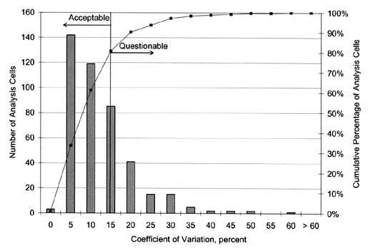
13. Distribution of COV for analysis cells from GPS experiments
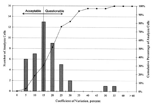
14. Distribution of COV for analysis cells from SPS experiments
15. Distribution of BSG test results for GPS surface layers
16. Distribution of BSG test results for GPS base layers
17. Frequency distribution of BSG measurements for all dense-graded HMAC of SPS surface layers
18. Frequency distribution of BSG measurements for all dense-graded HMAC of SPS base layers
19. Distribution of COV of BSG for GPS analysis cells
20. Distribution of COV of BSG for SPS analysis cells
21. Distribution of MSG test results for GPS experiments (surface layers)
22. Distribution of MSG test results for GPS experiments (base layers)
23. Distribution of MSG test results for GPS experiments (surface layers)
24. Distribution of MSG test results for SPS experiments (base layers)
25. Distribution of COV for MSG analysis cells from GPS experiments
26. Distribution of COV for MSG analysis cells from SPS experiments
27. Distribution of asphalt content for HMAC surface material for GPS experiments
28. Distribution of asphalt content for HMAC surface material for SPS experiments
29. Distribution of asphalt content measurements for HMAC base layers from GPS experiments
30. Distribution of asphalt content measurements for HMAC base layers from SPS experiments
31. Distribution of COV of asphalt content analysis cells from GPS experiments
32. Distribution of COV of asphalt content analysis cells from SPS experiments
33. Distribution of the TSR in table TST_AC05
34. Distribution of COV for TSR
35. Histogram of PCC core specimen data availability for GPS pavement sections
36. Histogram of PCC core specimen data availability for SPS pavement sections
37. Plots of distribution of core thickness for SPS-7 75-mm overlay sections
38. Plots of distribution of core thickness for SPS-7 125-mm overlay sections
39. Distribution of standard deviation for pavement test sections thickness with complete testing
40. Distribution of standard deviation for pavement section thickness with incomplete testing
41. Summary of visual examination comments for all core specimens
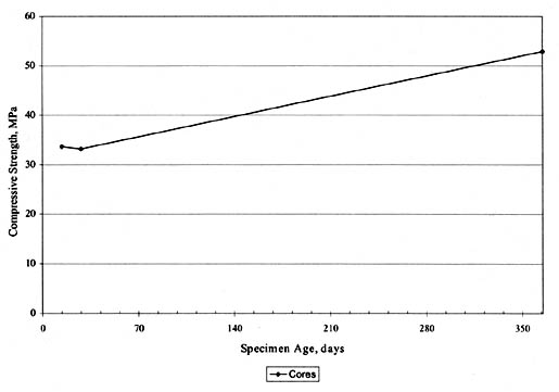
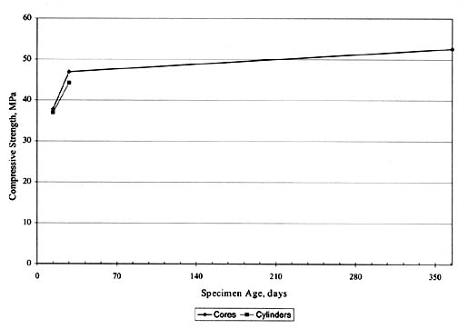
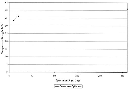
42. Long-term compressive strength data from GPS, SPS-6, and SPS-7
43. Time-series plots of SPS-2 LCB compressive strength data for State 4
44. Time-series plots of SPS-2 LCB compressive strength data for State 10
45. Time-series plots of SPS-2 LCB compressive strength data for State 19
46. Time-series plots of SPS-2 LCB compressive strength data for State 20
47. Time-series plots of SPS-2 LCB compressive strength data for State 26
48. Time-series plots of SPS-2 LCB compressive strength data for State 32
49. Time-series plots of SPS-2 LCB compressive strength data for State 39
50. Time-series plots of SPS-2 LCB compressive strength data for State 53
51. Time-series plots of SPS-2 PCC compressive strength data for State 4
52. Time-series plots of SPS-2 PCC compressive strength data for State 8
53. Time-series plots of SPS-2 PCC compressive strength data for State 10
54. Time-series plots of SPS-2 PCC compressive strength data for State 19
55. Time-series plots of SPS-2 PCC compressive strength data for State 20
56. Time-series plots of SPS-2 PCC compressive strength data for State 26
57. Time-series plots of SPS-2 PCC compressive strength data for State 32
58. Time-series plots of SPS-2 PCC compressive strength data for State 37
59. Time-series plots of SPS-2 PCC compressive strength data for State 38
60. Time-series plots of SPS-2 PCC compressive strength data for State 39
61. Time-series plots of SPS-2 PCC compressive strength data for State 53
62. Time-series plots of SPS-7 PCC compressive strength data for State 19
63. Time-series plots of SPS-7 PCC compressive strength data for State 22
64. Time-series plots of SPS-7 PCC compressive strength data for State 29
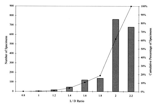
65. L/D ratio representation in table TST_PC01 (all experiments)
66. Intersample variability of PCC compressive strength data (all experiments)
67. Intersample variability of LCB compressive strength data (SPS-2)
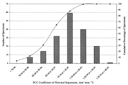
68. Scatter plot of CTE data for all PCC sections in table TST_PC03
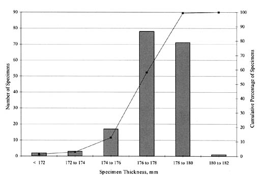
69. Sample thickness variability for all records in TST_PC03
70. Histogram of flexural strength data availability for SPS pavement sections
71. Time-series plot of modulus of rupture versus specimen age for SPS-2 experiments in State 10
72. Time-series plot of modulus of rupture versus specimen age for SPS-2 experiments in State 19
73. Time-series plot of modulus of rupture versus specimen age for SPS-2 experiments in State 20
74. Time-series plot of modulus of rupture versus specimen age for SPS-2 experiments in State 32
75. Time-series plot of modulus of rupture versus specimen age for SPS-2 experiments in State 39
76. Time-series plot of modulus of rupture versus specimen age for SPS-2 experiments in State 53
77. Time-series plot of modulus of rupture versus specimen age for SPS-7 experiment in State 22
78. Distribution of within-cell COV for PCC flexural strength data
79. Diagram of the flexural test of concrete using the third-point loading method (ASTM C78)
80. Stress distribution across the depth of a concrete specimen in flexure
81. Plot showing the relationship between strength ratio and specimen age in days
82. Scatter plot of compressive strength data for all cement aggregate specimens in TST_TB02
83. Scatter plot of compressive strength data for all lean concrete specimens in TST_TB02
84. Sample thickness variability for all records in TST_TB02
85. Sample L/D ratio variability for all records in TST_TB02
86. Intersample variability for cement aggregate and LCB compressive strength data
87. Influence of the L/D ratio on the apparent strength of a cylinder for different strength levels
88. Distribution of liquid limit measurements for fine-grained soils (GPS experiments)
89. Distribution of liquid limit measurements for coarse-grained soils (GPS experiments)
90. Distribution of liquid limit measurements for fine-grained soils (SPS experiments)
91. Distribution of liquid limit measurements for coarse-grained soils (SPS experiments)
92. Distribution of plastic limit measurements for fine-grained soils (GPS experiments)
93. Distribution of plastic limit measurements for coarse-grained soils (GPS experiments)
94. Distribution of plastic limit measurements for fine-grained soils (SPS experiments)
95. Distribution of plastic limit measurements for coarse-grained soils (SPS experiments)
96. Distribution of COV for liquid limit analysis cell from GPS experiments
97. Distribution of COV for liquid limit analysis cell from SPS experiments
98. Distribution of COV for plastic limit analysis cell from GPS experiments
99. Distribution of COV for plastic limit analysis cell from SPS experiments
100. Distribution of unconfined compressive strength values for fine-grained subgrade soils
101. Distribution of unconfined compressive strength values for coarse-grained subgrade soils
102. Distribution of COV for analysis cells in table TST_SS10
103. Histogram showing gradation data availability for GPS experiments
104. Histogram showing gradation data availability for SPS experiments
105. Example of plots used in assessing the gradation data reasonableness
108. Histogram showing gradation data availability for GPS experiments
109. Histogram showing gradation data availability for SPS experiments
110. Examples of plots used in assessing the gradation data reasonableness
111. Summary of data completeness analysis
Information about pavement material properties is required to predict states of stress, strain, and displacement within the pavement structure when subjected to an external wheel load. In both empirical and mechanistic-empirical (M-E) design systems, material properties such as elastic modulus (E), compressive strength (fc), Poisson's ratio (mu), tensile strength (ft), and flexural strength (MR) are mandatory inputs for characterizing pavement systems, computing pavement critical responses (e.g., stress and strain) to applied traffic and climate-related loads, and predicting performance.
Material characterization is vital to pavement design because most of the major distresses that occur in pavements can be associated with the material properties of a component or layer of the pavement structure. For example, portland cement concrete (PCC) cracking is related to the PCC flexural strength, and pumping and faulting can be related to the erodibility of the underlying base/subbase material. Material characterization is also vital in research studies, such as the Federal Highway Administration (FHWA) Long-Term Pavement Performance (LTPP) study, to determine the effects of material properties on pavement performance.
This report documents the state of selected material-related data elements in the LTPP material characterization program. The data were evaluated to assess completeness and quality. Recommendations are also provided regarding the suitability of the data evaluated for future research and analysis.
Overview of LTPP Material Characterization Program
One of the important objectives of the LTPP program is to understand the relationship between pavement material properties and pavement performance. A better understanding of this relationship will ensure that appropriate materials are specified and used in pavement construction to provide the desired level of performance. LTPP material characterization, therefore, serves the following purposes:(1)
Material Characterization
The LTPP material characterization program was implemented by:(1)
As of January 2000, over 775 GPS and SPS sites have been sampled as part of the material characterization program. Sampling from these sites included the extraction of almost 14,000 cores (200 tons of bulk samples), the excavation of over 450 test pits, and the performance of over 330 in situ nuclear density tests.(1)
The sampling and testing program was conducted on the following materials:
An overview of each category is presented in the following sections.
Asphalt Binder/Cement
Asphalt cement is obtained by the distillation of crude petroleum. At ambient temperatures, it is a black, sticky, semisolid, highly viscous material. The primary use of asphalt cement is to produce AC and asphalt-treated materials for use in the construction of flexible pavements.
The properties of the asphalt cement used in producing AC have a significant influence on the final AC properties. Some of the important AC properties influenced by asphalt cement are:
Several tests are performed on new and extracted asphalt cement materials as part of the LTPP materials characterization program.
Asphalt Concrete
Asphalt concrete describes a broad range of aggregate and filler materials bound together with asphalt cement. It is normally used as the wearing, binder, base, and/or subbase layers of a flexible pavement. Their properties and behavior are heavily influenced by temperature, time rate of loading, mixture proportions, and construction. This category of pavement materials includes many different subgroups--ranging from the hot mix asphalt layer to the asphalt-treated sand. Thus, there is a great deal of variability in properties, behavior, and suitability for pavement design and construction.
Portland Cement and Portland Cement Concrete
Portland cement is the principal strength-giving and property-controlling component of PCC. It is a hydraulic cement that gains strength as it reacts with water. Although the reaction is initially fairly rapid (approximately 40 percent occurs within the first 24 hours), it slows down considerably with the passage of time. The hydration reaction produces a finely divided, fairly porous solid between the fine and coarse aggregate particles in PCC. Portland cement properties are, thus, very important for PCC material design and research into PCC strength and durability.
Cement-Treated Materials/Cementitious Materials
Cement-treated/cementitious materials include lean concrete, lime, and other pozzolanic (chemical)-treated soils. Their properties range from materials that only slightly modify the plasticity characteristics of the original aggregate/soil material to materials having major gains in stiffness, strength, and other key engineering properties. Lime, flyash, and cement are the major types of cementing material in this category.
Unbound Base/Subbase
The major material characteristics associated with unbound base/subbase materials are related to the fact that the strength and deformation of these materials are highly influenced by the stress state (nonlinear) and in situ moisture content. As a general rule, coarse-grained materials become more stiff as the state of stress is increased. In contrast, clay materials tend to have a reduction in stiffness as the deviatoric or octahedral stress component is increased. Thus, although both categories of unbound materials are stress dependent (nonlinear), each behaves in an opposite direction as stress states are increased.
Subgrade
The subgrade provides the foundation of a pavement system. Subgrade characterization is, therefore, an important component of pavement design and construction. Subgrade properties such as gradation, plasticity, strength, moisture sensitivity, permeability, and frost susceptibility are important for characterizing pavement subgrade materials for pavement design.
Characterizing subgrade material variability is key for assessing the reliability of pavement designs. This is especially true for pavements constructed directly over natural subgrade with no form of modifications or treatment with lime, asphalt, or cement.
Laboratory Testing
The LTPP laboratory testing process, conducted to establish material properties and characteristics, involved more than 40 test procedures, including thickness determinations, compressive strength, gradation, Atterberg limits, and resilient modulus.(1)
The sampling and laboratory testing were conducted using Strategic Highway Research Program (SHRP) test protocols documented in the SHRP Laboratory Material Handling and Testing Guide.(2) Most of the testing protocols were based on the American Society for Testing and Materials (ASTM) and American Association of State Highway and Transportation Officials (AASHTO) approved procedures.(3, 4) Data obtained through material characterization tests are stored in the Materials module in the LTPP database, which currently consists of 76 separate tables containing various data elements obtained through testing.(5)
Objectives of the Materials Assessment Study
This study has the following objectives:
Efforts to achieve these objectives were divided into two phases. The scope of Phase I was as follows:
Phase II of the study consisted of tasks to resolve anomalies identified in Phase I to reduce excessive variability in the data and to compute representative test values and new parameters. The scope of Phase II was as follows:
Scope of the Report
This report presents the work done to improve the LTPP material data quality and to include new data elements in the database. It addresses work done in assessing and evaluating material data availability and quality of the available data. Chapter 2 of this report presents an overview of the LTPP material characterization program, with emphasis placed on the key material-related data elements being evaluated as part of this study. Chapter 3 discusses various methodologies for assessing data availability, data quality, performance of remedial action, and computing of representative test values.
Chapters 4 through 17 present a detailed summary of data availability and quality for the 13 data elements evaluated in this study. They also present detailed documentation of the procedures used in correcting anomalies, computing missing test results, and computing representative test values and other basic statistics.
Chapter 18 presents conclusions and recommendations. Issues discussed in chapter 18 include the adequacy of current LTPP material data-collection procedures, the need for computing new data elements with respect to meeting future analysis needs, and recommendations for collecting (through sampling and testing) material-related data elements that are not currently available but may be needed for future analysis efforts.
Introduction
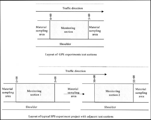
The LTPP program consists of two complementary experiments, GPS and SPS. GPS experiments are usually existing in-service pavements incorporated into the LTPP program, whereas the SPS experiments are newly constructed or rehabilitated pavements or pavements subjected to various forms of maintenance activities. GPS experiments consist of a single 152-m pavement test section, whereas SPS experiments usually consist of a series of adjacent 152-m test sections with different design and material characteristics or maintenance treatments and rehabilitation strategies. The various GPS and SPS experiments are as follows:(1)
Figure 1 shows the typical layout of GPS and adjacent SPS test sections (projects) within an experiment. The typical SPS experiment consists of 12 test sections at a project site.
Material Data Collection Process
Material characterization, distress, climate, traffic, inventory, and other types of data are collected and stored in the LTPP database by four LTPP regional offices, supervised by the LTPP staff. Each regional office is responsible for data collection in a specific group of States, Provinces, and Territories.(1) For material characterization, the regional offices focus on:
The technical support contractor is responsible for quality assurance (QA) of all LTPP data. It is also responsible for providing the data to the public and assists the LTPP staff in ensuring that common test procedures and standards are used, so that there is consistency in the data-collection process and quality control (QC) is maintained at all times in the material characterization program. Specific procedures employed to maintain QC are discussed in the next section.
Material Sampling
The LTPP materials characterization effort begins with field sampling and laboratory testing of the sampled paving materials. Undisturbed material samples or disturbed bulk samples are obtained by drilling, coring, or excavating test pits at designated locations within the pavement test sections. Sampling was performed using the plans and guidelines provided in the Laboratory Material Handling and Testing Operational Guide.(2)
For GPS experiments, samples were marked and shipped to the designated laboratories for testing by the LTPP regional field material sampling and field testing contractors. For SPS experiments, the samples were marked and shipped to the designated laboratories for testing by the local highway agencies or tested in the agency laboratory facilities. Conditions encountered in the field while sampling were recorded and documented to provide the laboratories with adequate background information on the materials to be tested.
The typical LTPP pavement test section consists of an area 152-m long and one lane wide. Nondestructive tests, such as Falling Weight Deflectometer (FWD) tests to obtain pavement deflection under loading and visual surveys to obtain distress data such as cracks and ruts, are conducted periodically on these sections to characterize pavement performance.1 For this reason, paving materials for laboratory characterization were retrieved only from the beginning and the end of the designated test sections (just outside the 152-m limits). Sufficient space is left between the adjacent test sections in SPS experiments to facilitate the drilling and retrieval of paving materials for testing. Details of sampling location and dimensions of cores or test pits for the different LTPP experiments are provided in the Laboratory Material Handling and Testing Operational Guide.(2)
1 For a complete history of and information regarding the frequency of NDT and visual distress surveys, refer to appropriate FHWA reference manuals and reports.
Material Handling
After retrieving sample materials from coring or test pits, the sample materials were marked and labeled for easy identification before shipping to the testing laboratory. As a minimum, the following information was included on tags and labels:
Laboratory tests were performed on several paving materials, including AC, extracted aggregate from the AC, treated base and subbase, untreated base and subbase, subgrade, and PCC materials. The tests were performed according to test protocols found in the SHRP Interim Guide for Laboratory Material Handling and Testing.(2)
Laboratory Testing
Laboratory testing includes both the material preparation and the actual testing of samples. Testing is done only by accredited laboratories. Accredited laboratories are expected to provide sufficient and suitable materials testing equipment, facilities, and personnel to meet the requirements of ASTM E329-77, ASTM D3666-83, ASTM D3740-80, and the AASHTO Accreditation Program (AAP), as outlined in the AASHTO Technical Provisions.(3, 4)
Material sampling and testing is performed at least once at the beginning of the section's acceptance into the LTPP program. Additional testing may be performed because of the study requirements or to investigate unexpectedly poor performance. Materials test data are stored in the Materials module in the LTPP database.
Data Processing
LTPP material data processing begins with sample retrieval in the field and continues throughout material characterization until the test results and associated data are placed in the LTPP database at the highest data quality level. Several QA/QC checks are built into the data processing mechanism to ensure that the final data are of the highest quality. Step-by-step operational procedures to ensure QA/QC can be found in several SHRP publications, including LTPP IMS Data Quality Checks and the SHRP Interim Guide for Laboratory Material Handling and Testing.(2, 6) The following basic definitions related to quality management terminology are used in the SHRP-LTPP material characterization program:
The QA/QC program provides for review, assessment, and necessary corrective actions of the following:
The LTPP regional offices perform various QC checks on the data during processing.(1, 6, 7) QC begins during data collection to ensure that material data are collected under comparable conditions, using similar test equipment and testing procedures. QC procedures include review of inputs before and after entry into the LTPP database and checking for errors related to keystroke input, laboratory and field operations and procedures, and test equipment operations.(6, 7)
Other checks, some of which are incorporated in data preprocessing software, review the data by checking for the presence of mandatory data elements (e.g., material description), logic in the data, and range of the specific data values. The QC checks are categorized as levels A through E, as follows:(1, 6)
2For a complete list of critical elements, refer to appropriate FHWA QA/QC manuals.
Each data record in the LTPP database includes a letter showing the last QC check that was performed successfully. A quality value of B does not necessarily indicate all QC after level B was unsuccessful; however, it does indicate a problem with the data record, such as a missing supporting data element (e.g., missing layer number or layer description).
The two important tables in the Materials module that describe the pavement structure and are used to link test results with the pavement layers are TST_L05A and TST_L05B. Other important tables that are necessary to describe and fully understand the test pavement structure are EXPERIMENT_SECTION and COMMENTS. Linking these tables with specific material data tables helps the user to determine consistency in the data and, hence, the overall data quality. Additional information on field sampling, laboratory characterization, and material-related data in the LTPP database can be obtained from the FHWA LTPP Web page, http://www.tfhrc.gov/ltpp.htm.
Material Data Elements Evaluated for the Current Study
The material characterization needs of pavement analysts are wide ranging--from standard simple index tests, such as Atterberg limits or gradation of soils, to more rigorous testing of varying complexity, such as coefficient of thermal expansion (CTE), used as input for mechanistic-based analysis. To focus the effort of this study on the most important aspects of the materials data, key data elements were selected to be studied in depth. Selection was based on the following criteria:
Table 1 presents a list of the key material-related data elements selected for evaluation in this study. These data elements describe fundamental pavement characteristics and will be useful in pavement evaluation and research. The list was developed based on the following criteria:
| SHRP Test Protocol | Laboratory Test Title | Test Table Designation |
|---|---|---|
| P01 | Core examination and thickness | TST_AC01 |
| P02 | AC bulk specific gravity | TST_AC02 |
| P03 | AC maximum specific gravity | TST_AC03 |
| P05 | Moisture susceptibility1 | TST_AC05 |
| P14 | Gradation of aggregate | TST_AG04 |
| P32 | Unconfined compressive strength of treated base/subbase material | TST_TB02 |
| P41 | Particle size analysis of granular base/subbase | TST_UG01_UG02_SS01 |
| P43 | Determination of Atterberg limits (subgrade) | TST_SS03 |
| P54 | Unconfined compressive strength of subgrade soils2 | TST_SS10 |
| P61 | Determination of compressive strength of in-place concrete3 | TST_PC01 |
| P63 | Coefficient of thermal expansion for PCC | TST_PC03 |
| P66 | Visual examination and length measurement of PCC cores | TST_PC06 |
| P69 | PCC flexural strength | TST_PC09 |
1Recent research indicates this test may not be very reliable; however, it is currently the LTPP-designated test method for assessing AC susceptibility to moisture damage.
2Tests were conducted on both reconstituted and undisturbed (Shelby tubes) specimens.
3In-place concrete refers to concrete cores specimens extracted from the in-place PCC slab for laboratory testing and not NDT.
Some tables with limited data were evaluated because of their importance (e.g., TST_AC05--moisture susceptibility test). The resilient modulus data for AC and unbound materials were or will be evaluated in separate investigations. A brief description of the data elements selected for evaluation is presented in the next few sections.
Core Examination and Thickness (TST_AC01 and TST_PC06)
Both AC and PCC layer thickness were evaluated as part of this study. These are key inputs required for virtually any analysis related to pavement structural capacity and performance prediction. In addition, AC and PCC thickness are required for computing other pavement material properties, such as backcal-culated layer moduli.
Bulk and Maximum Specific Gravity (TST_AC02 and TST_AC03)
Bulk specific gravity (BSG) and maximum specific gravity (MSG) are important AC mixture properties. They are used in mix design and for QA/QC during construction. Both the bulk and maximum specific gravities are used as the basis for assessing and computing volumetric parameters of AC mixtures, such as air voids, voids in mineral aggregates (VMA), voids filled with asphalt (VFA), and relative compaction of the mixture.
Gradation Analysis/Particle Size Analysis (TST_AG04 and TST_UG01_UG02_SS01)
Gradation data from extracted AC cores, unbound base, subbase, and subgrade materials were evaluated as part of this study. AC gradation is a key input for determining the adequacy of the AC design mix and for estimating the volumetric properties of the mixture. For the unbound materials, gradation is a key input for determining numerous material characteristics, including permeability, porosity, effective porosity, coefficient of uniformity, coefficient of gradation/curvature, and soil classification. Gradation can also be used to estimate the stiffness and stability parameters of AC mixtures and base/subbase materials.
AC Moisture Susceptibility (TST_AC05)
A significant proportion of early failures in AC pavements has been linked to durability-related problems with the AC mixtures. Therefore, asphalt-treated materials must be designed at all times to prevent stripping, which is the most significant durability-related distress in AC materials. Stripping can be caused by several factors, including:
Moisture susceptibility tests have been designed to estimate the susceptibility of an AC material to moisture damage, hence, material durability performance. There is, however, no consensus on the usefulness of current moisture susceptibility tests because of conflicting findings reported by various research studies on the reliability of such test results. The test methods currently available, however, offer the best indicators for assessing the long-term durability and performance of AC paving materials, which is key to research.
AC moisture susceptibility testing data in the LTPP database provide the necessary information required for assessing the suitability of aggregate and AC materials for pavement design to prevent early failure.
Unconfined Compressive Strength (Treated Base/Subbase/Subgrade) (TST_SS10)
Compressive strength is an important parameter in characterizing many bound and unbound materials. The primary use of this parameter is in model development, in which performance characteristics are related to strength parameters. Additional uses include developing correlations with strength and deformation parameters, material classification, and others.
Subgrade Atterberg Limits (TST_SS03)
Atterberg limits are used in soil classification and to differentiate plastic versus nonplastic fines. These indices are important in assessing permanent deformation tendencies, analysis of subgrade rutting, moisture sensitivity, potential for moisture or freezing-induced volume changes, and more.
Compressive Strength of In-Place Concrete (TST_PC01)
Compressive strength is the most widely used measure of PCC quality and frequently serves as the basis for acceptance of the material during construction. The compressive strength can be correlated with the flexural strength, tensile strength, and elastic modulus of the PCC. This test is generally regarded as the easiest of the standard tests to perform on PCC and, therefore, will continue to be widely used in characterization.
Coefficient of Thermal Expansion of PCC (TST_PC03)
The CTE is related to the stresses developed within PCC pavements due to temperature changes. It is very important for mechanistic analysis because it is key for determining thermal-induced stress cycles within PCC pavements. Procedures for determining CTE have recently been developed by the LTPP, and therefore, this study provided an opportunity for characterizing the reasonableness of test results and estimating typical test values.
PCC Flexural Strength (Modulus of Rupture) (TST_PC09)
The flexural strength of PCC is a key parameter in concrete pavement analysis because the flexural test simulates the most common mode of failure in concrete slabs. It is used in M-E analysis to estimate PCC fatigue life, top-down and bottom-up cracking in jointed concrete pavements (JCP), and punchouts in continuously reinforced concrete pavements (CRCP).
Because of its importance, the flexural strength of cast or sawed PCC beams has been related to or correlated with other relatively easy- to-obtain PCC strength parameters, such as compressive strength. The LTPP database is one of the few with both compressive and flexural strength data for PCC pavements that could be used in verifying the accuracy of current models relating PCC flexural and compressive strength or for developing new models, if required.
The main objectives of this study were to determine the following:
Various statistical and analytical techniques were adopted and used in this effort. The techniques presented in this chapter were applicable to most of the data elements examined. However, the analysis methods were modified to suit specific situations, where necessary.(8, 9) The procedure for achieving the objectives of this study is presented in figure 2.
Assembly and Preparation of Selected Data Elements
The first step after selecting key data elements was to assemble the data from the LTPP database. The following data tables were extracted from the following database tables:
The data used in the study were obtained from the January 2000 release of the LTPP database. The selected material test data tables were merged (using SHRP identification number, construction number, and layer number) with other inventory and test data tables, such as EXPERIMENT_SECTION and TST_LO5B, to obtain information about the pavement structure, including layer descriptions, experiment type, and age. Data acquisition was facilitated by using Microsoft Access, Microsoft Excel.(10)
Assessing Data Completeness
Data elements were examined for completeness at two levels and are defined as follows:
Analysis cells are specific to an experiment and test data element, and are defined based on the following factors:
In general, for the GPS experiments, an analysis cell is the same as a layer of a given material type within a monitoring test section. However, for SPS experiments, the definition of an analysis cell is more complicated because factors such as specimen age at testing, target strength, or target thickness of specimens within a given experiment must be considered in defining cells. Also, using layer numbers for defining analysis cells in SPS experiments may be misleading because the same layer number may be prescribed to different material types along adjacent test sections within the experiment (e.g., dense-graded aggregate base [DGAB] in test section 201 may have a layer number 2 while a DGAB in test section 205 may have a layer number 3).
Finally, the sampling locations for the typical SPS experiment did not necessarily include all 12 individual test sections in the experiment. However, analysis cells were defined such that they represented test sections within the experiment with the given material or layer description (e.g., asphalt content of all asphalt-treated base material or all hot mix asphalt concrete [HMAC]). Figure 3 shows an example of how analysis cells could be defined for GPS pavement test sections. Level 2 data analysis and all other analyses thereafter were done using only level E data.
The objective of level 1 data completeness was to estimate the amount of data still moving through QC checks and data that failed QA/QC. Data still undergoing QA/QC may be available for use in analysis at a later date. Rejected data are those that were collected and entered into the LTPP database but failed QC and are, therefore, held at a quality level less than E, unsuitable for release and use by the public. Level 1 data completeness analysis did not include data that had not yet been entered into the LTPP database.
Level 1 data completeness was determined as follows:
Level 2--Data Completeness
Level 2 data completeness consisted of the determination (for each test table evaluated) of the number of analysis cells with the minimum number of tests conducted and reported at level E, as required by the applicable data collection guidelines. This was done by comparing the actual number of test results reported per analysis cell with the minimum required. Level 2 data completeness was reported as the percentage of the total number of analysis cells in a test table with the minimum number of test results.
Level 2 data completeness is important because it relates directly to data quality. If an inadequate number of samples/specimens are tested for a given analysis cell within a test section, the resulting representative test results reported for the cell may be biased. Biased representative test results may not be a true reflection of the analysis cell within the pavement test section's material properties.
Assessing Data Quality
Data quality for the selected material data elements was assessed as follows:
The following is a summary of the procedure used to assess data quality:
Figure 4 illustrates this process as a flow chart.
Assessing Reasonableness of Data
Data reasonableness was determined using univariate analysis, scatter plots, and bivariate (time-series) plots. The procedures used are described in the following sections.
Univariate Analysis and Scatter Plots
Data reasonableness was determined by developing scatter plots of the data or performing a univariate analysis to determine the range of the values of the test data. The range of test values was then compared with the range of typical test values to determine whether the LTPP test results were typical. Determining typical values depended on many factors related to both material properties and testing method.(11) As an example, the typical flexural strength of a PCC core depends on the mix properties (e.g., cement content, water/cement ratio, and coarse aggregate content), age at testing (e.g., 7-, 14-, 28-day, or long-term testing), and test method used (e.g., specimen dimensions, rate of loading, and test type [center- or third-point loading]).(11)
An example of the information required for evaluating the reasonableness of thickness data is presented in table 2 and figure 5. Both table 2 and figure 5 show the range of thickness values observed for a given database. The observed or calculated range can easily be compared with typical values to determine reasonableness. The information presented can also be used to identify obvious anomalies, such as negative thickness values, thickness values close to zero, or extraordinarily high (e.g., 1,000-mm) thickness values.(1)
Analysis cells with erroneous test results are likely to exhibit excessive variability. For LTPP test sections with target test values (e.g., designed thickness = 200 mm), the information assembled by the univariate analysis or scatter plots can be used to determine whether the specified target values were obtained. Test results that are not close to the intended target values do not necessarily imply the presence of anomalies. Such results mean only that the targets were not achieved.
The focus of this study was not to identify experiments not achieving the target material properties; however, variability from set targets is an indication of poor construction quality control or poor measurement and the potential for excessive variability in test results.
It was not possible to determine typical test values for all data elements. For such data elements (e.g., gradation), reasonableness was determined only by observing the trends in the data by performing a comprehensive bivariate analysis (e.g., for gradation test results, the percentages passing consecutive sieve sizes are expected to decrease as the sieve size decreases).
Bivariate Analysis
Bivariate plots were developed for time-series test results or for test results with expected trends to determine the reasonableness of observed trends. For example, time-series plots were used in determining data reasonableness for compressive and flexural strength of PCC cores. Past research and analysis has shown that there will most likely be an increase in PCC strength with increasing age. The rate of increase is quite rapid within the first few days after placement and subsequently decreases with age. Therefore, reasonable data are expected to show such a trend. Compressive strength test results showing the opposite trend indicate potential erroneous data. An example of a time-series plot is shown in figure 6.
Data Quality
Data quality was evaluated by assessing the data within analysis cells for sampling and testing bias, compliance with test protocols or standards, and excessive variability. The procedures used in evaluating data quality are discussed in the following sections.
Assessing Data for Sampling or Testing Bias
Bias is a systematic error in testing or sampling that contributes to the difference between sample mean and a true reference value (population mean). Poor sampling methods and procedures, using noncalibrated test equipment, or untrained laboratory personnel are the usual causes for bias.
The LTPP material characterization plan is very comprehensive and should eliminate bias in computed mean test values. However, the mean test values for analysis cells with incomplete sampling and testing may be biased, especially if all the limited number of samples tested were collected from either the approach or leave ends of the test pavement. Results from such test sections (where sampling was incomplete) must be evaluated for potential bias to avoid placing unrepresentative test results in the LTPP database for use in research and analysis. Figure 7 shows examples of incomplete sampling that may lead to bias in test results.
Assessment of Compliance with Test Protocols or Procedures
Another potential source of error, variability, and bias in test results is the lack of compliance with test procedures. Compliance with test protocols involves any or all of the following:
Assessment of Within-Cell Variability
Statistics such as standard deviation and coefficient of variation (COV) were used to characterize within-cell variability. Variability can be computed only for analysis cells with multiple data points (multiple test results reported for a given analysis cell). The following are definitions of the statistics used in assessing variability:(12)
Variance--a measure of the scatter or spread in a given data set. It is defined as the sum of the squared deviations of each observation from the sample average, divided by the sample size minus 1 (see equation 1).(12) Because variance is expressed as the square of the units of the data element being analyzed, it is not always readily understood because it is not in the native units of the data element being evaluated.
where:
Standard Deviation--a measure of the scatter or spread in a given data set. It is defined as the square root of the sum of the squared deviations of each observation from the sample average divided by the sample size minus one (see equation 2).(12) Standard deviation is expressed in the units of the data element being analyzed and is therefore more easily understood when evaluating variability.
Coefficient of Variation--the ratio of standard deviation and sample mean. It is defined as follows:(12)
The sample mean used in calculating the COV is the average of all individual test results for a given cell. It is a measure of the central tendency of the test results and is defined as:(12)
These statistics (calculated for each analysis cell) were then compared with typical allowable variability to assess data quality.
Establishing Typical Variability
The fundamental statistic underlying all indices of typical variability is standard deviation. Typical variability measured as standard deviation is a summation of the following:(13)
They are summed up as shown in figure 8. Typical variability can be computed as follows:
1. Compute variability due to sampling and testing:
where:
2. Compute typical variability
where:
The significance of each of these components is discussed in the next few sections.
Material Variability--Material variability is the true random variability of any paving material. It is a function of the characteristics of the material itself and, therefore, varies in magnitude from material to material. Several studies have shown that material variability is one of the smallest sources of variability in test results in projects with adequate QA/QC.(13)
Sampling Variability--Sampling variability is a function of sampling technique, material, testing, and construction variability. It is detected when a sample taken from one location of a pavement will not indicate the same test result as one taken from another location of the same pavement.(13) Sampling variability can be assessed at two levels, namely, within-location and location-to-location.
Within-location variability is the magnitude of the difference in the measurements between two or more samples taken from the same location within the pavement. Within-location variability is a function of the sampling technique, material, and testing variability. Classic examples of within-location variability are variations in core thicknesses and core strengths of a concrete pavement for adjacent cores in the same location.(13)
Location-to-location variability is usually the largest source of variability in the paving process and, hence, paving materials. It represents the difference in test results from one location to other locations of the same material from the same pavement.(13) It includes all the causes of within-location sampling variability and construction variability by the paving process. Location-to-location sampling variability is greatest when the paving process is termed out-of-control. This type of variability is best exposed through multiple sampling along the pavement.
Testing Variability--Testing variability is the lack of repeatability of test results between test samples. It includes the effects of reducing sample increments to test portion size. Operators, equipment condition and calibration, and test procedure are a few of the important factors that can cause high testing variability.(13) Testing variability is often expressed as a precision statement.(12, 13)
Precision statements for test procedures provide guidance on the magnitude of variability that can be expected between test results when the same test method is used in one or more laboratories. ASTM E177, Standard Practice for Use of the Terms Precision and Bias in ASTM Test Methods, discusses the concepts used in developing precision statements for various types of tests in great detail.(12) The precision of a measurement process is a generic concept related to the closeness of agreement between test results obtained under prescribed like conditions from the measurement process being evaluated. Two kinds of precision statements are commonly used in assessing testing variability: within-laboratory precision (sometimes called single-operator precision) and between-laboratory precision (called multilaboratory precision). ASTM C670, Preparing Precision and Bias Statements for Test Methods for Construction Materials, defines the two types of precision statements.(12)
For this study, typical variability incorporated all possible sources of variability (i.e., material, sampling, testing, and construction variability). Typical variability was established as close to the expected conditions of sampling and testing as possible. For this reason, the conditions under which variability is observed and reported in published literature was considered before being adopted for use in establishing typical variability.(13, 14)
Relationship between Variability, Accuracy, and Bias
The terms variability, accuracy, and bias are often confused and may be used misleadingly. Accuracy is a concept of exactness related to the closeness of agreement between the average of one or more test results and an accepted reference value. Accuracy may be thought of as an absence of bias--the consistent or systematic difference between a set of test results from a process and the true value, or reference value, of the property being measured. The definitions of precision, accuracy, and bias are best explained using a series of bulls-eye targets, shown in figure 9. Excessive variability does not always result in inaccurate average values, when compared with the true reference average value. It could, however, introduce bias and error. It is, therefore, a cause of concern and should be limited as much as possible. Bias always leads to erroneous results and should be avoided.
Recommendations for Remedial Action to Correct Identified Anomalies
The preceding sections of this chapter discussed the methods that were applied to identify potential anomalies in the selected LTPP material test data. The next step was to perform remedial action where possible to correct the identified anomalies. This section presents a general overview of some of the common anomalies with suggested remedial action. It must be noted that some anomalies are unique to the particular data element, test conditions, and LTPP test section to be evaluated. Such anomalies and remedial actions to correct them will be explained and discussed throughout this report.
Identification of Anomalous Data
Table 3 lists common anomalies, their potential effects on data quality, and potential remedial actions. The anomalies listed are the most commonly encountered in data analysis for completeness and quality.
Although the potential impact of individual anomalies on data quality is clear, the effect of the interactions of various anomalies is not. Other possible remedial actions not presented in table 3 are discussed below.
Outlier Analysis
Outliers can cause excessive variability in multiple test results. They can be identified by checking for compliance with the testing and sampling procedures and comparing the test results with typical values, or through statistical analysis. The former two methods are straightforward and have already been discussed.
When it is clear that the source of excessive variability cannot be attributed to any known cause, statistical analysis can be performed to determine whether the data point is, indeed, a true outlier. There are a number of statistical tests and criteria for identifying outliers within a group of test results. For this study, the recommended procedure in ASTM E178, Standard Practice for Dealing with Outlying Observations, was used for outlier identification.(12) The procedure is summarized as follows:
The critical value is the value that the calculated sample test statistic would exceed by chance with some specified (small) probability. This is based on the assumption that all the observations did, indeed, constitute a random sample from a common system of causes, a single parent population, distribution, or universe. The specified small probability is called the significance level, the choice of which depends on the complexities and circumstances of the problem under investigation and the risk that one is willing to take in rejecting a good observation.
Further, almost all criteria for determining outliers are based on the assumption that the population or distribution of test results is normal or approximately normal. Outlier analysis based on data not normally or approximately normally distributed could result in erroneous conclusions.
Resampling and Testing
When there is inadequate sampling information at level E and most data at lower levels failed LTPP QA/QC checks, the only way to obtain information that is representative of the test section is to resample and test again. Although highly unusual, this might be necessary in some cases.
Forensic Testing
When there is a reason to believe that the testing was not performed in compliance with test protocols, forensic testing might be a viable option to obtain more representative test values.
Introduction
Variation in layer thickness has a significant influence on the structural characteristics and performance of in-service pavements. Variable asphalt pavement layer thicknesses affect pavement characteristics such as back-calculated layer moduli, key input for characterizing the structures adequacy of an existing pavement and for the design of overlays. It is, therefore, necessary to minimize thickness variability for all pavement layers, especially AC layers.
Collecting AC layer thickness data is an important aspect of the LTPP material characterization program. Thickness data are obtained from AC cores extracted from selected locations at the approach and leave ends of the pavement test section. The cores are also examined for possible defects and suitability for testing. AC core examination and thickness measurements were done based on SHRP protocol P01--Visual Examination and Thickness of Asphaltic Concrete Cores--and the test standard AASHTO T148--Measuring Length of Drilled Concrete Cores (ASTM C174).(2, 3, 4)
The test protocol and standard provide guidance on material sampling, preparation and testing of specimens, computation, and presentation of test results. The test results are stored in the LTPP database (table TST_AC01_LAYER) after undergoing several levels of quality checks. Data classified at level E have undergone and successfully passed all the QA/QC checks required by the LTPP. Data classified at levels A to D may still be undergoing QA/QC or may have failed QA/QC. Table TST_AC01_LAYER contains the following information:
Material Sampling for AC Core Thickness
Material sampling was performed according to guidelines provided in several LTPP documents and reports, including the SHRP-LTPP Interim Guide for Laboratory Material Handling and Testing and the SPS Guidelines for Nominations and Evaluation of Candidate Projects. (See references 2, 15 through 20.) For GPS experiments, test samples were collected at specific locations outside the monitoring sections of the LTPP test sections. For SPS projects, cores were extracted from designated locations adjacent to the pavement test sections. Core thickness examination and thickness measurements were performed on all cores retrieved. Basically, two types of cores were extracted: (See references 2, 15, 1through 20.)
Sampling and testing requirements for AC core examination and thickness testing are presented in tables 4 and 5. The tables show the minimum number of core specimens required for testing for the various LTPP experiments, along with the sampling locations. The sampling requirements were used to define analysis cells for data completeness and quality evaluation, as follows:
The data fields used for defining analysis cells for GPS and SPS test sections are presented in table 6.
AC Core Data Completeness
The AC core data completeness evaluation was conducted at two levels. The level 1 data completeness evaluation involved the determination of the amount of the total data available in table TST_AC01_LAYER, the percentage at level E, and the number of analysis cells represented by the level E data. Level 2 data completeness consisted of determining the percentage of analysis cells with the minimum required number of test results reported at level E. The January 2000 release of table TST_AC01_LAYER was used for the analyses.
Level 1--Data Completeness
The first step in assessing data completeness was the extraction and assembly of the thickness and visual examination test data from the LTPP database. The layer and material description information in table TST_AC01_LAYER was cross-referenced with similar information in other LTPP material-related test tables, such as TST_ LO5B and EXPERIMENT_SECTION, by combining these tables with TST_AC01_LAYER. Cross-referencing the data made it possible to check for anomalies in material description, layer type, and layer number information in table TST_AC01_LAYER. Test results or records with anomalies in material and layer information were flagged for further evaluation. The results of the level 1 data completeness analysis are presented in table 7.
A total of 34,793 records were available in table TST_AC01_LAYER. Of these, 1,680 were from SPS supplemental sections. Approximately 99 percent of the AC layer thickness data were at level E. The records pertaining to SPS supplemental sections were kept out of the further analysis, because they fall out of the scope of this study.
Level 2--Data Completeness
Analysis cells consisting of level E data were further evaluated to determine whether the minimum required number of tests was performed and reported at level E. This was done by checking the number of test results or records available in each analysis cell and comparing it with the sampling and testing requirements presented in SHRP P01. Analysis cells with at least the minimum number of test records required were categorized as complete, whereas analysis cells will less than the minimum required test results at level E were classified as incomplete. The results of the level 2 data completeness evaluation are presented in table 8.
Of the 3,139 analysis cells with test data at level E in table TST_AC01_LAYER, 57 percent (1,784) had the minimum number of test results reported and, therefore, were classified as complete. The remaining 43 percent were incomplete, possibly because of data still undergoing QA/QC, missing test data, inadequate sampling, or untestable AC core specimens. The effect of inadequate data on the data analysis (computing representative test results and basic statistics) will be discussed in later sections of this chapter.
AC Core Visual Examination and Thickness Data Quality
Data quality was evaluated for all the data in table TST_AC01_LAYER. The first step was to evaluate the data for reasonableness by comparing core measurement data with typical AC and asphalt-treated material layer thickness. There is a wide range of "typical" layer thickness; however, negative, extremely small (< 2.5 mm), or extremely high (> 600 mm) thickness values can be classified as unreasonable. Such data will require further evaluation.
The next step was to determine variability for the test data within each analysis cell. The within-cell variability was compared with typical variability reported in published literature and classified as acceptable or questionable, based on whether computed variability was greater or less than typical.
Data Reasonableness
The SHRP-LTPP Interim Guide for Material Handling and Testing provides typical ranges expected for AC layer thickness, based on the layer and material type.(2) The typical ranges of thickness values are presented in table 9 for GPS experiments. Table 10 presents a detailed breakdown of the core thickness data and descriptive statistics in TST_AC01_LAYER. For GPS experiments, approximately 99 percent of the cores from overlays had thickness values within the recommended range. The remaining 1 percent was evaluated for potential anomalies.
Similarly, 94 percent of the core specimens from the seal coat layers had thickness values within the recommended range. SPS-1 surface layers have two target thicknesses, 102 mm and 178 mm. The average core thicknesses and standard deviation for test data in the two thickness groups were 107 and 18 mm and 168 and 32 mm, respectively. SPS-5 experiments also have two different target thicknesses, 51- and 127-mm overlays. The average measured thicknesses of the overlays were 74.3 and 150.1 mm for the 51- and 127-mm sections, respectively.
For SPS-6 experiments, the target thicknesses of overlays was 102 and 204 mm. Average thickness values reported for these sections were 104 and 211 mm, respectively, which were very close to the target thickness values. SPS-8 experiments have surface layer target thicknesses of 102 and 178 mm, and the average measured thicknesses for these sections were 104 and 170 mm, which are very close to the target thickness values. Figures 10 through 12 show the distribution of the core specimen thicknesses for selected layer types (overlay, surface, and base). The information presented confirms the trends presented in table 10.
Assessing AC Core Thickness Data Quality
The first step in assessing AC core thickness data quality was to determine typical variability expected for cores belonging to the same analysis cell. This was done by reviewing typical variability measured as standard deviation or COV in published literature (see table 11). The AASHTO T148 (ASTM C174) test standard provides no recommendations on testing variability, a component of typical variability.
The typical standard deviation for measured core thickness ranges from 5.6 to 26.4 mm, whereas typical COV ranges from 4 to 25 percent. Hughes reported that, for AC core thickness evaluation, variability measured as COV tends to be more stable than standard deviation.(13) Therefore, COV was adopted as the measure of variability for evaluating data quality. A COV of 20 percent was used as the threshold value for the classification of acceptable and questionable analysis cells.
Figures 13 and 14 present the distribution of COV for the analysis cells evaluated for GPS and SPS experiments. Approximately 87 percent of the analysis cells from the GPS experiments and 86 percent of the analysis cells from SPS experiments had acceptable variability.
Analysis cells classified as questionable were further evaluated to determine the causes of excessive variability. Identified anomalies were rectified where possible or flagged to inform users of the existence of excessive variability.
Identification of Anomalous Data
The focus of the discussion presented so far has been on the data availability and quality. Data availability was assessed at two levels. The anomalies found in the data during the various analyses performed are described below, along with the discussion of possible causes of their occurrence. Corrective or remedial measures taken to address the anomalies are also discussed.
Anomaly 1: Erroneous Material Type
There was some AC core examination and thickness data in table TST_AC01_LAYER with erroneous material description (i.e., nonbituminous materials). Table TST_AC01_LAYER should contain only AC or asphalt-treated material core thickness.
A total of 24 records had erroneous material descriptions--two records from GPS experiments and 22 from SPS experiments. A feedback report was generated and sent to the FHWA for the data in these records to be reassessed and rectified. Meanwhile, the records were retained and used to develop the representative data table. A comment code was assigned to them to explain the anomaly. The FHWA will rectify this anomaly.
Anomaly 2: Excessive Variability
A total of 436 analysis cells had excessive variability in the test data. The breakdown of these data was as follows:
For analysis cells with excessive variability, potential outliers were identified by:
Test results classified as outliers were not used in developing the representative data table and summary statistics. All other test data in analysis cells with excessive variability were included in the representative data table. However, a comment code was assigned to such data, explaining the reason for excessive variability, where possible.
For the analysis cells in GPS experiments, no apparent reason for excessive variability was found in 5.3 percent (78 of 1,466) of the cells. For SPS experiments, the percentage of cells with no apparent reason for excessive variability was 7.5 (126 of 1,673). Excessive variability in some analysis cells (56 GPS cells and 74 SPS cells) was caused by noncompliance with test protocols (i.e., measurement of very thin AC cores). Average COV for core specimens from these analysis cells was generally greater than typical. However, these data had a standard deviation of less than
5 mm.
Sampling location in a given test section (i.e., approach vs. end section) had a significant influence on within-cell variability. Approximately 3 percent (42 of 1,466) of GPS cells and 1 percent (14 of 1,673) of SPS cells showed excessive variability, due to significantly different thickness results reported for cores taken from the approach and leave sections of the test pavement. This implies that the layer thickness increased or decreased consistently along the test section. No remedial action was taken to correct such data because the data are not erroneous. Test sections with this anomaly were flagged in the representative data table.
Approximately 2 percent (20 of 1,466) of the GPS cells and 1 percent (19 of 1,673) of the SPS cells had outliers causing excessive variability and, thus, were not used in developing the representative summary statistics data tables.
Anomaly 3: Unreasonable Thickness Values (Outside the Recommended Range)
The LTTP material testing guide provides typical thickness ranges for asphalt-treated materials based on layer type.(2) A total of 244 core specimens from GPS experiments had thickness values outside the recommended range. For SPS experiments, 94 core specimens had thickness values outside the recommended thickness range.
No remedial action was taken. However, comment codes were assigned to the analysis cells containing such data in the representative data tables.
Remedial Action--Summary
The implementation of appropriate remedial action resulted in a significant reduction of variability in 39 out of the 436 analysis cells originally exhibiting excessive variability. The 39 cells were reclassified as acceptable. The remaining 397 analysis cells still had excessive variability. They were identified in the representative data table with appropriate comment codes indicating the excessive variability.
Schema of the Representative AC Core Examination and Thickness Data Table (TST_AC01_LAYER_REP)
A representative AC core thickness data table, TST_AC01_LAYER_REP, was developed after addressing the identified anomalies, and it is recommended for inclusion into the LTPP database. The data fields in this table are as follows:
The first four fields define the analysis cell used in computing summary statistics of the measured thickness for each analysis cell. Fields 5 through 10 present the representative test results and associated statistics. Comments are included in fields 11 to 17 through describe the quality status of the data (e.g., excessive variability or incomplete sampling), based on the quality assurance analysis performed as part of this study. The comments describe the anomaly types encountered in data evaluation and remedial action implemented to correct them. Anomalies that were not remedied are also identified. The remaining fields describe the source of the data and record status.
Introduction
Bulk specific gravity plays a critical role in the design, construction, and quality control of HMAC paving mixtures. It is also a key input in making weight-volume conversions and in calculating the void content in compacted HMAC. Table TST_AC02 contains BSG test results from all relevant LTPP test sections.
Testing is done using guidelines presented in SHRP protocol P02, Bulk Specific Gravity of Asphaltic Concrete and the test standard AASHTO T166, Bulk Specific Gravity of Compacted Bituminous Mixtures Using Saturated Surface-Dry Specimens (Method A). SHRP P02 requires that for test samples with a percent water absorbed greater than 2 percent, AASHTO T166 should be replaced with AASHTO T275, Bulk Specific Gravity of Compacted Bituminous Mixtures Using Paraffin-Coated Specimens (Method A).(2, 3, 4)
The test protocol and standards provide guidance on material sampling, preparation of test specimens, testing, computation of test results, and presentation of results. The test results are stored in the LTPP database after undergoing several levels of quality checks. Data classified at level E are stored in table TST_AC02. Table TST_AC02 has a total of 22 fields of information:
Material Sampling for Bulk Specific Gravity of AC Cores
Several LTPP documents provide guidelines for material sampling (extraction of core specimens) and handling, laboratory testing, and QA/QC. (See references 2 and 15 through 20.) Testing was performed on 102-mm and 150-mm-diameter cores (4-in and 6-in-diameter cores) extracted from specific locations at the approach and leave sections of the pavement test section. Details of core locations are provided in SHRP P02 and the relevant SPS Guidelines for Nomination and Evaluation of SPS Candidate Projects documents. (See references 2 and 15 through 20.) The extracted cores were packaged, labeled, and shipped to designated SHRP laboratories for testing.
Sampling requirements for BSG testing are presented in tables 12 and 13. The tables show the minimum number of core specimens required per AC layer for the various LTPP experiments, along with the core sampling locations.
Bulk Specific Gravity Data Completeness
Data completeness for AC BSG data in table TST_AC02 was evaluated at two levels. Level 1 data completeness evaluation consisted of the total amount of test data available in table TST_AC02 (levels A to E), the percentage of the data at level E, and the number of analysis cells represented by the data at level E.
Level 2 data completeness consisted of determining the percentage of analysis cells with the minimum number of test results required and reported at level E. The minimum number of tests required by LTPP is summarized in tables 13 and 14. The January 2000 update of table TST_AC02 was used in data evaluation and analysis.
Level 1 Data Completeness
The first step in assessing level 1 data completeness was the extraction and assembly of all BSG data from the LTPP database table TST_AC02. The layer and material description information in table TST_AC02 was cross-referenced with similar information in other LTPP tables, such as TST_ LO5B and EXPERIMENT_ SECTION, by combining these tables with TST_AC02. Cross referencing the data made it possible to check for anomalies in materials description, layer type, and layer number information in table TST_AC02. Test results or records with anomalies in material and layer information were further evaluated to determine the causes of the anomalies. The results of the level 1 data completeness analysis are presented in table 15.
The information presented in table 15 shows that TST_AC02 contained a total of 9,016 records. The 992 records representing test data from SPS supplementary sections were excluded from further analysis because their evaluation falls outside of the scope of this study. Approximately 97 percent of the remaining records were at level E.
Level 2 Data Completeness
The analysis cells were further evaluated to determine whether the minimum number of tests required had been performed and reported at level E. Level 2 data completeness consisted of checking the amount of test records available in each analysis cell and comparing it to the sampling and testing requirements presented in SHRP P02 protocol and other relevant SHRP documents. (See references 2, 15 through 20.) Analysis cells with at least the minimum number of test records required were categorized as complete, whereas analysis cells with less than the minimum required test results at level E were classified as incomplete. Results of level 2 data completeness are presented in table 16.
Table 16 shows that level 2 data completeness for GPS experiments ranged from 80 to 100 percent; most of the sampling and testing is complete. For SPS test sections, data completeness ranged from 8 to 50 percent, indicating that there is still a significant amount of testing ongoing. This is reasonable because there still are SPS test pavements under construction.
Bulk Specific Gravity of AC Cores Data Quality
Data quality was evaluated for all the data in table TST_AC02. The first step was to evaluate the test data for reasonableness by comparing test values with typical AC BSG test values. The range of typical test values was obtained from published literature.(22) The data were then further evaluated to determine how much variability exists within each analysis cell. The variability was compared with the typical variability and classified as acceptable or questionable.
Data Reasonableness
Bulk specific gravity of a compacted AC mixture is influenced by the following mixture properties:
In compacted asphalt mixes, about 90 percent of the volume consists of aggregates. Therefore, the specific gravity of aggregates predominantly controls the BSG for the AC mixtures as a whole. Bulk specific gravity values of some of the common types of rocks found in North America and used in AC mixtures are shown in the table 17.(22) Based on the data presented in table 17, a typical range in BSG values of 1.8 to 2.8 was adopted. Most of the BSG test values evaluated were found to be within the typical range of 1.8 to 2.8. The 7 results outside the typical range are listed in table 18. These test results required further evaluation. Feedback reports documenting the possible error in such data were generated and sent to the FHWA for evaluation.
The distributions of BSG test results are presented in figures 15 and 16 for GPS experiments and in figures 17 and 18 for SPS experiments. Approximately 80 percent of the cores tested from GPS experiments had BSG values ranging from 2.20 to 2.40. For SPS cores, approximately 90 percent had BSG values ranging from 2.20 to 2 .60.
Assessing Bulk Specific Gravity Data Quality
The first step in assessing BSG data quality was to determine typical variability expected for cores belonging to the same analysis cell. This was done by reviewing typical variability measured as standard deviation or COV in published literature.(21) The AASHTO T166 test standard recommends a precision (i.e., testing variability) of 0.02 BSG between two test results for a field compacted sample. Assuming a mean BSG value of 2.3, this translates to a COV of 0.9 percent.
There is very little information in published literature on the typical variability of BSG test results. However, there is considerable information on the typical variability of AC air voids. The information available is summarized in table 19.(22) AC air voids variability data was used to augment the data available for BSG, because air voids content is directly related to BSG, and the same levels of variability can be expected for each parameter. The relationship between AC air voids and BSG is as follows:
where:
PAVC = percent air voids content
A COV of 2 percent was adopted as the typical variability expected between BSG test results from a common source. It will be the threshold value for the classification of acceptable and questionable analysis cells. A COV greater than 2 percent is, however, not unusual. It is simply an indicator of poor field compaction. Figures 19 and 20 present the distribution of COV for the GPS and SPS analysis cells, respectively. Approximately 90 percent of the analysis cells from GPS experiments had acceptable within-cell variability (COV less than 2 percent). For SPS experiments, approximately 82 percent had acceptable within-cell variability. The causes of excessive variability and other anomalies were further evaluated and possible remedial action implemented, as described in the next few sections of this chapter.
Identification of Anomalous Data
This discussion has so far focused on data availability and quality assessment. Data quality checks were performed to verify data reasonableness, protocol compliance, and within-cell variability. The anomalies found in the data during the various analyses performed are described in this section, along with possible causes of their occurrence. Where possible, corrective or remedial measures were implemented to address the identified anomalies, as described in the following sections.
Anomaly 1: Erroneous Material Type
Six records in this table had erroneous material type descriptions (nonbituminous material). A feedback report was generated for these records and sent to the FHWA for possible remedial action to be taken. Meanwhile, the records were retained in the representative data table, with a comment code assigned to them.
Anomaly 2: Compliance with Test Protocol (Minimum Thickness)
SHRP P02 states that all cores thicker than 38 mm shall be eligible for testing for BSG, and cores less than 38 mm thick (e.g., chip seal, seal coat, surface treatment or patching materials) shall not be tested. The evaluation of the data in table TST_AC02 revealed 24 analysis cells (22 from SPS experiments and two from GPS experiments) contained test results from cores less than 38 mm thick. Test values from such cores are clearly not in compliance with test protocols and were reevaluated for suitability.
Although the testing of cores less than 38 mm is not permitted, they were not removed from the representative data tables unless they were found to be erroneous or outliers. They were, however, assigned proper comment codes in the representative data tables.
Anomaly 3: Excessive Variability
A total of 97 analysis cells (80 from GPS and 17 from SPS experiments) had excessive variability (within-cell variability COV > 2 percent). These analysis cells constitute approximately 10 percent of the total number of analysis cells in table TST_AC02.
Test results outside the mean ± 4 standard deviations were deemed to be suspicious and, hence, were classified as outliers. They were not used for developing the representative data table. Outliers identified using procedures outlined in ASTM 178 were also not used in developing the representative data table. All the remaining data were retained in the representative data tables. A comment code was assigned to the retained data, explaining the possible causes of excessive variability.
Remedial Action--Summary
The individual test records for data within analysis cells with excessive variability were reviewed to determine possible causes of the anomaly. Of the 97 analysis cells with excessive variability, 24 were found to contain two distinct groups of test results within the analysis cell. When evaluated separately, each group within the analysis cell has acceptable variability. Another 10 analysis cells were found to contain suspect test results (test data outside of the mean ± 4 standard deviations). For the remaining 63 analysis cells, no reasonable causes for the anomaly were found.
After taking appropriate remedial action and recomputing the within-cell variability, 10 of the 97 analysis cells originally exhibiting excessive variability were reclassified as acceptable. The remaining 87 analysis cells still had excessive variability. They were retained in the database with appropriate comment codes.
Schema of the Representative Bulk Specific Gravity of AC Cores Tables (TST_AC02_REP_GPS and TST_AC02_REP_SPS)
Representative BSG of AC cores tables, TST_AC02_REP_GPS and TST_AC02_REP_SPS were developed after addressing the identified anomalies, and they are recommended for inclusion into the LTPP database. The data fields in the tables are presented in table 20. The first four fields in the GPS schema and the first six fields in the SPS schema define the analysis cell used in computing summary statistics of the measured BSG values. Comment fields were included to describe the quality status of the data (e.g., excessive variability or incomplete sampling), followed by a field describing the record status.
Introduction
Maximum specific gravity, also called Rice specific gravity, is defined as the ratio of the weight in air of a unit volume of an uncompacted bituminous mixture to the weight of an equal volume of gas-free distilled water at a given standard temperature. It is described as the voidless specific gravity of AC mixtures and is one of the important properties of asphalt mixtures. Maximum specific gravity of AC is used in the calculation of the volumetric properties of AC mixtures, including air voids, voids in mineral aggregates, and voids filled with asphalt.
Table TST_AC03 contains the MSG test results for all LTPP test sections. Testing was based on SHRP protocol P03--Maximum Specific Gravity of Asphaltic Concrete--and the test standard AASHTO T209--Maximum Specific Gravity of Bituminous Paving Mixtures (ASTM D2041). The test protocols and standards provide guidance on material sampling, preparation of test specimens, testing of a specimens, and computation and presentation of the test results. After undergoing several levels of QA/QC checks, the test results are stored in table TST_AC03 in the LTPP database. Table TST_AC03 contains the 20 fields of information listed below:
Material Sampling for AC Maximum Specific Gravity Testing
Material sampling was performed according to guidelines provided in several LTPP documents and reports, including the SHRP Interim Guide for Laboratory Material Handling and Testing and the SPS Guidelines for Nominations and Evaluation of Candidate Projects. (See references 2 and 15 through 20.) For GPS experiments, test core samples were collected at specific locations outside the distress monitoring sections of the LTPP pavement test sections. For SPS projects, cores were extracted from designated locations adjacent to individual test sections. The core specimens were collected, packaged, labeled, and shipped for testing to the SHRP-designated laboratories according to the procedures described in the SHRP P03 protocol. For SPS experiments, bulk samples were collected both pre- and postconstruction.
Sampling and testing requirements for MSG were used to define analysis cells for GPS and SPS experiments for data quality evaluation (see table 21). In general, an analysis cell was defined as follows:
The sampling and testing requirements are presented in tables 22 and 23.
Data Completeness for Maximum Specific Gravity of AC Cores
MSG data completeness was evaluated at two levels:
The January 2000 release of table TST_AC03 was used for the analyses.
Level 1--Data Completeness
The level 1 data completeness evaluation began with the extraction and assembly of the MSG test data from table TST_AC03 in the LTPP database. The layer and material description information in table TST_AC03 was cross-referenced with similar information in other LTPP tables, such as TST_ LO5B and EXPERIMENT_SECTION, by combining these tables with TST_AC03. Cross-referencing the data made it possible to check for anomalies in material description, layer type, and layer number information in table TST_AC03. Test results or records with anomalies in material and layer information were evaluated to determine possible causes of the anomalies. The results of the level 1 data completeness analysis are presented in table 24.
There were a total of 2,436 records at (all levels) in table TST_AC03. Approximately 94 percent (2,285 of 2,436) were at level E. The 2,285 records at level E represented 962 analysis cells. Seventy-eight records were from SPS supplementary sections and, thus, removed from further analysis.
Level 2--Data Completeness
The level E data were further evaluated to determine whether the minimum number of tests required had been performed and results reported at level E. This was done by checking the amount of test results or records available in each analysis cell and comparing it with the sampling and testing requirements presented in the SHRP P03 protocol and summarized in tables 21 and 22. Analysis cells with at least the minimum number of test records required were categorized as complete, whereas analysis cells with less than the minimum required test results at level E were classified as incomplete. Results of the level 2 data completeness analysis are presented in table 25.
Approximately 80 percent of the analysis cells had the minimum number of tests performed and results reported at level E. Level 2 data completeness for GPS experiments ranged from 50 to 100 percent, whereas that for SPS experiments ranged from 26 to 100 percent. Level 2 data completeness for SPS-5 experiments was particularly low (26 percent), possibly because sampling and testing is still ongoing for some SPS projects.
MSG Data Quality
Data quality checks for MSG data consisted of evaluating the individual test results for reasonableness and evaluating the within-cell variability of test results in table TST_AC03. The data were evaluated for reasonableness by comparing the MSG test values in table TST_AC03 with typical test results in published literature.(21) Subsequently, the data were evaluated for compliance with the relevant SHRP test protocol. Within-cell variability for the analysis cells with multiple test data was also evaluated for reasonableness by comparing with typical values in the literature.
Data Reasonableness
MSG test values are influenced by the following:
The specific gravity of aggregate materials typically ranges from 1.8 to 2.8, whereas that for asphalt binders is approximately 1.0. AC mixtures typically consist of a 3 to 7 percent by weight AC binder content, with the remainder being aggregates. Because of the low percentage of asphalt binder in AC mixtures, mix specific gravity is dominated by the aggregate specific gravity. Therefore, it is reasonable to assume that the typical range of aggregate specific gravity will not be significantly different from the typical range of specific gravity for the AC mixture as a whole. MSG test results outside the range of 1.8 to 2.8 are, therefore, questionable and were evaluated further; however, it must be noted that test results outside this range are not necessarily erroneous.
Figures 21 and 22 present the distribution of GPS surface and base layer MSG test results for all the records in table TST_AC03 at level E. The figures show that 80 percent (1,397 of 1,746) were within the range of 2.40 to 2.60, 15 percent were within the range of 2.2 to 2.4, and 5 percent were within the range of 2.6 to 2.8. Only four records were found out of the specified typical range of 1.8 to 2.8 percent, and these results were evaluated further to determine their effect on within-cell variability. Test results causing excessive variability were not used in developing the representative test values and summary statistics, as discussed later in this chapter.
Figures 23 and 24 present the distribution of SPS surface and base layer MSG test results for all the records in table TST_AC03 at level E. The figures show that 83 percent (204 of 246) were within the range of 2.40 to 2.60, 12 percent were within the range of 2.2 to 2.4, and 5 percent within the range of 2.6 to 2.8. No records were outside of the specified typical range of 1.8 to 2.8 percent.
Assessing MSG Data Quality
Data quality assessment began with determining the appropriate typical variability expected in MSG test data obtained from specimens with similar properties and characteristics. Typical variability (as defined in preceding chapters) consists of testing, material, sampling, and construction variability expected from field samples tested in the laboratory. Table 26 presents a summary of testing variability recommended by AASHTO T209.(4)
The test condition in table 26 that matches the LTPP testing conditions (multiple operator testing and applying section 7 of AASHTO T209) had a test standard deviation of 0.0193. However, because typical variability consists of not only testing variability, it will be greater than the AASHTO-recommended testing variability.
MSG test results in table TST_AC03 had a mean of 2.5. The testing standard deviation of 0.0193, therefore, converts to a COV of 0.8 percent. To account for the other sources of variability, a COV of 1 percent was adopted as the threshold value for classifying the within-cell variability as acceptable or questionable. Analysis cells classified as questionable were further evaluated to determine the sources of excessive variability. Remedial actions were implemented, where possible, to correct identified anomalies.
Basic statistics, such as mean, standard deviation, and COV, were computed for all the analysis cells in table TST_AC03 with multiple test data. Figures 25 and 26 show the distribution of variability measured as COV for the analysis cells evaluated. Approximately 91 percent of the analysis cells from the GPS experiments and 94 percent of analysis cells from SPS experiments had acceptable variability (COV < 1 percent).
Identification of Anomalous Data
The anomalies identified in the MSG test data and recommended remedial actions are presented in the following sections.
Anomaly 1: Erroneous Data Entry
Six records in table TST_AC03 had erroneous materials type descriptions (i.e., nonbituminous materials). A breakdown of the affected records is as follows:
It is obvious that MSG cannot be determined for nonbituminous materials, and the entries are erroneous.
A feedback report was generated and sent to the FHWA. The erroneous data were excluded from the representative data table. They will be included at a future date, when the anomaly is rectified by the FHWA.
Anomaly 2: Compliance with Test Protocol (Minimum Thickness)
SHRP P03 states that only cores with a minimum thickness of 38 mm shall be eligible for testing. Cores less than 38 mm thick (e.g., chip seal, seal coat, surface treatment, or patching materials) shall not be tested. The evaluation of the data in table TST_AC03 revealed 18 analysis cells (one from SPS experiments and 17 from GPS experiments), with test results from cores that should not have been tested (less than 38 mm thick). Test results from such cores were clearly not in compliance with test protocols and, hence, their suitability for inclusion in the representative data tables was evaluated.
Such data were evaluated for reasonableness or whether they were outliers and causing excessive variability in their respective analysis cells. Unreasonable test results or outliers were excluded from the representative data tables.
Anomaly 3: Excessive Variability
A total of 79 analysis cells (75 from GPS experiments and four from SPS experiments) had excessive within-cell variability (COV > 1 percent). These analysis cells constitute approximately 9 percent of the total number of analysis cells in table TST_AC02.
Test results outside ± 4 standard deviations of the mean were assumed to be erroneous and not used for developing the representative data table. Appropriate comment codes were assigned to the analysis cells with excessive variability to explain possible causes of the excessive variability. Two of the 79 analysis cells with excessive variability contained erroneous test data (test data outside ± 4 standard deviations of the mean test value for the given analysis cell). No plausible reason for the excessive variability was found in the remaining 77 analysis cells.
Schema of the Revised MSG Data Table TST_AC03_REP
Two data tables, TST_AC03_REP_GPS and TST_AC03_REP_SPS, containing representative MSG of AC for GPS and SPS experiments, respectively, were developed and are recommended for inclusion in the LTPP database. The data fields in the tables are presented in table 27.
The first four fields in the GPS schema and first six fields in SPS schema define the analysis cell used in computing summary statistics of the measured MSG values. Comment fields are included to describe the quality status of the data (e.g., excessive variability and incomplete sampling), followed by a field describing record status.
Introduction
Asphalt content of an AC mixture is a very important factor ensuring satisfactory performance. AC mixtures with low asphalt contents are generally less durable than mixtures with optimum asphalt contents, and mixtures with high asphalt contents are generally less stable. Asphalt content directly affects mixture properties such as:
Asphalt content of a mixture is, therefore, essential for design and research into the behavior of AC materials.
Asphalt content of a mixture is measured by an extraction test. For the LTPP material characterization program, the test protocol and test standard adopted were SHRP protocol P04 and AASHTO T164 (ASTM D2172)--Quantitative Extraction of Bitumen from Bituminous Paving Mixtures.(2,3) Asphalt content of mixtures is measured as percentage by weight of the total mix. The test data are stored in table TST_AC04 in the LTPP database. Table TST_AC04 has the following 20 fields of information:
Material Sampling for Asphalt Content of AC Mixtures
SHRP P04 and AASHTO T164 provide guidance on material sampling, preparation of test specimens, testing of specimens, computation of test results, and presentation of results. For test sections in GPS experiments, testing is performed on 300-mm-diameter core specimens retrieved from the approach and leave ends of the test pavement's monitoring section. Testing is also performed on block samples taken from test pits at the leave section of the test pavement. For SPS experiments, core specimens are extracted from specific locations within the entire SPS experiment (between adjacent projects). Detailed information on sample locations and core descriptions for SPS experiments may be found in several SHRP documents. (See references 2 and 15 through 20.)
Table 28 presents the sampling and testing requirements for the determination of asphalt content for GPS test pavements. A detailed summary of SPS sampling requirements is presented in table 29.
Data Completeness for Asphalt Content of AC Mixtures
Data completeness was evaluated at two levels. Level 1 data completeness consisted of assessing the total number of test records in table TST_AC04, the percentage at level E, and the number of analysis cells represented by the data at level E. For level 2 data completeness, the number of test results in each analysis cell was checked against the minimum required. Cells with at least the minimum required number of tests were classified as complete, whereas those with less than the minimum were classified as incomplete. The January 2000 release of table TST_AC04 was used in the analysis. Analysis cells are defined for GPS and SPS experiments, using the fields presented in table 30.
Level 1--Data Completeness
The data in table TST_AC04 were extracted and assembled from the LTPP database and checked for level 1 data completeness. Data assembly involved merging table TST_AC04 with other tables, such as TST_L05B and EXPERIMENT_SECTION. Important material and layer description information from all the merged tables was cross-referenced to check for accuracy and consistency. The merged data set was then evaluated for level 1 data completeness, as follows:
Approximately 98.2 percent (2,447 of 2,562) of the asphalt content data in table TST_AC04 was at level E. One hundred records were from SPS supplementary sections and, therefore, removed from any further analysis. Table 31 presents a summary of the level 1 data completeness results.
Level 2--Data Completeness
The analysis cells were further analyzed for data completeness by comparing the number of tests required by SHRP with the actual number of test data available in each analysis cell. Analysis cells with at least the minimum number of test data required were classified as complete. Analysis cells with less than the minimum required test data were classified as incomplete. Approximately 72 percent of the analysis cells were classified as complete. The remaining 28 percent were incomplete and were further evaluated to check for possible bias and other anomalies. The checks performed are presented throughout the remainder of this chapter. A summary of level 2 data completeness is presented in table 32.
Asphalt Content Data Quality Evaluation
The asphalt content data in the table TST_AC04 were evaluated for reasonableness and quality. Assessing data reasonableness consisted of comparing individual test results with typical test values. Test data that were within the range of typical values were classified as reasonable. All other data were classified as questionable and required further evaluation. The test data grouped as analysis cells were also assessed for quality by computing within-cell variability. The computed variability was compared with typical variability expected from field data and laboratory testing.
Analysis cells with variability equal to or less than typical were classified as acceptable, whereas those with variability greater than typical were classified as questionable. A detailed summary of the data quality evaluation is presented in the next few sections.
Data Reasonableness
The percentage of asphalt content in a mixture depends on several variables, including:
The AC content of dense-graded AC mixtures and stone matrix asphalt (SMA) mixtures typically ranges from 3 to 7 percent.(13) The typical range for large-stone asphalt mixtures and asphalt-treated bases could be considerably less than 4 percent. A range of 3 to 7 percent was selected as the typical range expected for the surface and base layers and used in assessing data reasonableness. The data were grouped into four categories for evaluation, as follows:
Figures 27 and 28 illustrate the distribution of asphalt content for GPS and SPS surface layer AC materials. Approximately 98 percent of the GPS surface layer AC materials had an asphalt content ranging from 3 to 7 percent. For SPS surface layer AC materials, figure 28 shows a range of 2.4 to 7.9 percent. Approximately 97 percent of the asphalt content data fell within the typical range of 3 to 7 percent. Only 2 percent of the test results from GPS surface layers and 3 percent from the SPS surface layers are out of the typical range. Test data outside the typical range were evaluated further to determine their effect on within-cell variability, which is presented later in this chapter.
The distributions of asphalt content for AC base layers for GPS and SPS experiments are presented in figures 29 and 30. The data presented in the figures are summarized as follows:
Even though a majority of the asphalt content values fell within the typical range, some test values from the SPS experiments were significantly less than the minimum of the typical range (2.0 to 2.5 percent). Such data were evaluated further to determine their effect on within-cell variability, which is presented later in this chapter.
Assessing Asphalt Content Data Quality
Several studies have been conducted to determine the typical variability between AC content test results from core specimens. (See references 11 through 16.) SHRP protocol P04 and AASHTO T164 (ASTM D2172) provide guidance on the variability expected from testing.(2,3,4) The recommended testing standard deviation for core specimens tested at multiple laboratories was 0.22 percent. The typical variability observed from field data (i.e., sampling, the material's natural variability, and construction variability) is summarized in table 33.(13)
Based on the information presented in table 33, a standard deviation of 0.5 percent was adopted. This translates to a COV of 10 percent (assuming a mean asphalt content of 5.0). An analysis cell with a COV greater than 10 percent was, therefore, classified as questionable, whereas a COV of less than or equal to 10 percent was classified as acceptable.
Figures 31 and 32 present the distribution of COV for analysis cells from GPS and SPS experiments. Approximately 88 percent and 77 percent of the analysis cells from the GPS and SPS experiments, respectively, were acceptable.
Identification of Anomalous Data
Several anomalies were identified in the checks described in the preceding sections of this chapter. The anomalies and remedial actions implemented to rectify them are presented in the next few sections.
Anomaly 1: Erroneous Data Entry
There were six records in table TST_AC04 with erroneous material type descriptions (nonbituminous material descriptions). Because it is not possible to obtain asphalt content test results from nonbituminous materials, these entries are erroneous. Feedback reports documenting possibly erroneous entries of material data types were sent to the FHWA for appropriate remedial action. Meanwhile, the records were retained in the database with a comment code assigned to them.
Anomaly 2: Noncompliance with Test Protocol (Minimum Thickness of Testable Layer)
The SHRP Interim Guide for Laboratory Material Handling and Testing states that AC core specimens with a thickness less than 38 mm shall not be tested for asphalt content.(2) Table TST_AC04 contains a total of 17 analysis cells (one from SPS experiments and 16 from GPS experiments) with test results from cores that were less than the minimum required thickness.
Test values resulting from testing that was not in compliance with test protocols (cores less than 38 mm thick) were evaluated for reasonableness and whether they were outliers causing excessive variability in their respective analysis cells. Unreasonable test results or outliers were excluded from the development of the representative data tables.
Anomaly 3: Excessive Variability
For this test table, analysis cells were classified as questionable if they had a variability (COV) greater than 10 percent. Approximately 12 percent (99 of 814) of the analysis cells with multiple test results from the GPS experiments had excessive variability. For SPS experiments, 23 percent (19 of 82) of the analysis cells had excessive variability.
All supporting information provided in table TST_AC04, such as comments
about the testing process and materials sampling, was carefully reviewed to determine possible causes of the excessive variability. Individual test results were checked for compliance with test protocols, and those with anomalies (such as noncompliance with the test protocol) were not used in the development of the representative data table. Variability and other statistics were recomputed, and comments were provided to describe the remedial action taken. For analysis cells with no plausible reason for excessive variability, all the individual test results were retained; however, comments were provided to indicate excessive variability.
Schema of the Representative Asphalt Content of AC Data Tables (TST_AC04_REP_GPS and TST_AC04_REP_SPS)
Two tables, TST_AC04_REP_GPS and TST_AC04_REP_SPS, containing representative test values of asphalt content of AC for GPS and SPS experiments, respectively, were developed and are recommended for inclusion into the LTPP database. The schema for the new data table is presented in table 34. The first four fields in the GPS schema and first six fields in SPS schema define the analysis cell used in computing summary statistics of the measured asphalt content test values. This is followed by a description of the test results and basic statistics. Comment fields are provided to describe the quality status of the data (e.g., excessive variability and incomplete sampling), followed by a field describing the record status.
Introduction
AC mixture properties can be influenced significantly by moisture. Key properties that determine the effect of moisture on mix properties are porosity and aggregate--asphalt interaction. Good adhesion between the asphalt and aggregate is particularly important for mixtures exposed to moisture for prolonged periods because the moisture may compete successfully with the asphalt binder for adsorption onto the aggregate surface, resulting in aggregate--asphalt separation or stripping.
Stripping, which causes mixture disintegration and eventual failure of the pavement, is evaluated by determining the moisture susceptibility of the mixture. For the LTPP test pavements, AC moisture susceptibility is evaluated using SHRP protocol P05 and the test standard AASHTO T283--Resistance of Compacted Bituminous Mixture to Moisture Induced Damage (ASTM D4867--Standard Test Method for Effect of Moisture on Asphalt Concrete Paving Mixtures).(2, 3, 4)
For this test method, moisture susceptibility is evaluated by comparing the indirect tensile strength of control and conditioned laboratory compacted AC cylinders with similar properties. The test cylinders were conditioned by subjecting them to vacuum saturation at specified temperatures. A significant difference in the mean indirect tensile strengths of the control and test specimens implies that the mixture is moisture susceptible and will be adversely affected by prolonged exposure to moisture. The difference in the conditioned and control indirect tensile strengths is characterized by computing the parameter tensile strength ratio (TSR).
The TSR is an indicator of the resistance of the asphalt mix to moisture and is the ratio of the average tensile strength of moisture-conditioned specimens to the average tensile strength of dry specimens of asphalt concrete. High TSR values (values closer to the maximum of 1.0) indicate a higher resistance of the AC mixture to moisture damage. A TSR value greater than 0.8 is generally acceptable for pavement design. TSR is defined as follows:
The test protocols and standards provide guidance on material sampling, preparation of test specimens, testing of specimens, computation of test results, and presentation of results. The test results are stored in the table TST_AC05 in the LTPP database after undergoing several levels of quality checks. Table TST_AC05 contains the following fields:
Overview of Moisture Susceptibility Test Methods
There are several types of AC moisture susceptibility tests currently being used by highway agencies throughout the U.S. The most common are:(23)
Of the four methods listed, one the visual rating is not a true test method. It is part of ASTM D4867 and requires a technician to evaluate moisture damage visually following conditioning and testing. To date, a good correlation between visual rating and tensile strength has not yet been found, making visual rating as a stand-alone moisture susceptibility test suspect.(23)
The boiling water test rating (ASTM D3625) for AC moisture susceptibility also does not correlate well with AC tensile strength. This makes the test procedure unreliable and not applicable until a better procedure can be found for interpreting test results.(23)
The main limitation to the water susceptibility test method for determining AC moisture susceptibility is estimating the surface area of the aggregates in the AC mix (especially for mixtures with additives). This is because, in most situations, the actual mix gradation used to estimate surface area is significantly different from the design mix gradation. Until a more efficient methodology can be found for estimating aggregate surface area, this test method will not be reliable.(23)
Currently, ASTM D4867 or AASHTO T283 is the most widely used method for determining HMA moisture susceptibility. However, many state highway agencies have reported only mixed success with the method. Several research projects have dealt with its shortcomings, resulting in suggested "fixes," but the method remains empirical and liable to give either false positives or false negatives in the prediction of moisture damage. One such study was the SHRP Asphalt Research Program. It extensively investigated fundamental mechanisms of moisture damage and developed new methods for its prediction. The Environmental Conditioning System (ECS; originally AASHTO TP34, Determining Moisture Sensitivity of Compacted Bituminous Mixtures Subjected to Hot and Cold Climate Conditions) was designed to determine the moisture susceptibility of compacted HMA specimens under realistic conditions of temperature, moisture saturation, and dynamic loading found in actual pavements.(23)
The ECS test showed promise, but the visual stripping, permeability, and modulus procedures used in TP34 to evaluate moisture damage gave results that were not significantly more precise or accurate than those of AASHTO T283. For this reason, AASHTO T283 was retained in the Superpave mix design method to evaluate HMA moisture susceptibility. AASHTO T283 was also adopted by the LTPP as the test method for assessing AS moisture susceptibility and, hence, damage.
There are several ongoing or recently completed research studies investigating possible new testing methods for AC moisture susceptibility. NCHRP Project 09-19, Superpave Support and Performance Models Management, is one such study, and it recommended several new simple performance tests (SPT's) for asphalt mixes. Combining one or more of these tests with the conditioning procedure in the original ECS method may offer an enhanced ability to predict HMA moisture damage potential. When an improved test is developed and accepted, there may be a need to modify existing moisture susceptibility test results in the LTPP database.
Material Sampling for AC Moisture Susceptibility Testing
This test was required on asphalt concrete samples from SPS experiments only. SHRP Interim Guide for Laboratory Material Handling and Testing provides detailed information on material sampling.(2) Samples are collected as directed by the SHRP P05 protocol. Test specimens are retrieved from the paver during construction from the designated locations (i.e., approach, leave, and midsections of the pavement test section). The sample materials were collected during the paving operation to ensure that sampling does not adversely affect the test pavement. The materials retrieved are compacted to simulate field conditions before testing. (See reference 15 through 19.) Table 35 presents a summary of the sampling and testing requirements for moisture susceptibility testing for AC mixtures.
Data Completeness for Moisture Susceptibility Data
Data completeness was evaluated at two levels. Level 1 data completeness consisted of determining all the test data in table TST_AC05 (levels A through E), the percentage at level E, and the number of analysis cells represented by the data at level E. Level 2 data completeness consisted of checking all the individual analysis cells to determine whether the minimum required testing has been performed and the results presented at level E. The January 2000 release of table TST_AC05 was used in the analysis.
Level 1--Data Completeness
Moisture susceptibility test data for SPS experiments in table TST_AC05 were extracted from the LTPP database. The extracted data were merged with other data tables with material and layer descrpition information, such as TST_ LO5B and EXPERIMENT_SECTION. The accuracy of the materials and layer information in table TST_AC05 was assessed by cross-referencing it with similar information in the merged table. Test data with anomalies in material and layer description were identified for further evaluation. The results of the level 1 data completeness analysis is presented in table 37.
There were a total of 133 records (at all levels) of data in table TST_AC05. Of these, approximately 55 percent (63 of 133 records) had TSR test values at level E. Also, most of the supporting data, such as asphalt content in table TST_AC05 (94 percent), were at level E. However, of the 63 records of TSR test data at level E, 33 did not have layer and material description information and were not used in further analysis. A feedback report was sent to the FHWA to determine material type. These test results will be added to the representative data table when the status of the material type information is made available.
Level 2--Data Completeness
For level 2 data completeness, the analysis cells were further evaluated for completeness. Checking for completeness involved the following:
Analysis cells with less than the required number of test data were classified as incomplete, whereas those with at least the minimum number of test were classified as complete. Approximately 56 percent of the analysis cells evaluated were complete. Table 38 presents a detailed summary of the results of the level 2 data completeness analysis.
Quality Assessment of Moisture Susceptibility of Asphalt Concrete Data
Data quality was evaluated by checking for compliance with test protocols, by checking the reasonableness of each individual test result, and by checking the level of variability in each analysis cell. Descriptions of the data quality checks and results are presented in the next few sections.
Compliance with Test Protocols
The test data were evaluated for compliance with testing protocols. SHRP P05 and AASHTO T283 recommend that all test specimens should have the following properties:
The specimens used in testing were evaluated to check for compliance with the SHRP and AASHTO recommendations.
Percent Air Voids
Most of the test specimens had air void contents within either the target range of 3 to 5 percent or the range proposed by AASHTO T283 (6 to 8 percent). They were, therefore, in compliance with the testing protocol.
Specimen Thickness
The specimens used for testing generally were in agreement with the SHRP and AASHTO recommendations, with the exception of specimens from site 490800. Specimen thickness from this site ranged from 68.8 to 71.4 mm, which is much higher than the recommended 63.5 mm. The results were checked further to determine their effect on test results. The average specimen thicknesses for the remaining specimens were 65 mm, which is reasonable.
Specimen Diameter
SHRP P05 recommends a specimen diameter of 102 mm. With the exception of the specimens from site 490800 and 530800, which had diameters of 101.6 mm, all remaining specimen diameters were 102 mm. A specimen diameter of 101.6 mm was found not to significantly affect test results.
Data Reasonableness
The test data were evaluated for reasonableness. Theorectically, TSR could range from 0 to 1.0. However, most test data typically fall between 0.35 and 0.95. For the test results in table TST_AC05, TSR ranged from 0.49 to 1.05.(23)
Test results from test section 490800 (SPS-8) had a TSR of 1.05, which seems unreasonable, though statistically possible. A review of the test records for these results shows that the specimens had severe stripping and loss of fine and coarse aggregate.
The remaining test results were reasonable, showing no obvious anomaly. The distribution of TSR test values in table TST_AC05 is presented in figure 33. Approximately 70 percent of the TSR values fall within a range of 0.7 to 0.9.
Missing Values
Some of the test records for test section 530800 were missing. Feedback reports3 were sent to the FHWA reporting the anomaly. The FHWA will implement the appropriate remedial actions and upgrade the relevant test tables accordingly.
Assessing TSR Data Quality
The first step in assessing TSR data quality was to determine typical variability expected for test results from cores belonging to the same analysis cell. This was done by reviewing typical variability measured as standard deviation or COV in published literature.(23) A summary of typical variability in measured tensile strength is as follows:(23)
A COV of 10 percent was, therefore, adopted and used in data evaluation. The TSR data in table TST_AC05 had only one analysis cell with COV greater than 10 percent. The distribution of COV for analysis cells with TSR test results is presented in figure 34.
Identification of Anomalous Data
The anomalies found in the data during the various analyses performed are described below. Where possible, corrective or remedial measures were implemented to address the identified anomalies.
Anomaly 1: Noncompliance with Test Protocols
Some of the test results were obtained using testing practices (e.g., specimen preparation and dimension) that did not comply with the test protocol. Test results obtained using non-compliant procedures were not used in the development of the representative data tables.
Anomaly 2: Excessive Variability
A single analysis cell (1 of 10) had excessive variability (COV > 10 percent) and was classified as questionable. Test data that fall outside the 4 standard deviation of the mean were classified as erroneous and not used in developing the representative data table and summary statistics. This was duly noted with an appropriate comment code in the representative test table.
Schema of the Representative Moisture Susceptibility Data Table TST_AC05_REP
The representative moisture susceptibility data table TST_AC05_REP was developed and recommended for inclusion into the LTPP database. The schema for the representative data table is as follows:
Moisture susceptibility testing is conducted only for SPS experiments . The first six fields in the schema define the analysis cell used in computing summary statistics of the measured TSR values. The representative test results and basic statistics are presented in fields 7 to 12, followed by comment fields that describe the quality status of the data (e.g., excessive variability or incomplete sampling) and the record status of the data.
Recommendations
It is recommended that additional information be added to the data in table TST_AC05 to describe the condition (e.g., stripping and raveling) of AC cores from both GPS and SPS experiments. This will provide additional information as to whether the AC mixture survived under prevailing pavement conditions. The age of the specimen at the time of inspection is also very relevant to place the data on the state of the AC core in its proper context. Finally, information on the type and amount of antistripping agents applied should be provided, where relevant.
Introduction
Visual examination and length measurement are performed on PCC core specimens as part of the material characterization program for the LTPP study. These basic tests are conducted on all PCC cores before they are subjected to other tests (e.g., compressive strength, split tensile strength, and static modulus of elasticity testing).
Cores are usually taken at specified periods (e.g., 14, 28, and 365 days) after construction for newly constructed pavements and several years after construction for in-service pavements adopted into the LTPP program. The number of cores taken from a given location depends on both the pavement test section properties and LTPP experiment type.
Procedures used for measuring core length (layer thickness) and examining the cores are presented in the following SHRP test protocol and AASHTO/ASTM test procedures:
The relevant GPS and SPS materials test and data collection guides provide guidance on all aspects of material sampling and testing (See references 7, 17 through 20, and 23.) These guidelines include:
The PCC core specimens are examined visually to determine their general condition, presence of distresses, presence of defects such as cracks, voids, D-cracking, alkali-silica reactivity, and problems with layer separation (for overlaid pavements).(2,3,4) The general type and shape of aggregates (e.g., rounded gravel or angular crushed stone) were also documented. The cores were also examined to determine their suitability for length measurements and other testing. Cores with serious defects, such as uneven surfaces and segregated aggregates, were noted and not used for further testing.(2, 3, 4)
Visual examination does not include detailed core examination, such as petrographic and stereo microscopic examinations. Results of visual examination are reported using standard SHRP codes as described in SHRP protocol P66 attachment A.(2)
The length measurement and visual examination test results are stored in the LTPP database after undergoing QC checks that ensure anomalies (e.g., negative PCC core thickness values) are identified and corrected. Data that are of acceptable quality after the QC checks are classified as level E and are stored in table TST_PC06. The following information is maintained in table TST_PC06:
Material Sampling
Core specimens are collected as directed by the SHRP P66 protocol from designated locations within the GPS and SPS experiments (GPS experiments are cored by SHRP contractors; SPS experiments are cored by SHA's or contractors). Cores are then prepared according to procedures outlined in SHRP P66, AASHTO T148, and ASTM C856 before being shipped to certified laboratories for testing.
For GPS pavements, cores are taken from both the approach and leave ends of the pavement test section. Both core locations are sited some distance from the monitored test section to avoid damaging the test section. For SPS experiments, cores are taken at designated locations from various test sections within a given site. Full details of the sampling plans, material preparation, and testing are presented in the relevant SHRP protocols, AASHTO test procedures, and the Data Collection Guidelines for SPS Experiments. (See references 17 through 23.)
For SPS experiments, sampling can be complicated because these experiments consist of a diverse matrix of test sections, some of which are newly constructed with different PCC target strengths (e.g., SPS-2), and the others are in-service pavements that have been overlaid and, therefore, consist of both in-service and newly constructed (e.g., SPS-7). For SPS-2 experiments, cores are taken from the different test sections to obtain samples representing the different target strength levels. SPS-7 pavements are cored pre- and postoverlay to obtain cores for both layers. Sampling was, therefore, experiment-specific, and the minimum number of core specimens required for testing differed for the GPS and SPS experiments.
PCC Core Thickness Data Completeness
The first step in assessing data completeness was the extraction and assembly of the data available in table TST_PC06 in the LTPP database (January 2000 release); this process was described in detail in the introductory chapters of this report.
Level 1--Visual Examination and Thickness Data Completeness
A summary of the visual examination and thickness data collected for all GPS and SPS experiments at all record status levels (A to E) is presented in table 39. SPS experiments 2, 6, 7, and 9 have sublevel E data, which are outside the scope of this study and will not be considered in the analysis. Further, not all the records available at level E were usable because the data either pertained to supplemental SPS experiments, did not contain material type information from the corresponding TST_L05B database table, had missing core thickness values, or had been wrongly included in the database (ascertained based on the material code from TST_L05B table). The extent of data in each of these categories is also noted in table 39. Recall that supplemental sections are also outside the scope of this study. TST_L05B material type information is important to identify analysis cells, as well as to verify whether the data belong in the table. Without this information, data analysis cannot be carried out with confidence.
Figures 35 and 36 present total data availability for GPS and SPS pavement test sections, along with the amount of usable data at level E. In all, 657 of 4,897 records were excluded from further analysis for reasons such as missing thickness information or belonging to SPS supplemental sections (that fall out of the scope of this study).
Definition of Analysis Cells
Table 39 presents a summary of the analysis cells represented by the level E data. For the thickness test data, an analysis cell was defined as a layer of a given material and construction type within a test section for which data were available. Analysis cells are extremely useful in the level 2 data completeness analysis, as well as in data quality evaluation.
Table 40 presents a list of fields that make up analysis cells for both GPS and SPS experiments for test table TST_PC06. Note that the SHRP_ID field was part of the analysis cell definition for SPS experiments. This was because LTPP sampling for PCC thickness measured ensured that adequate amounts of specimens were obtained from individual test sections (within the SPS experiments) for testing (see table 41). This was unlike testing for other data elements, where sampling was done from selected test sections and averaged to represent the whole experiment.
Level 2--Thickness and Visual Examination Data Completeness
Level 2 data completeness consisted of checking each analysis cell to determine whether the required minimum number of samples were collected and tested, as per the material sampling and testing requirements.
As a first step in checking level 2 data completeness, the number of specimens tested and reported in table TST_PC06 for each analysis cell was computed. The computed number of tests per cell was then compared with the minimum number of tests required by LTPP.
Table 41 presents a summary of the minimum core specimens required by the LTPP materials testing and sampling program for core length measurements and visual examination for each LTPP experiment. Although the minimum number of tests per layer indicated in the table directly translates to the required minimum tests per analysis cell for GPS projects, the same is not true for SPS projects. Therefore, a more detailed description of the testing requirements for the various SPS experiments is presented in table 42.
Analysis cells with the minimum number of test results were categorized as complete, whereas those with less than the minimum were classified as incomplete. Table 43 presents a summary of level 2 data completeness for all the analysis cells in table TST_PC06. Table 43 also indicates the number of analysis cells with single test values. Procedures employed to analyze the reasonableness and validity of the data contained in cells with single test values differ from those with information from multiple tests because characterizing variability is not possible for these cells.
Thickness and Visual Examination Data Quality
The quality of the thickness data was determined by evaluating the data for reasonableness of test values, compliance with test protocols, and variability in test values (for analysis cells with multiple specimens).
For quality evaluation of visual examination data, results from each core specimen were reviewed to determine the condition of the specimen and possible conflicts in visual examination results. Specimens with discrepancies were identified. This evaluation is important in identifying the source of anomalies, not only for the thickness data under investigation in this chapter, but for all other data elements obtained through testing the PCC cores after visual examination and thickness measurement testing. A summary of results from the data quality evaluation is presented in the following sections.
Reasonableness of Core Thickness Values
Evaluating whether PCC core thickness measurements are reasonable involved examining the core thickness values for each layer to detect obvious errors and anomalies, such as negative values and values close to zero. Analysis cells that were termed incomplete due to inadequate testing were also evaluated for bias in the core thickness values. The thickness data from all 4,208 core specimens evaluated did not contain any obvious anomalies. Table 44 presents basic statistics of the core thickness data available in table TST_PC06.
1Standard deviation and COV values reported are for all samples within a given experiment.
The data were broadly classified by experiment type, but further subdivisions based on layer type and target strength were made, where applicable, for clarity and for assessing whether the data were reasonable.
For data from GPS experiments, conclusions regarding the reasonableness of data can be drawn by considering the range of core thicknesses within each experiment. The PCC core thicknesses for the GPS, SPS-6, and SPS-9 projects (all original pavements) ranged from 152 mm to 371 mm. The range of values observed seem to be in line with normal range of PCC thicknesses commonly encountered in practice. The standard deviations and COV's noted in the table for GPS 1 through 9, SPS-6, and SPS-9 experiments are just an indication of the spread of PCC layer thicknesses across all projects within each experiment. These values should not be confused with the variability in thickness data associated with multiple specimens from a given analysis cell, which is discussed later in this chapter.
The range of core thicknesses of the SPS-7 original pavement sections was between 53 mm and 218 mm. Closer examination of the data revealed that there were 19 records with thicknesses less than 125 mm. All these cores have been commented as "broken short cores," which explains the unusually low PCC layer thicknesses noted in the range. The rest of the cores range in thickness from 125 mm to 218 mm, which is well within the normal range of concrete slab thicknesses encountered in practice.
A more detailed evaluation of SPS-2 and SPS-8 thickness data was possible because these experiments identify each section with a specific target thickness. Although the focus of this study was not to identify pavement test sections that do not achieve target thickness, excessive variation from set targets is an indication of poor quality control and the potential for excessive variability in test results from PCC layers within those pavement sections.
Based on the information presented in table 44, the SPS-2 and SPS-8 experiments, in general, had thicknesses close to the target layer thickness. The difference between measured mean core thickness and target thickness for these experiments ranged from 2 to 10 mm. However, for the SPS-7 experiment overlay sections, there was a vast difference in target and measured thickness for PCC overlays. The difference was over 100 percent for the 75-mm overlay sections and approximately 31 percent for the 125-mm overlay sections. This level of variability is excessive and needs further investigation.
Figures 37 and 38 show plots of the distribution of core thicknesses for 75-mm overlay and 125-mm overlay sections, respectively. For the overlay sections with a target thickness of 75 mm, all but one of the cores had a thickness greater than the target value. More importantly, approximately 64 percent of the core specimens were between 100 and 150 mm thick. Most of the remaining specimens have thicknesses way beyond the target value and are concentrated between 275 and 325 mm. For the 125-mm overlay sections, 87 percent of the cores have core thicknesses ranging from 100 to 175 mm. This shows that a majority of the data is within reasonable proximity of the target value. However, as with the 75-mm thick overlay sections, a majority of the remaining cores have thicknesses far in excess of the target value and are concentrated in the range of 300 to 375 mm. Further analysis revealed that all the sections showing large deviations between the specified and as-constructed values were concentrated in one particular State. It must be noted here that some State highway agencies, in pursuance of their local policies, may have adopted overlay thicknesses that were different from specified values.
In summary, all the thickness values presented in table 44 appear to be reasonable. Even the core thicknesses from the SPS-7 sections are within reasonable ranges (when the thickness data from test sections with thicknesses greater than the target values are factored out). Further, even the data from the test sections with PCC thickness greater than the target thickness values were consistent with each other.
Evaluation for Noncompliance with Testing and Sampling Procedures
The next stage in assessing data quality was to identify pavement test sections with possible bias in results due to inadequate sampling or deviations from test procedures. The SHRP P66 test protocol and AASHTO T148 had no recommendation for assessing bias due to testing, and there were no obvious deviations from recommended testing procedure. Bias assessment was, therefore, limited to the component contributed by incomplete sampling and testing. Pavement test sections sampled according to the relevant portions of SHRP P66 and AASHTO T148 should experience no sampling bias; however, for pavements with less than the required number of tests performed, the test results may not be representative of the whole pavement test section.
Test pavements with less than the minimum number of core specimens tested were classified as incomplete (has a high potential for bias), whereas those with the minimum cores tested were classified as complete (no sampling bias). Test completeness for all the PCC and SPS-2 LCB analysis cells was previously summarized in table 43.
It can be inferred from the table that the GPS cells, with the exception of one cell in the GPS-7B experiment, had more than the required number of core specimens tested and, therefore, had no sampling bias. The GPS-7B cell has a single test value. This was treated as an anomaly, and appropriate remedial actions were adopted to rectify this anomaly, where possible.
In contrast, most of the SPS experiments had a significant amount of incomplete cells. The most affected was the SPS-7 experiment, which, incidentally, has a very high number of tests required per test section (see table 42). An examination of these analysis cells showed that most contained more than four test results from cores drawn from various locations within the test section. A high number of test results (though less than the required number of test results) reduces the likelihood of bias in representative test values. Further, it was discovered that a substantial amount of SPS-2 and SPS-6 data are still undergoing QA/QC checks. It is, therefore, likely that any apparent bias in representative test values due to incomplete testing is transitory and that more material testing data will available at level E in the near future.
Thickness Data Variability
Pavement test sections with multiple thickness data for PCC and LCB layers were evaluated to determine the level of variability in test results within the test sections. Analysis cells with single test values (see table 43) could not be considered in the analysis, for obvious reasons. Test data for the sections with multiple specimen thickness measurements were classified as acceptable or questionable, based on the level of variability estimated. The analysis was performed separately for layers with complete and incomplete testing to investigate whether the core thickness variability in these two categories differed. Any differences can be attributed to bias introduced by inadequate testing. The AASHTO T148 (ASTM C174) standard for measuring length of drilled concrete cores has no statement on the precision. However, several pavement construction and reliability studies have published typical variability expected for PCC layer thickness along a highway. Table 45 presents a summary of the range of typical COV's and standard deviations for thickness of PCC layers published in various literature.
Based on the data presented in table 45, a standard deviation of 8 mm was adopted and used for categorizing acceptable and questionable PCC layer thickness data. The same cutoff value (8 mm) was adopted for evaluating LCB layer thickness data (from SPS-2 experiments) included in table TST_PC06. This assumption was reasonable because the same procedures and protocols used in placing, testing, and evaluating PCC layers were used for LCB layers.
Thickness Data Quality Classification
Mean, standard deviation, and COV of the PCC and LCB thickness were computed for analysis cells with multiple test data. For GPS experiments, all specimens cored for a given pavement section were used in determining the statistics. For SPS experiments, the statistics were calculated from cores taken from each individual test section (e.g., 201, 202, 205, 206, 209, and 210 for SPS-2 experiments) within a given SPS experiment, as indicated in table 42. Figures 39 and 40 show the distribution of COV for all PCC and LCB analysis cells with complete and incomplete testing, respectively.
1Thicknesses must be within 6 mm of target values.
These figures show that 78 percent of the test data from cells with complete testing and 71 percent of the test data from cells with incomplete testing had standard deviations less than the typical value of 8 mm. Thus, inadequate testing did not seem to affect the variability of thickness data from multiple specimens within an analysis cell. The data from the analysis cells that showed more than typical variability were considered anomalous, and a more detailed examination of these data was performed to determine the reasons for the high variability.
Visual Examination Data Quality Evaluation
Visual examination was performed to determine the condition of the cores retrieved from the GPS and SPS experiments. Of the 4,209 core specimens at level E, 604 had no visual examination results and, hence, could not be evaluated. The remainder of the data was split into various categories and summarized based on the comment codes noted in each of the visual examination fields in the test table. A description of the comment codes entered in the TST_PC06 table is presented in table 46. The following categories were used in summarizing the information:
Figure 41 presents a piechart with the total number of records in each category expressed as a percentage of the total number of records considered in the analysis.
Approximately 78 percent of the cores are in categories 2, 3, and 4, indicating that they are suitable for testing. Note that "suitable for testing" does not necessarily mean that the core will provide consistent results when used in material characterization tests. The presence of hairline cracks, voids in the matrix, uneven core bottom, and material segregation each have an effect on material characterization. The degree to which these irregularities affect material characterization results varies, based on the sensitivity of the testing to these parameters. Therefore, it is important to consider the visual examination results appropriately when analyzing data from individual material characterization tests.
Fourteen percent of the records in the database were missing visual examination results, and 6 percent had comment code entries that were in the "miscellaneous" category. All the cores in the miscellaneous category were also suitable for testing based on the comment code entries, with the exception of four cores that showed signs of durability problems. Only 1 percent of the cores are unsuitable for testing due to damaged specimens, and an additional 1 percent are skewed cores.
Any data anomalies in the form of conflicting observations, such as describing cores as intact and in excellent condition, yet at the same time describing them as somehow cracked or damaged, were also checked. Only three core specimens from two different GPS sections had such conflicting visual examination results.
These specimens belong to a companion set of six specimens cored from each of these locations, and their thickness measurements were consistent with the other specimens. Hence, no remedial action was pursued. Further, considering that the numbers of specimens with such anomalies are in a minority, they are not expected to affect other material characterization results significantly.
Identification of Anomalous Data
The anomalies noted during the various analyses are described below, along with a discussion of potential causes for their occurrence. Where possible, corrective or remedial actions were undertaken to address the anomalous data. It should be noted that excessive variability in the thickness values from multiple specimens belonging to the same analysis cell was the primary factor used in identifying anomalous data.
Anomaly 1: Mismatch in Target versus Actual Thicknesses
The reasonableness of experiments without a target project thickness value was ascertained by verifying whether the range of thicknesses found match that commonly encountered in practice. Where target thicknesses were available, reasonableness was ascertained by comparing the mean and standard deviation of the thickness information in the test table with the target values. Although data from SPS-2 and SPS-8 experiments were reasonable, the mean thickness and range of thicknesses from the various projects within the SPS-7 experiment were not consistent with the target values. Upon further analysis, it was revealed that the cause for this anomaly was the presence of "broken cores" and the fact that one of the States constructed overlays thicker than specified.
All "broken" or short cores leading to thickness data variability or bias were not used in further analysis. Removal of such data from further analysis meant that they were not included in developing the representative test tables. Because constructing a thicker-than-specified overlay is not an anomaly in itself, no remedial action is suggested for such data. However, the user should pay particular attention to this set of data if target thickness is a parameter of interest in the analysis under consideration.
Anomaly 2: Single Test Values
Eight analysis cells contained data from only a single test specimen. A single test value could result from inadequate sampling, discarded cores due to excessive damage, or a combination thereof. It is, therefore, not a testing anomaly. Nevertheless, the absence of duplicate test values to corroborate the measurements makes it difficult to characterize PCC layer thickness with a great degree of confidence.
To verify the accuracy of the single point thickness measurements, they were compared with corresponding TST_L05B representative layer thickness information in the LTPP database. The TST_L05B table uses more than one source (e.g., elevation information, thickness data from cores, bulk samples, test pits) while assigning representative layer thicknesses. The comparisons revealed that thickness data from six analysis cells matched the TST_L05B information. These data were, therefore, retained in the database, with an appropriate comment denoting that these are single test values. The TST_L05B table did not contain releasable data for the remaining two analysis cells, so the validity of these data could not be verified. Pending forensic testing to validate these thicknesses, these data were also retained in the database with an appropriate comment. The comment will inform users that the representative PCC layer thickness value assigned was from a single test.
Anomaly 3: Excessive Variability
Analysis cells with complete testing and incomplete testing were combined for the purposes of this evaluation. From a total of 607 analysis cells, 142 cells with multiple test values showed excessive within-cell variabilities (greater than 8 mm standard deviation). This constitutes approximately 23 percent of the total cells in the database considered for analysis. A careful review of the various data fields, including the comment fields, was performed to understand the reasons for the high within-cell variabilities. Based on this evaluation, the excess within-cell variability was attributed to the following causes:
Data from broken or short cores were not used in developing the representative test values. Representative statistics computed without such data were compared with the original computed variability to observe the effect of removal of these data from the analysis. The 19 records from broken or short cores all belong to test sections within the SPS-7 experiment. They affected a total of eight analysis cells.
Standard deviations computed for seven of the affected eight cells without the affected test data were less than the typical value. For the remaining analysis cell, the recomputed standard deviation was only about 1.5 mm higher than the typical value. The computed representative test values and associated statistics were included into the representative data table with comments indicating the presence of the anomaly, the type of remedial action performed, and the effect the remedial action had on reducing the within-cell variability.
The 135 remaining analysis cells with excess variability were examined statistically to determine any outlying observations or outliers because the excessive variability could not be attributed to any physical causes. The ASTM E178 procedure entitled Standard Practice for Dealing with Outlying Observations was used for outlier identification (assuming a significance level of 0.05).(3)
Using the procedure outlined in ASTM E 178, a total of 22 analysis cells were detected as having outlier entries. The core thicknesses deemed as outliers were removed from the affected analysis cells, and the representative statistics were recomputed. This resulted in acceptable thickness variabilities for 20 of the 22 analysis cells. The two cells that did not meet the criteria had variabilities only slightly in excess of the acceptable 8 mm. The recomputed statistics were entered into the representative data set with comments indicating the presence of outliers, the type of remedial action performed, and the effect the remedial action had on reducing the within-cell variability.
Remedial Action--Summary
After taking appropriate remedial actions to account for inaccurate thickness data entries caused by broken or short cores and removal of outlier data entries, 27 of the 142 analysis cells originally exhibiting excessive variability were found to have acceptable within-cell thickness variability. For the remaining 115 analysis cells, no plausible explanation was found for the high within-cell thickness data variability. These data were retained in the representative data set with an appropriate comment code indicating the presence of excess variability.
Schema for Table TST_PC06_REP--Representative Length Measurements for PCC and LCB Cores
Representative length measurements for PCC and LCB cores for each analysis cell were computed along with related statistics and recommended for inclusion into the LTPP database. The schema developed for the representative thickness data table is presented in the next section. Note that this table summarizes essentially only the core thickness information. Summarizing visual examination information on an analysis cell basis was impractical.
However, as indicated earlier, the visual examination data revealed very few anomalies in the data, which was considered in developing the representative test values for each analysis cell. Also, the visual examination results showed that most of the cores were suitable for additional laboratory testing (e.g., compressive strength testing). The following data are maintained in the thickness data set:
The first seven fields in the schema define the analysis cell. Field 8 presents the number of test specimens with thickness data within each analysis cell. The representative test value (mean thickness), along with the range of the thicknesses (max and min), COV, and standard deviation on an analysis cell basis are presented in fields 9 through 13. Field 14 describes the source of the data (all the values reported are original test values, i.e, no data were calculated).
Finally, comments are provided in fields 15 through 21 to describe the quality status of the data (e.g., excessive within-cell variability, incomplete sampling), based on the QA testing performed as part of this discussion to guide the user in selecting data for analysis and evaluation. The last field describes the record status.
Introduction
The compressive strength of PCC is one of the most important properties widely used for design, research, and QC during construction. It is an indicator of the stress required to cause failure of a test specimen. A higher compressive strength indicates a stronger material. In addition to being an indicator of load-carrying ability, compressive strength also indicates, either directly or indirectly, resistance to wear, permeability, and durability. Because compressive strength testing can be performed with relative ease, its results are often used in QA/QC and to estimate concrete properties such as the flexural strength, elastic modulus, and tensile strength.
The determination of the compressive strength of PCC materials under the LTPP program covers jointed plain, jointed reinforced, and continuously reinforced concrete pavements, as well as concrete overlays and LCB's (from the SPS-2 experiment). Specimens are tested in accordance with SHRP protocol P61, which is based on the test standard AASHTO T22-88 (ASTM C39).
The test results are stored in the LTPP database after undergoing several levels of QA/QC checks that ensure a reasonable quality of data. Data that are of acceptable quality after the final series of QA/QC checks are classified as level E and are stored in table TST_PC01 in the LTPP database. Information maintained under this table for each specimen tested includes:
Material Sampling for Compressive Strength Testing
Test samples or specimens used for compressive strength testing consist of either cylinders cast from samples taken during construction or cores drilled from in-place PCC slabs. After the samples were procured from the field, they are carefully packaged, labeled, and shipped for testing, following the procedures outlined in the SHRP P61 protocol.
In general, two samples (one from either end of the test section but outside the monitoring area) were cored for GPS experiments for compressive strength testing. For SPS projects, the sampling plan was experiment-specific and often involved collecting samples from either end of test sections within a given experiment. Because some of the SPS experiments involve new construction or overlay construction (new pavement or overlays), fresh concrete cylinder specimens were also obtained during construction from test sections within these experiments. A detailed overview of the sampling locations for each SPS experiment is provided in the SPS Experimental Design and Research Plan documents developed by SHRP. (See references 17, 18, and 19 through 23.)
PCC compressive strength test data within the LTPP database table TST_PC01 pertain to GPS experiments 3, 4, 5, 7, and 9 and SPS experiments 2, 6, 7, and 8. Testing was performed on core specimens from all GPS and SPS-6 sections, in addition to cored samples from original pavement sections within the SPS-7 experiment. For SPS-2, SPS-7, and SPS-8 new and overlay test sections, testing was performed on both cylinders (fresh concrete) molded during construction for the newly placed concrete layers and cores taken after construction. Further, for the SPS-2 sections, cylinders and cores were obtained for both the PCC surface and LCB layers.
Table 47 presents the sampling program to determine the compressive strength of PCC materials. The table indicates the minimum number of tests required for each layer type for the relevant LTPP experiments, along with the sample locations. For GPS experiments, the number of tests required is strictly based on layer type, whereas for SPS-2, 7, and 8 experiments, it is also based on the target strength, specimen age, and specimen type (cylinder or core). This presents some unique challenges in the definition of analysis cells and the analysis of data in TST_PC01.
Compressive Strength Data Completeness
The first step in assessing data completeness was to link the compressive strength data in TST_PC01 (January 2000 release) to tables TST_L05B and EXPERIMENT_SECTION for cross-referencing of layer information, experiment type, and other important data elements. Data extraction and assembly were described in detail in the introductory chapters of this report. Subsequently, data completeness was evaluated at two levels. The details of the data completeness assessment are provided below.
Level 1 Compressive Strength Data Completeness
A summary of the visual examination and thickness data collected for all GPS and SPS experiments at all record status levels (A to E) is presented in table 48. Almost all the experiments (with the exception of GPS-9) had sublevel E test data. Sublevel E data fell outside the scope of this study and were kept out of all further analysis. Also, not all the test records available at level E were usable because they had wrong material type descriptions or layer assignments, no compressive strength information, or they did not contain corroborating information from the TST_L05B and EXPERIMENT_SECTION LTPP database.
Notes explaining the reasons for nonusable data at level E are provided in table 48 on a case-by-case basis. SPS experiments 2, 6, 7, and 8 had significantly lower percentages of usable records at level E than did the GPS experiments.
Definition of Analysis Cells
Also presented in table 48 is the total number of analysis cells in each experiment represented by the data at level E. Analysis cells formed the basis for level 2 data completeness analysis, because the number of test specimens per analysis cell in the test table is compared with the corresponding minimum required tests specified in the sampling program (see table 47). Within the context of this table, analysis cells were defined as follows:
From the analysis cell definitions above, the fields required to define an analysis cell for SPS experiments are not uniform across all the experiments. For clarity, a list of fields that make up TST_PC01 analysis cells for the various LTPP experiments is presented in table 49. Note that, for SPS data, the SHRP_ID field is not used in defining the analysis cells.
Level 2 Compressive Strength Data Completeness
Level 2 data completeness evaluation consisted of a check on whether the analysis cells in the test table TST_PC01 satisfied the minimum number per layer requirement specified in the LTPP sampling and testing program.
GPS Data
A total of 665 usable records at level E were present in table TST_PC01 for GPS sections. These data represent 336 analysis cells. A level 2 data completeness analysis was performed on the data to determine sampling and testing adequacy. The first step in determining sampling adequacy was to compute the number of test samples collected and tested within each analysis cell. This was then compared with the minimum number of tests required for each layer, according to the SHRP P61 protocol (reported in table 47). Test sections that satisfied the minimum sampling requirements were categorized as complete, whereas those with less than the minimum are categorized as incomplete. Table 50 presents a summary of level 2 data completeness check for all the GPS experiments. Recall that the minimum sampling requirement for GPS experiments is two cores per PCC layer in a test section.
It is clear from table 50 that almost all the GPS sections met the minimum tests per layer requirement for compressive strength testing. This indicates that both ends of the test section were sampled and, thus, the test data available should provide a reasonable indication the entire test section compressive strength, eliminating any bias associated with sampling.
A total of 7 of the 336 cells from GPS experiments did not meet the sampling requirements. These cells contained only one test value reported at level E. Single test values may not be representative of the entire test section and were considered anomalous until a check was performed to ascertain the reasonableness of such data. Anomaly identification and remedial actions are discussed later in this chapter.
SPS-2 Data
A total of 1,008 level E records were usable from table TST_PC01 for the SPS-2 experiment. Of these, 311 records pertain to LCB, and 697 records pertain to PCC. The data were accordingly divided into these two material types. Further, because the sampling plan shown in table 47 indicates that the required number of tests per layer is grouped on the basis of target flexural strength, age of test specimen, and type of test specimen (cylinder or core), an attempt was made to formulate analysis cells in this manner. However, a major hurdle was encountered in achieving this task. The specimen age at testing was not recorded in table TST_PC06; only test date is provided. Therefore, specimen age at testing was computed by subtracting the test date from the construction completion date. Construction completion date from table SPS2_PCC_PLACEMENT for cored samples and from table TST_PCC_FRESH molded cylinder samples. Both the SPS2_PCC_PLACEMENT and TST_FRESH_PCC tables are available in the LTPP database. The determination of sample type was made from the sample number information provided within the TST_PC01 table. The following anomalies were observed in the various tables required for assessing both compressive test results and relevant testing information:
The criteria are based on the assumption that a difference in specimen age of 2 to 3 days will not significantly affect the strength of specimens between 7 and 30 days old, and there will be no significant difference in strength for specimens with age ranging from 200 to 450 days. None of the anomalous data were considered in further analysis (i.e., development of representative test tables). As a result, 141 "usable" records at level E were not used in further analysis. This further reduced the total number of usable records for this experiment from 1,008 to 867. Of these, 596 pertained to PCC materials, and 271 pertain to LCB.
The remaining data were then grouped into analysis cells based on State code,
layer number, construction number, target flexural strength (for PCC), specimen age, and specimen type. The SHRP_ID field was intentionally kept out of the grouping because sampling in the SPS experiments is done over all test sections within a given experiment. Summaries of the level 2 data completeness analyses are provided in table 51 for LCB sections and table 52 for PCC sections.
Each row in tables 51 and 52 represents an analysis cell. Information from multiple specimens is grouped under each analysis cell and is used in determining level 2 data completeness and for computing representative test values and other basic statistics. Also, data pertaining to multiple samples within an analysis cell were checked for within-cell variability, which is discussed later in this section. In reviewing the data presented in tables 51 and 52, the following observations were made:
The summary of the level 2 data completeness shows that a majority of the cells do not have the minimum number of tests performed. Twenty-four percent of the data was still undergoing LTPP database sublevel E data quality checks, and about 14 percent of the data at level E could not be considered, due to discrepancies in specimen ages at testing, material type definitions, and so on. These percentages will likely change as the LTPP quality checks are completed and some of the issues raised in this report are addressed by the FHWA.
The data presented showed that the LTPP sampling and testing plan was not always adhered to. For example, LCB cores were tested at 7 days for the testing conducted on samples from State 4; however, the sampling plan specifies that cores should be tested only at 14, 28, and 365 days. Nevertheless, this information was retained in the database, because it is a useful input for estimating the 14-day strength values through interpolation, as required by the test protocol.
SPS-6 Data
A total of 62 records belonging to the SPS-6 experiment were present at level E in table TST_PC01. According to the sampling plan for this experiment, 10 cores were required to be collected and tested for the PCC layer within the experiment at locations indicated in table 47.
Table 53 presents a comparison of the sampling plan with actual data available at level E. It must be reiterated that core test results belonging to various SPS-6 test sections within a given experiment were considered to pertain to one analysis cell to be consistent with the prescribed sampling requirements (table 47). Each row in table 53 is an analysis cell. Three of the six States for which data were available either met or exceeded the sampling requirement, and the other two had "incomplete" data; however, they had adequate specimens to represent the analysis cell fully.
SPS-7 Data
Sampling for compressive strength testing under this experiment involved both cores extracted from existing pavement test sections and cylinders formed from bulk samples of fresh concrete obtained during construction of the bonded overlays. The concrete cylinders were tested at 14, 28, and 365 days.
A total of 178 usable records were present at level E in table TST_PC01 for SPS-7 experiments. As with the SPS-2 data, the specimen age at testing had to be computed by subtracting the sampling or coring date of each sample from the testing date available in the TST_PC01 table. The sampling date for bulk samples was obtained from the TST_FRESH_PCC table and that for the cored samples was obtained from the SPS7_PCC_OVERLAY table. The following problems were noted upon completion of the specimen age calculation:
These problem data were not used in the analysis and will need to be examined when more accurate specimen age information is available. Therefore, only 107 records were considered in the level 2 data completeness analysis, reducing the number of usable records at level E from 75 to 45 percent of the total number of records in the database.
Table 54 presents a comparison of the anticipated testing plan versus what is reflected in TST_PC01 (i.e., level 2 data completeness analysis). Only 36 percent of the data was "complete" at level 2. As with the SPS-2 data, a significant portion of the SPS-7 data was either not at level E or has not been included in the analysis due to the various reasons previously covered. This could be the cause for the high percentage of incomplete data.
SPS-8 Data
The SPS-8 experiment involves the study of environmental effects in the absence of heavy loads. It involves both flexible and rigid pavement sections; however, only the latter is relevant for discussion here. Compressive strength testing was performed on both freshly delivered concrete (cylinders) and "as-placed" concrete (cores) as part of the sampling and testing program for this experiment.
Only 23 records of data pertaining to two experiments located in two different States were available in test table TST_PC01. The specimen age at testing for the SPS-8 data was computed by subtracting the test dates provided in the TST_PC01 table from the PCC placement dates in the SPS8_PCC_PLACEMENT_DATA table for core samples and from the sampling dates provided in the TST_FRESH_PCC table for bulk (cylinder) samples. No major problems were found in determining the specimen age at testing for the SPS-8 data. The 23 records were grouped under nine analysis cells. Level 2 data completeness analysis was then performed on the data, and a summary of the findings is presented in table 55. A majority of the cells met the minimum sampling requirement.
Compressive Strength Data Quality
Data quality was evaluated for all the analysis cells summarized in tables 51 through 55. (Data that were found to be problematic during the level 2 data completeness analysis were excluded from further analysis.) Data quality checks were performed at three levels: data reasonableness assessment, compliance with test protocol, and data variability analysis. The tasks undertaken under each of these checks are elaborated below.
Data reasonableness assessment included comparing the magnitudes of the compressive strength test results with typical strength values found in literature for similar materials.(13) For time-dependent strength data, another important reasonableness check was observing the time-series trends. Protocol compliance verification involved evaluation of various data fields for each test record found in TST_PC01 to check for compliance with test standards and protocols. Finally, within-cell variability was checked for all analysis cells with compressive strength data available. This was done to determine cells with excessive variability.
Compressive Strength Data Reasonableness
Long-Term Strength: GPS, SPS-6, and SPS-7 Data
Long-term strength compressive strength data from all the GPS, SPS-6, and SPS-7 (only data pertaining to original layers) experiments were plotted together in figure 42. The mean of the long-term compressive strength data is approximately 51 MPa, which is in reasonable agreement with published values for normal (ASTM Type I) cement. The standard deviation is approximately 10.5 MPa, and the COV is around 20 percent. Considering the geographical distribution of projects, along with associated construction and testing variability, the spread in compressive strength test data seems reasonable. In fact, a majority of values lie between 40 and 70 MPa, with only about 10 percent of the data below 40 MPa, and 4 percent above 70 MPa. The range of long-term compressive strength was between 22 and 90 MPa.
Time-Series Plots--SPS-2 Data
Figures 43 through 50 present time-series plots of LCB compressive strength for which strength data are available in the database. Figures 51 through 61 present similar plots for PCC sections. LCB strength data from the SPS-2 experiments located in State 38 and PCC strength data from SPS-2 experiments in State 5 were not plotted, due to lack of time-series information.
Figure 42. Long-term compressive strength data from GPS, SPS-6, and SPS-7.
Figure 43. Time-series plots of SPS-2 LCB compressive strength data for State 4.
Figure 44. Time-series plots of SPS-2 LCB compressive strength data for State 10.
Figure 45. Time-series plots of SPS-2 LCB compressive strength data for State 19.
Figure 46. Time-series plots of SPS-2 LCB compressive strength data for State 20.
Figure 47. Time-series plots of SPS-2 LCB compressive strength data for State 26.
Figure 48. Time-series plots of SPS-2 LCB compressive strength data for State 32.
Figure 49. Time-series plots of SPS-2 LCB compressive strength data for State 39.
Figure 50. Time-series plots of SPS-2 LCB compressive strength data for State 53.
Figure 51. Time-series plots of SPS-2 PCC compressive strength data for State 4.
Figure 52. Time-series plots of SPS-2 PCC compressive strength data for State 8.
Figure 53. Time-series plots of SPS-2 PCC compressive strength data for State 10.
Figure 54. Time-series plots of SPS-2 PCC compressive strength data for State 19.
Figure 55. Time-series plots of SPS-2 PCC compressive strength data for State 20.
Figure 56. Time-series plots of SPS-2 PCC compressive strength data for State 26.
Figure 57. Time-series plots of SPS-2 PCC compressive strength data for State 32.
Figure 58. Time-series plots of SPS-2 PCC compressive strength data for State 37.
Figure 59. Time-series plots of SPS-2 PCC compressive strength data for State 38.
Figure 60. Time-series plots of SPS-2 PCC compressive strength data for State 39.
Figure 61. Time-series plots of SPS-2 PCC compressive strength data for State 53.
Each point on the plots shown in figures 43 through 61 represents an analysis cell, and strengths reported are the mean values of strength data from specimens contained within that analysis cell. Most of the test sections have a good representation of time history data. Figures 44, 52, and 58 are the examples of charts where some of the time-series data are missing. These analysis cells are prime candidates for forecasting or backcasting of strength values.
The following observations can be made from figures 43 through 61:
Time-Series Data: SPS-7 and SPS-8 Data
Figures 62 through 64 present the time-series information of the compressive strength data from three of four SPS-7 projects for which information is available in the LTPP database. Data from one of the projects (located in State 27) could not be plotted because only one of the analysis cells had data, which is inadequate to describe a trend. It can be noted from the figures that the compressive strength increased with time in all cases, suggesting a satisfactory trend.
Figures 63 and 64 had missing time-series information for one of the three analysis cells. Such information can be obtained by extrapolating from trends observed from the existing data.
Considering that very limited information is available for the SPS-7 and SPS-8 experiments, broad-based conclusions on data reasonableness could not be drawn.
Compliance with Test Procedure
L/D Ratio
The SHRP P61 protocol suggests that the desirable L/D ratio for the concrete test specimens should be between 1.94 and 2.10, except for thin PCC overlays (e.g., SPS-7 specimens) and specimens sawed off to remove embedded steel. Because the L/D ratio has a significant impact on the measured compressive strength, the protocol specifies correction factors to adjust the measured strength between L/D ratios of 1.0 and 1.8. The protocol also requires the L/D ratio to be kept above 1.0, where possible. If this ratio is less than 1.0, a special comment field is supposed to be added to the TST_PC01 table and a special correction factor applied to the compressive strength data obtained. To examine the range of L/D ratios in TST_PC01 computed L/D ratio data from all records were plotted in figure 65. A majority of the specimens have L/D ratios around 2.0. Further, only one specimen had an L/D ratio less than 1.0. This shows that the testing was performed in accordance with the protocol.
Variability in Compressive Strength Data
Considering that the basis for the SHRP P61 protocol is the AASHTO T22 (ASTM C39) test standard, the latter was consulted to determine estimates on precision of compressive strength data obtained from multiple specimens of the same material. According to ASTM C39 for a well-mixed sample of concrete made under normal laboratory conditions, the maximum COV of compressive strength data obtained from multiple samples should not exceed 2.87 percent, for a single operator test.(3) However, the COV of test results obtained by testing specimens from various locations along a project (field data) is expected to be higher than 2.87 percent due to the added effects of sampling error, the material's natural variability, and within-lot construction variability.
Several studies conducted to estimate the overall variability of 28-day concrete compressive strength results along a given project are summarized in table 56. It can be observed from the table that the COV for PCC 28-day compressive strength test data (obtained from field specimens) ranges from 5 to 18.95 percent. However, a COV of 15 percent, which represents the 90th percentile value of the various COV's summarized in table 56, was adopted conservatively as the typical within-cell variability. In other words, specimens within an analysis cell with computed compressive strength COV of 15 percent or less were not considered anomalous.
Prior to performing within-cell variability analysis, the data pertaining to LCB from the SPS-2 experiment were separated from the data for PCC layers.
Further, only those analysis cells within each material type having multiple specimens were used for analysis; hence, cells with single test values were considered in this analysis.
Figure 66 presents the within-cell COV of compressive strength data from PCC layers. In all, 432 analysis cells with multiple test data were considered. Approximately 81 percent of the analysis cells have within-cell COV at or below the typical 15 percent and were considered acceptable; the remaining data were classified as questionable. The analysis cells with high within-cell COV were marked as anomalous, and the reasons for this variation were investigated.
Figure 67 presents a similar analysis for the LCB layers from the SPS-2 experiment. In all, 44 cells with multiple samples were available for the analysis. It can be inferred from the figure that about 60 percent of the data satisfy the typical within-cell COV criterion of 15 percent. The remainder of the data was questionable and had to be examined further to identify possible sources of variability.
Identification of Anomalous Data
The discussion presented so far has focused on assessing data availability and quality. Data availability was assessed at two levels. Data quality checks were subsequently performed to verify data reasonableness, protocol compliance, and the reasonableness of within-cell variability. The anomalies in the data noted during the various analyses are described below, along with a discussion of potential causes for their occurrence. The corrective or remedial actions implemented to address some of the anomalous data are also described.
Anomaly 1: Discrepancies in Material Type Descriptions
For 47 records from the SPS-2 experiment, the material type description information in table TST_PC01 did not correspond to that in table TST_L05B. This discrepancy could be the result of an error in either data table. Relevant information about this anomaly was submitted to the FHWA for further investigation and correction. The data in its present state was not included in the development of the representative test values.
Anomaly 2: Single Test Values
Long-Term Strength Data
In analyzing the long-term compressive strength data represented by the GPS, SPS-6, and SPS-7 (original layers) data, seven analysis cells with single test values were found. Further, one analysis cell pertaining to the SPS-2 experiment also had a single estimate of the long-term (365-day) strength (the corresponding time-series strength information, i.e, 14-day and 28-day strength values, for this cell were missing). Although single test values by themselves do not constitute an anomaly, it is questionable whether the results obtained from testing a single specimen can adequately represent the entire test section or experiment.
The single test values were checked for reasonableness by comparing their magnitudes with strength data from similar SPS experiments (see figure 42), and all 10 cells analyzed were found to have reasonable long-term compressive strength data.
Compressive Strength Time-Series Data
When time-series information is available, the reasonableness of an individual analysis cell with single test values was judged by comparing the trend of the data contained in the cell with those from the companion cells making up the time-series plot. Only two such analysis cells were found in the database. Based on a time-series evaluation, only one of the cells was deemed to represent the analysis cell under consideration adequately.
The data deemed fit from the reasonableness evaluation were retained in the representative data table. Data found unreasonable were also retained in the representative data table; however, appropriate comments were applied to such data to alert uses of possible anomalies.
Anomaly 3: Erroneous Specimen Ages
The erroneous specimen ages fell under two categories: negative ages and nonstandard specimen ages. Recall that specimen ages were computed by subtracting the date of testing from the date of sampling (for bulk samples) or date of PCC placement completion (for core samples). A total of 138 records from the SPS-2 and SPS-7 experiments were affected by this anomaly.
Relevant information about this anomaly was submitted to the FHWA for further investigation and correction. The data in its present state were not included in the development of the representative test values.
Anomaly 4: Missing Time-Series Data
It can be observed from tables 51, 52, 54, and 55 that there are gaps in the time-series compressive strength data in some projects (analysis cells with zero specimens tested). An example of such data would be that, for projects with time-series strength data (e.g., 14-, 28-, and 365-day compressive strength), the 28-day and 365- strength data are available but the 14-day value is missing.
A total of 25 analysis cells had missing time-series information. This information pertained to SPS-2, 7, and 8 experiments.
Missing strength time-series data was computed by either forecasting or backcasting from known strength-age relationships. For example, in the example cited above, the 14-day strength can be estimated by extrapolation if either the 28-day or the 365-day strength values are available and their relationships to the 14-day strength is known. For the purposes of this study, compressive strength-age relationships presented in table 57 were used for interpolating or extrapolating the test results.
The age-strength relationships in the table are expressed as normalized ratios with respect to the 28-day value and were developed from analyzing 5,000 concrete prisms and 1,500 concrete cylinders representing nearly 300 combinations of cement type, mix proportions, and curing conditions.(39) In the referenced study, strength ratios were developed for a number of cement types and curing conditions; however, ratios developed for Type I cement (which is the most commonly used cement type) for curing conditions marked "outdoor exposure" and "moist curing" in table 57 were used for computing the missing test values. Note that 14-day strength ratios, not reported in table 57, were linearly interpolated from the 7- and 28-day ratios. The strength ratios for the "outdoor exposure" curing conditions were used for core specimens, and those for "moist curing" were used for cylinder specimens because these curing conditions closely mimic the curing conditions to which the core and specimen samples were subjected.
Anomaly 5: High Intersample Variability
About 19 percent of the PCC specimens (81 analysis cells) and 40 percent of the LCB specimens (18 analysis cells) showed higher than typical within-cell variabilities (COV greater than the typical 15 percent).
A closer examination of the protocol compliance, visual examination results, and comments fields of the affected specimens was conducted to determine the causes for the high variability in test results. The following observations were made based on this examination.
Based on these observations, the following actions were taken:
Schema for Representative PCC Compressive Strength Data Table (TST_PC01_REP)
The representative PCC compressive strength data table (TST_PC01_REP) was recommended for inclusion in the LTPP database. The schema for table (TST_PC01_REP) are presented below:
The first seven fields in the schema define the analysis cell used in computing the mean, maximum, and minimum test results for all GPS, SPS-6, and original SPS-7 layers. Fields 8 through 10 are used in addition to these fields to qualify further time-dependent SPS-2, SPS-7, and SPS-8 analysis cells. These results are presented along with other basic statistics, such as number of test data, COV, and standard deviation in fields 11 through 16. Field 17 describes the source of the data (whether the representative test values were computed from original test data from TST_PC06 table or extrapolated using the strength ratios presented in table 57). Finally, comments are provided in fields 18 through 24 to describe the status of the data (e.g., excessive variability, incomplete sampling) based on the QA testing performed. The comments are intended to guide the user in selecting data for analysis and evaluation. The remaining field describes the record status.
Introduction
The CTE is the change in unit length per degree of temperature change. PCC CTE is a very important parameter in concrete pavement analysis because the magnitude of the slab curling stress is directly proportional to this value. Although a value of 9.9x10⁻⁶/°C is commonly used in design, the CTE can vary widely as a function of aggregate type and concrete mix design properties, such as the water/cement ratio.
The CTE of PCC is determined using LTPP protocol P63, which provided the basis for AASHTO TP60-00.(2) This protocol is based on a test method and apparatus recently developed by the FHWA. The test is performed either on test cores (obtained in accordance with ASTM C42 or AASHTO T24) or test cylinders (obtained in accordance with ASTM C31/C192 or AASHTO T23/T126).(3, 4)
The referenced test standards and protocols provide guidance on all aspects of material sampling, preparation, testing, computation of test results, and presentation. The test results are stored in the LTPP database after undergoing several levels of QA/QC checks that ensure a reasonable quality of data. Data that were of acceptable quality after the final series of QA/QC checks were classified as level E and were stored in table TST_PC03 in the LTPP database. The following information is maintained under this table:
Material Sampling for the Determination of CTE
Table 58 presents the sampling requirements for PCC CTE testing. It is clear from table 58 that CTE testing was performed on cores obtained primarily from the GPS and SPS-2, SPS-6, SPS-7, and SPS-8 experiments. The table also indicates the minimum number of samples required per layer for the various LTPP SPS experiments, along with the sample locations. For detailed information on sample locations, the appropriate SHRP Experiment Design and Research Plan documents can be consulted. (See references 7, 18 through 20, and 32.) At the present time, there is no information on the minimum number of tests required per layer or sampling location for GPS experiments. However, based on an examination of the data available in TST_PC03, it was observed that only one core specimen was tested for each of the GPS test sections.
CTE Data Completeness
The first step in assessing data completeness was to link the CTE and related data in TST_PC03 (January 2000 release) in the LTPP database to tables TST_L05B and EXPERIMENT_SECTION for cross-referencing of layer information, experiment type, and other related data. (Data extraction and assembly was described in detail in the introductory chapters of this report.) Subsequently, data completeness was evaluated at two levels. The details of the data completeness assessment are provided below.
Level 1 CTE Data Completeness
Level 1 data completeness evaluation involves determining the amount of CTE data collected at level E (and, therefore, in table TST_PC03) as a percentage of the total amount of data collected at all levels. The findings of this assessment are tabulated in table 59. It is evident from table 59 that all the data currently in the LTPP database table TST_PC03 pertain to GPS sections. The data available in the table at the present time represent 100 percent of the total data collected at all levels.
Definition of Analysis Cells
Also shown in table 59 is the number of analysis cells represented by the data within each GPS experiment. The following fields make up an analysis cell for the data reported from GPS experiment test sections in TST_PC03:
Note that the total number of analysis cells in table 59 equals the total number of records because only one specimen was collected per test section.
Level 2 CTE Data Completeness
Level 2 data completeness evaluation consisted of a check on an analysis cell basis to determine whether the data in test table TST_PC03 satisfied the minimum number of test samples for each layer, as specified in the LTPP sampling and testing program (see table 58). However, this could not be accomplished because the sampling and testing plan for GPS experiments is not specified in the LTPP material sampling and testing program; all the data in the test table currently is from GPS test sections.
CTE Data Quality
Data quality was evaluated for all analysis cells summarized in table 59. The data were initially evaluated for reasonableness by comparing the data with typical values found in the literature. Subsequently, the data were checked for compliance with certain key parameters specified in the test protocol. Details of the data quality evaluation are presented below. A check on intersample variability could not be accomplished for this test type because, as mentioned previously, only one sample was tested per layer.
CTE Data Reasonableness
The reasonableness of the data in the analysis cell was checked by analyzing the magnitudes of the CTE from each individual test. Subsequently, the mean CTE value and standard deviation were computed for subsets of the data grouped according to aggregate material type (e.g., core specimens with limestone or granite as coarse aggregates).
Figure 68 presents a histogram of the distribution of CTE values for all samples in the database. The figure shows that the CTE data range from 7.4*10-6 to 1.34*10-5 mm/mm/°C, with a mean value of 1.06*10-5 mm/mm/°C and a standard deviation of 1.25*10-6 mm/mm/°C. The data appear to fall within a tight band, as indicated by the COV of 11.8 percent. This is perhaps due to the fact that all the testing for this data element was performed by a single laboratory (the FHWA materials testing laboratory).
A CTE value of 9.9*10-6 mm/mm/°C is typically used in PCC pavement analysis. When grouped according to coarse aggregate type and concrete mix properties, typical CTE ranges from 7.4 to 13* 10-6 mm/mm/°C.(11) Both the typical mean value (for all aggregate types grouped together) and range of typical values based on coarse aggregate type and concrete mix properties agree well with the observed values in figure 68. This comparison, along with the fact that the data in the test table exhibit a low COV, implies that the testing was performed in a consistent manner and that the data are reasonable.
Because aggregate type is one of the primary factors affecting the CTE value, an attempt was made to classify the information in table TST_PC03 using this parameter to ascertain data reasonableness further. However, only 56 of 170 records considered had information on aggregate type of the test specimen. Further, five different aggregate types were represented in the 56 records, leaving very little data available for meaningful comparisons of mean values for each aggregate type. Therefore, this analysis was not pursued.
Compliance with Test Procedure
Minimum Specimen Thickness Requirement
The SHRP P63 protocol states that a length of 180 ± 2 mm is acceptable for CTE testing. Figure 69 presents a scatter plot of the sample thicknesses for all the records in the database. Approximately 50 percent of the specimens satisfy the protocol. Although none of the specimens exceed the upper bound thickness specification of 182 mm, approximately 50 percent of them fall below the lower bound value of 178 mm.
Identification of Anomalies
Data Anomaly: Noncompliance with Protocol
Approximately 50 percent of the specimens did not satisfy the thickness requirement of the protocol. Because this is a new protocol, the impact of nonconformance of the specimen thickness is not well documented. The protocol does not have estimates on precision and bias developed as yet.
Remedial Action
Because the overall quality of the data analyzed appears to be reasonable in terms of magnitude and range of values, it is presumed that the influence is not significant. However, a comment code alerting the user of this deviation from the protocol was included in the representative test table.
Schema for the Representative PCC CTE Data Table (TST_PC03_REP)
A representative PCC CTE data table (TST_PC03_REP) was developed and recommended for inclusion into the LTPP database. Data in table TST_PC03_REP were arranged by analysis cells, with appropriate comments provided to describe the anomalies observed on a cell-by-cell basis. Unlike the other test tables analyzed in this study, the representative data table for TST_PC03 did not contain any basic statistics data, such as standard deviation or COV. These parameters could not be computed because only one test value existed per analysis cell. Nevertheless, the schema provide for such data to be included in table TST_PC03_REP when available, making TST_PC03_REP consistent with the other representative tables developed in this study. The schema for table TST_PC03_REP are presented below:
The first five fields in the schema define the analysis cell. Fields 6 through 11 present the number of test specimens in the analysis cell, the representative test values (mean), and other basic statistics. Field 12 describes whether the representative test values reported were computed from test data in TST_PC03 or estimated from models. Finally, comments are provided in fields 13 through 19 to describe the quality status of the data (e.g., excessive variability, incomplete sampling, etc.), based on the quality assurance testing performed. The comments are intended to guide the user in selecting data for analysis and evaluation. The final field describes the record status.
Introduction
The flexural strength test was performed on PCC concrete beams molded from fresh concrete samples taken during construction. This method of obtaining specimens therefore limited sampling to only newly constructed PCC layers in the SPS experiments. The SHRP test protocol for the determination of PCC flexural strength is SHRP P69, Flexural Strength of Concrete Using Simple Beam with Third-Point Loading.(2) It covers the test method for determining the flexural strength of concrete by the use of a simple beam with third-point loading. SHRP P69 is based on ASTM C78, Standard Test Method for Flexural Strength of Concrete (Using Simple Beam and Third-Point Loading).(3, 4)
PCC flexural strength results are stored in table TST_PC09 in the LTPP database after undergoing basic QC checks to ensure that common anomalies are identified and corrected or flagged out. Data that were of acceptable quality after the QC checks were classified as level E and are stored in table TST_PC09. The following fields are maintained in table TST_PC09:
Material Sampling for Flexural Strength Testing
Beam specimens were molded from fresh concrete during pavement construction, as directed by the SHRP P69 protocols and the SPS Construction Guidelines.(18,19,23) Sampling for the SPS experiments was dependent on both the experiment type and individual test section characteristics. Some of the individual test section characteristics included target flexural strength and layer thickness. The molded specimens were prepared according to procedures outlined in SHRP P69 and ASTM C78 (e.g., curing, sample identification marking) before being shipped to certified laboratories for testing.(2,3,4) Specimen preparation consisted of taking fresh PCC samples at designated locations within the monitoring sections along the entire SPS experiment (which consist of several adjacent SPS test sections) and molding them into beams to be tested. For each "bulk" fresh concrete sample taken, nine beams were molded in the field to determine (using three specimens each) 14-day, 28-day, and 1-year PCC flexural strength.
Full details of the sampling plans, material preparation, and testing are presented in the relevant SHRP protocols, AASHTO test procedures, and the SPS Data Collection Guidelines.(18,19,23)
Flexural Strength Data Completeness
The first step in assessing data completeness was to extract and assemble the flexural strength data available in table TST_PC09. This process was described in detail in the introductory chapters of this report.(37) Table TST_PC09 contained data from only the SPS experiments. The January 2000 release of table TST_PC09 was used for analyses.
Level 1--Flexural Strength Data Completeness
A summary of all the flexural strength test data available in the LTPP database is presented in table 60. Flexural strength data were not required (and, therefore, not collected) for SPS-4 and SPS-5 pavements. The LTPP database has no flexural strength information for GPS experiments. Flexural strength data that were collected but not currently at level E either failed the QA/QC checks or are in the process of QA/QC and were classified as levels A to D. Table 60 shows that the level E data available represented 28 analysis cells. A histogram of data availability for the SPS experiments is shown as figure 70.
Analysis cells were defined based on the sampling requirements described in relevant SHRP documents. The parameters used to define analysis cells included layer description (PCC), specimen age at testing (14- or 28-day), target strength, and target thickness. For the LTPP SPS experiments with flexural strength data evaluated, analysis cell was defined as follows:(2)
Level 2--Flexural Strength Data Completeness
Level 2 data completeness consisted of checking each analysis cell with flexural strength data to determine whether the minimum number of required tests were performed and reported in the LTPP database at level E. This check will identify test sections with possible sampling bias, because the LTPP material sampling guide recommends taking random samples at predetermined locations within the test section to obtain representative test results. The method for determining level 2 data completeness was as follows:
Table 61 presents a summary of the minimum number of tests required for each cell. The recommended minimum number of tests is given according to specimen target strength or thickness and age at testing for SPS experiments (analysis cell). A summary of level 2 data completeness for flexural strength data reported in table TST_PC09 is presented in table 62.
Table 62 shows a total of 72 analysis cells representing 12 SPS-2 experiments with flexural strength data. Three of the 12 experiments did not have data representing all possible analysis cells based on sampling requirements. For the individual analysis cells within the experiments, 76 percent (55 of 72) had complete data. Table 62 shows that two SPS-7 experiments had flexural strength data; five of the 12 possible analysis cells within the SPS-7 experiments had complete data. Two SPS-8 experiments had test data, and three of the six possible analysis cells with data within the SPS-8 experiment were classified as complete. It must be noted that analysis cells with insufficient or incomplete sampling data may have a potential sampling bias that could skew average test results and make them unrepresentative of the test sections or analysis cells as a whole.
Summary of Flexural Strength Data Availability
The focus of this section was to evaluate flexural strength data availability in table TST_PC09 in the LTPP database. The first task was to access the LTPP database to obtain information on all PCC flexural strength data available. The next step was to determine how many of the test results had successfully passed QA/QC checks and were at level E. The level E data were further examined to determine whether the minimum number of tests required for each analysis cell was performed and reported at level E.
Of the 427 molded specimens tested from various SPS experiments, 73 percent passed QA/QC and are present in the table TST_PC09 (level E data). The 312 specimens at level E represented 90 analysis cells. However, only 71 cells from the different test sections within the SPS experiments had some or all the test data required. Of the 71 cells with flexural test results, 84 percent (62 of 74) had the required minimum number of 3 specimens tested and reported. The statistics presented do not include test results from SPS supplementary experiments.
Flexural Strength Data Quality
Data quality evaluation consisted of a determination of whether the test results were reasonable and assessing whether there was variability within each analysis cell. Results of the evaluation are discussed in the next few sections.
Data Reasonableness
Data reasonableness was assessed by observing trends in time-series plots (flexural strength vs. specimen age). The observed trends were evaluated to determine whether they were in agreement with engineering and analytical expectations. Figures 71 through 77 present examples of time-series plots for SPS-2, SPS-7, and SPS-8 experiments. The plots are grouped according to experiment type and PCC target flexural strength or thickness, where relevant.
All the plots except figure 71 show expected trends (increasing modulus of rupture [flexural strength] with age). Even though the 365-day flexural strength value for figure 71 is less than the 28-day values, the actual difference in magnitude was not significant (approximately 4 percent difference). Plots for some PCC layers in SPS-2 experiments for States 26 and 37 and SPS-7 experiments in State 29 were not presented because they had no data at all or single data points (a data point for these plots represents the mean test value of a given analysis cell).
Data from analysis cells with less than the required number of test results were included in the plots presented. The aim was to determine whether representative values from such cells showed any bias or unexpected test values. The plots show that the data in such cells were reasonable and as expected.
Flexural Strength Data Variability
Analysis cells were classified as acceptable or questionable, based on whether the level of variability within such cells was typical or excessive. Typical variability was determined by: 1) reviewing the test protocols and standards for recommended precision and 2) reviewing typical variability as reported in the literature.
ASTM C78 recommends the following testing precision or variability:(3)
This implies that the PCC material's natural variability and testing and sampling (very controlled sampling in the laboratory) can be expected to be as high as 7 percent COV. The 7 percent COV recommended will definitely be increased when the sampling and QC methods during field construction of PCC pavements are factored into determining the typical variability expected from field samples. Several studies have reported typical variability (from field tests) in flexural strength test results ranging from 5 to 12.7 percent, as summarized in table 63.
For this study, a COV of 12 percent was adopted and used in defining acceptable and questionable data. Twelve percent corresponds to the 90th percentile of the range of COV from 7 to 12.7 percent. The 90th percentile is conservative and incorporates all reasonable estimates of COV, while eliminating possible outliers. Figure 78 shows the distribution of estimated COV for all PCC layer combinations with multiple flexural strength data. Approximately 87 percent of the data had acceptable variability. Analysis cells with excessive variability were further evaluated to determine the reasons for excessive variability and to rectify possible anomalies, where feasible.
Summary of Flexural Strength Data Evaluation
Data quality was evaluated by computing the within-cell COV for each of the analysis cells with multiple test data and comparing it with the typical values expected (12 percent). Analysis cells with a COV of less than 12 percent were classified as acceptable, whereas those with greater than 12 percent were classified as questionable. The following is a summary of the state of the flexural strength data in LTPP database table TST_PC09:
Identification of Anomalous Data
Two general types of anomalies were identified: excessive variability and insufficient/no test data. They are presented and discussed in the next few sections.
Anomaly 1: Analysis Cells with Excessive Variability
There are various causes of excessive variability in test data. Some of the common causes include the following:
Erroneous Test Results due to Defects in Test Specimen or Testing Process
The test specimens used for flexural strength testing were molded from PCC samples taken during construction. This ensured that there was almost no occurrence of common defects observed from PCC cores such as cracking, voids, uneven surface, and aggregate segregation. However, some of the test specimens' dimensions were smaller than recommended. Testing specimen beams with relatively small dimensions could result in a mode of fracture not representative of a beam loaded in flexure, as required by ASTM C78(3). Figure 79 shows a diagram of the flexural test of concrete using the third-point loading method, as directed by ASTM C78.(11)
For a PCC test specimen tested as shown in figure 79, the theoretical maximum flexural strength (modulus of rupture) is calculated from the simple beam-bending formula for third-point loading:
where
However, equation 9 holds only if the specimen breaks in between the two interior loading points (middle third of the beam). If the beam breaks outside these points by not more than 5 percent of the span length, equation 9 is replaced by:
where a is the average distance between the point of fracture and nearest support. The results of tests where failure occurs even closer to the supports must be discarded. Even though concrete has a nonlinear stress-strain relationship, equation 9 assumes a linear relationship, as shown in figure 80. The assumed linear stress-strain state is true for the middle third of the test specimen. However, the difference between actual and assumed stress increases exponentially for stresses measured out of the middle third of the specimen and toward the end supports. Specimens that are fractured outside of the middle third of the beam will, therefore, yield erroneous test results. This will result in increased variability when such test results are evaluated with results from beams with fracture within the middle third of the beam.
Erroneous Test Data Caused by Incorrect Data Entries
Erroneous test results may be entered into table TST_PC09, thereby contributing to excessive variability. Such data will most likely not be typical and would have been detected when the data were evaluated for reasonableness.
Variability Due to Material and Construction
Excessive variability may also be caused by material and construction variability. This type of variability is difficult to detect and most likely will pass through QA/QC. Excessive variability caused by obvious documented defects in test procedures, test specimens, or data entry and processing was identified and rectified by not using the affected data in developing representative test tables. Analysis cells with unexplained excessive variability were flagged with appropriate comments to alert data users.
Anomaly 2: Insufficient Test Data
Another common anomaly identified was insufficient (or no) test results for the various analysis cells. The reasons for insufficient or no data include the following:
No remedial action was taken for case 1. This was because the test data had not been rejected, and it would, therefore, be premature to take any corrective remedial action.
For cases 2 and 3, a feedback report was sent to the FHWA to obtain additional information about the status of the data. Appropriate remedial action will be implemented by the FHWA, based on the following scenarios.
Missing Data Cannot Be Recovered in Any Shape or Form
If it is determined that the missing data will not be available (e.g., tests were performed at a different reference age or the test results have been rejected), the missing flexural strength data will be estimated by any of the following methods:
The recommended remedial action will be to estimate the missing data through interpolation or extrapolation. This is because the estimated test data will be based on test data that were obtained under similar conditions (e.g., curing, testing, construction, concrete mix proportions) as that of the missing data. However, interpolation or extrapolation is only possible for situations where other strength data (e.g., 28-day or 365-day flexural strength) are available for the given experiment.
For situations where the experiment has all of its flexural strength data missing, reasonable estimates of flexural strength can be computed only from other test data. The test data recommended are PCC compressive strength data, even though other strength parameters, such as PCC elastic modulus and PCC tensile strength, if available, can also be used.
Interpolation or Extrapolation
The following equation, developed during the Zero Maintenance study, was adopted for use in developing strength ratios between the 28-day flexural strength and flexural strength at all other ages.(40)
where
Figure 81 is a plot showing the relationship between strength ratio and specimen age in days. Table 64 presents the normalized 14-, 28-, and 365-day flexural strengths estimated using equation 11.
Computing Flexural Strength Using Models
Several models have been developed that relate flexural strength to compressive strength (see table 65). As noted, the models in table 65 are recommended only in the extreme situations where there are no flexural strength data available at any reference age (14, 28, 365 days), making interpolation or extrapolation impossible. This is because the models available do not consider all the factors that must be included in a relationship between flexural and compressive strength. Some of the factors not considered include the following:
The American Concrete Institute (ACI) model in table 65 was adopted for use in this study because the model was developed using data characterizing a wide range of PCC compressive strength and other concrete properties, making it one of the most reliable.(42)
Sampling, Preparation, or Testing in Progress
No remedial action is proposed for this situation because the test data would be collected and will eventually be placed in the LTPP database after going through the normal QA/QC procedures.
Implementation of Remedial Action to Correct Identified Anomalies
The identified anomalies were corrected, where feasible, using the remedial actions proposed. For the analysis cells with excessive variability, the remedial action did not always reduce variability to within the acceptable limits. For such situations, excessive variability may be assumed to be due to other sources, such as the material and construction.
Schema for the Representative PCC Flexural Strength Data Table (TST_PC09_REP)
A representative PCC flexural strength data table (TST_PC09_REP) was developed and recommended for inclusion into the LTPP database. Data in table TST_PC09_REP were arranged by analysis cells with appropriate comments provided to describe the anomalies observed on a cell-by-cell basis. The table also contained basic statistics, such as standard deviation and coefficient of variation. The schema for table TST_PC09_REP are presented below:
The first seven fields in table TST_PC09_REP define the analysis cell used in computing mean, maximum, and minimum test results. Basic statistics-such as the number of test data, COV, and standard deviation-were also computed for the each analysis cell. Codes describing the source of the data (e.g., from laboratory testing or obtained through models and equations) were also presented. Finally, comments were provided to describe the state of the data (e.g., excessive variability or incomplete sampling) to guide the user in selecting data for analysis and evaluation. The final field describes the record status.
Introduction
The LTPP describes lean concrete, cement aggregate mixture (CAM), econocrete, and soils treated with cement, lime, cement- or lime-flyash, and other chemical products as "other than asphalt-treated bases," or OTBs.(2) Treated layers are often used under pavement surface layers to provide uniform support and to reduce the potential for moisture- and fatigue-related pavement distresses. The compressive strength of a treated base is an important parameter in characterizing the material. Its primary use is in model development, in which performance characteristics are related to strength parameters, and for quality control during construction. It is also an indirect indicator of the durability of the material. Testing for compressive strength of OTB specimens in good condition is based on ASTM C39-86, as modified by SHRP protocol P32--Method A.(2,3) Testing of weak and crumbly specimens is based on ASTM D2166-85, as modified by SHRP protocol P32--Method B.(2,3)
The test protocols provide guidance on all aspects of material sampling, preparation, testing, computation of test results, and presentation. The test results are stored in the LTPP database after undergoing several levels of quality checks. Data that are acceptable after the final series of quality checks are classified as level E and are stored in table TST_TB02. A total of 37 fields of information, identified below, are maintained under this table:
Material Sampling for OTB Compressive Strength Determination
Material samples are collected as directed by the SHRP P32 protocol.(2) A representative sample can be a core, block (undisturbed sample 0.33 m2), chunk (large pieces), small pieces, bulk (0.33-m-diameter borehole), thin-walled tube, or jar sample. Methods used in retrieving material from the pavement layers include:(2)
The excavated material is packaged, labeled, and shipped for testing, following the procedures outlined in the SHRP P32 protocol.(2) Test specimens (100-mm-diameter cores with a length equal to or less than the layer thickness) are prepared from the sampled material in accordance with the protocol.(2)
Because the sampling involves excavating materials (a destructive process), the boreholes and test pits were located outside the distress monitoring sections. For GPS experiments, materials were excavated from either end of the test sections, as indicated by the numbered boxes in the figure. For SPS experiments, materials were excavated at designated locations from several adjacent SPS test sections. Detailed information on sample locations for SPS experiments is available in the appropriate SHRP Experiment Design and Research Plan documents.(18, 19, 20)
Table 66 presents the LTPP sampling requirements for compressive strength testing of OTB layers. The table indicates the minimum number of specimens required per layer for the various LTPP experiments, along with the sampling locations. It is clear from the table that testing for this particular data element is performed on in-service pavements, which primarily consist of pavements from the GPS experiments and from SPS-5, SPS-6, and SPS-7 experiments. Although there are pavement sections with LCB's in the SPS-2 experiment, they were not included in table TST_TB02 because the SPS-2 LCB cores were tested in accordance with the SHRP P61 protocol and, therefore, the test results were stored table TST_PC01 in the LTPP database.
OTB Compressive Strength Data Completeness
Discussed below are the results of data completeness analyses for table TST_TB02. The January 2000 release to the LTPP database was used in determining the data completeness and other analyses described.
Level 1 Data Completeness
The first step in assessing data completeness was to extract and assemble the OTB compressive strength data available in table TST_TB02 in the LTPP database. This table was then linked to tables TST_L05B and EXPERIMENT_SECTION, also in the LTPP database, for accurate cross-referencing of layer information, experiment type, and other important data elements. The extracted data were examined for completeness at level 1. The findings of this assessment are tabulated in table 67.
Most of the data in table TST_TB02 were at level E. However, not all the records present at level E could be used in the data analysis. For example, table 67 suggests the presence of 7 SPS-2 data test records pertaining to LCB layers at level E. This is erroneous, because LCB layers from the SPS-2 experiment were supposed to be tested for compressive strength using the P61 protocol and recorded in the TST_PC01 table. Also not considered in further analysis were the two SPS-5 records, because they belonged to supplemental sections that are outside the scope of this study, and one GPS-3 record, because it did not contain any strength data.
Definition of Analysis Cell
Also presented in table 67 is the total number of analysis cells represented by the data at level E. A total of 104 analysis cells were represented by the level E data in the test table TST_TB02. In the context of this data table, an analysis cell was defined as follows:
Table 68 presents a list of fields that defines analysis cells for the various LTPP experiments with data table TST_TB02. Note that the SHRP_ID field is not a part of the analysis cell definition for the SPS experiments because sampling and testing requirements for SPS experiments (see table 66) are assessed on an experiment-wide basis (which could consist of several test sections) instead of on a test section basis.
Level 2 Data Completeness
The required level 2 data completeness evaluation consisted of determining whether the analysis cell contains the minimum number of tests required, as specified in the LTPP sampling and testing program.(2) To accomplish this, the data in table TST_TB02 were grouped according to analysis cells. The number of test results within each cell was then compared with the minimum number of tests required (see table 66). Pavement sections that satisfied the minimum testing requirements were categorized as complete, whereas those with less than the minimum were categorized as incomplete. Table 69 presents a summary of level 2 completeness of the test data reported in table TST_TB02. Of the 106 analysis cells with compressive strength data at level E in TST_TB02, 10 cells did not meet the minimum sampling and testing requirement. The cells that did not meet the minimum requirement contained one test value each.
OTB Compressive Strength Data Quality
Data quality was evaluated for all analysis cells summarized in table 69. The data were evaluated initially for reasonableness by comparing the magnitudes of the test values with typical values reported in the literature.(13) Subsequently, the data were evaluated for compliance with test standards and protocols. Finally, within-cell variability was computed for each analysis cell and evaluated for reasonableness. Details of the data quality evaluation are presented below.
Data Reasonableness
The reasonableness of the data in the test table was checked by analyzing the magnitudes of compressive strength from each strength test. The data were first grouped on the basis of material type. Five different material types were represented: including CAM, lean concrete, econocrete, soil cement, and cement-treated soil. The mean and standard deviation of the compressive strength for each material type were determined for all the projects. However, only two material types--CAM and LCB--had substantial information (123 and 51 test results, respectively) in the database. On the other hand, there were only 18 soil cement, six econocrete, and two cement-treated soil test results. Test results from the cement-treated soil were combined with soil cement for simplification of analysis. The mean and standard deviation of strength results for soil cement and econocrete are reported; however, the accuracy of these results is limited, due to the small amount of data available.
Figure 82 presents a histogram showing the distribution of compressive strength for all CAM specimens in the database. The mean value of the cement aggregate compressive strength is approximately 14.6 MPa. It can be seen in the figure that a majority of the data is between 5 and 20 MPa (approximately 78 percent of the compressive strength data for cement aggregate bases lie between 5 and 20 MPa, 3 percent of the data are below 5 MPa, and 19 percent are above 20 MPa).
Based on this information, the data seem reasonably representative of this material type.
A similar analysis for the LCB specimens in the database, presented in figure 83, shows that approximately 90 percent of the compressive strength data for LCB's is between 7.5 MPa and 25 MPa. Approximately 2 percent of the data are below 7.5 MPa, and 8 percent are above 25 MPa. The mean value of the lean concrete compressive strength is approximately 16.8 MPa. The mean and standard deviation of the compressive strength for econocrete analysis cells were calculated as 27.8 MPa and 13 MPa, respectively. For soil cement cells, the mean and standard deviation for the compressive strength test results were 11.2 MPa and 5.7 MPa, respectively.
Arranging the various materials in TST_TB02 from the highest to lowest based on the mean strength results in the following sequence: econocrete, lean concrete, CAM's, and soil cement. Although this trend agrees well with engineering intuition and published literature,(46, 47) it needs to be reconfirmed when more data become available for the econocrete and soil cement layers.
Compliance with Test Procedure
Noncompliance with the testing protocol can introduce errors into the test values and contribute to the overall variability of the data. A key element in data evaluation was to determine whether key requirements in the protocols and standards were adhered to. Some of the key issues evaluated included specimen thickness and L/D ratio.
Minimum Specimen Thickness Requirement
In the SHRP P32 protocol, two methods are suggested for handling test samples--Method A for intact samples and Method B for cracked and soft samples. The P32_METHOD field in TST_TB02 suggests that all the specimens were tested with Method A, which implies that all the specimens were in good condition prior to testing. It is also specified in the protocol that all the treated layer specimens should be at least 75 mm thick or greater. Figure 84 presents the thickness information of all but one of the records, due to lack of thickness information for that record. It can be observed from the figure that all the specimens plotted meet the minimum thickness requirement.
L/D Ratio
The protocol also requires the L/D ratio to be kept above 1.0, where possible. If this ratio is less than 1.0, a special comment field is to be added to the TST_TB02 table and a special correction factor applied to the compressive strength data obtained. On examination of the data in the table, it was found that about 28 percent of the records (57 of 211 records) had L/D ratios less than 1.0. This is shown graphically in figure 85. The protocol recommends the same correction factor for all specimens with L/D ratios less than 1.0. This could lead to significant problems, especially if only a few of the specimens from a given section have these low ratios. The effect of L/D ratio on compressive strength will be elaborated on later in this chapter.
Variability of OTB Strength Data
The analysis cells were checked to determine whether within-cell variability was excessive. Excessive variability was defined as having a variability level greater than typical. Considering that the basis for the SHRP P32 protocol is the AASHTO T22 standard (ASTM C39), the latter was consulted to estimate the precision of compressive strength data obtained from multiple specimens of the same material.
According to ASTM C39, for a well-mixed sample of concrete made under normal field conditions, the maximum COV of compressive strength data obtained from multiple samples should not exceed 2.87 percent for a single operator test.
However, variability in the test results obtained by testing specimens from various locations along a project (within-cell variability) is expected to be higher than the ASTM recommended because additional sources of variability is expected from sampling, the material's natural variability, and within-lot construction variability.
In the absence of substantial information on typical "within-cell" variability in compressive strength of the various cement-treated materials for which data is available in table TST_TB02, the 15 percent COV value previously established for PCC materials (see chapter 10) was adopted. In fact, the "within-cell" compressive strengths of OTB materials can be expected to vary by a greater degree than for PCC materials because they have lower cement contents and their properties are controlled to a greater extent by the fine and coarse aggregates. Therefore, the COV value adopted is more stringent and, consequently, more conservative.
Prior to performing the variability analysis, the data in test table TST_TB02 were grouped into analysis cells. Although the TST_TB02 table was supposed to contain information on all treated base/subbase and subgrade layers, it was found that a majority of the data pertained to treated base layers. There were only two records for soil cement-treated subbases. The treated bases were cement aggregate, lean concrete, econocrete, or soil cement mixtures. Details of the variability evaluation are presented in the following sections.
Cement Aggregate and Lean Concrete Bases
There were a total of 57 cement aggregate base analysis cells and 24 LCB analysis cells with multiple samples in the database. The within-cell COV for each of these layer types is plotted in figure 86. Both of these material types exhibit a similar distribution of COV. Considering that these materials are more or less alike, this is not surprising. Based on the adopted standard of 15 percent for typical intersample COV, it can be inferred from figure 86 that approximately 79 percent of cement aggregate and 75 percent of lean concrete analysis cells have acceptable within-cell variability. The remaining data are questionable and required further investigation.
Econocrete Bases
There were only three econocrete analysis cells in the test table. An analysis of these cells yielded intersample COV's of 4.6, 19.2, and 51.1 percent, respectively. These values suggest excessive variability in two of the cells.
Soil Cement Bases/Subbases
There are nine soil cement base analysis cells in the test table. Analysis suggests within-cell COV values in excess of 15 percent for at least five of the cells. For the one soil cement subbase analysis cell in the database, the intersample COV was 22.1 percent, which is also quite high.
In summary, the within-cell variability for the cement aggregate and lean concrete layers seems to be reasonable. The same cannot be said, however, for the econocrete and soil cement layers, however.
Identification of Anomalous Data
The discussion presented so far has focused on assessing data availability and quality. Data availability was assessed at two levels. Data quality checks were subsequently performed to verify data reasonableness, protocol compliance, and variability. The anomalies in the data noted during the various analyses are described below, along with a discussion of potential causes for their occurrence. Where possible, corrective or remedial actions were implemented to address the anomalies.
Anomaly 1: Erroneous Data Entry (SPS-2 LCB Compressive Strength Data)
During the course of linking the layer information from the TST_TB02 table with material information from the TST_L05B table, it was found that seven LCB records pertaining to the SPS-2 experiment were included in this table erroneously. The prescribed protocol for testing LCB cores drawn from projects under SPS-2 experiment for compressive strength is the P61 protocol. The data tested according SHRP P61 was supposed to be stored in the LTPP database table TST_PC06.
The LCB records pertaining to SPS-2 experiments were removed from further analysis. A feedback report was sent to the FHWA. Appropriate remedial action will be implemented by the FHWA.
Anomaly 2: Single Test Values (STV's)
A total of 10 analysis cells contained single compressive strength test data (obtained from test specimens taken from either end of the test section). Although this by itself does not constitute a testing anomaly, it is an anomaly in sampling. Single test results could introduce bias into computed representative test values and reduce the accuracy of the data.
All the single-point compressive strength test results pertaining to a given material type were compared with typical values for that material to ascertain their reasonableness. They were found to be within acceptable ranges for compressive strength of the respective material types. Therefore, these values were assessed as adequately representing the properties of their respective pavement test sections and analysis cells, and were used in developing the representative test table.
Anomaly 3: Excessive Variability
A total of 25 analysis cells with multiple test values showed excessive within-cell variabilities (greater than 15 percent COV). This constitutes approximately 24 percent of the total number of cells in table TST_TB02. Twelve of these cells belonged to cement aggregate layers, six to lean concrete layers, two to econocrete layers, and five to soil cement layers. A careful review of the various data fields, including the core visual examination and comment fields, was performed for specimens in the affected cells to establish reasons for the high within-cell variabilities. Although no plausible explanation could be offered for a majority of the cases, six analysis cells had test specimens with L/D ratios that were less than 1.0. There were also considerable differences in the L/D ratios (>/= 10 percent) between the specimens in those cells.
Effect of L/D Ratio
According the ASTM C39 standard, on which SHRP protocol P32 is based, the ideal L/D ratio for compressive strength testing should be between 1.8 and 2.2. Whereas L/D ratios greater than 2.2 might not have a great influence on the compressive strength, L/D ratios less than 1.8 could have a significant impact on the strength result obtained. Specimens with smaller L/D ratios tend to overestimate compressive strength. The ASTM standard gives correction factors to account for smaller-than-desirable L/D ratios; however, these factors were developed for normal concrete and not for the materials under consideration in TST_TB02. Research conducted by Murdoch and Kesler(48) suggests that the effect of lower L/D ratios on strength determination is greater in concrete materials of lower strength. Most of the materials tested using SHRP protocol P32 fall under this category.
Figure 87 presents a plot of the influence of the L/D ratio on the apparent compressive strength of a cylinder for different strength levels. As the L/D ratio falls below 1.0, the effect on compressive strength is highly nonlinear, especially for the low-strength materials. It may be recalled that several specimens in the test table had L/D ratios less than 1.0. A constant correction factor is specified in the SHRP protocol to adjust the compressive strengths determined from such specimens.
Because of the nonlinear effect that an L/D ratio less than 1.0 has on compressive strength, applying a constant correction factor could lead to discrepancies in test results, further increasing variability. In light of this, it is possible that two specimens with L/D ratios in the vicinity of 1.0 that differ considerably might exhibit a COV greater than 15 percent.
Based on the discussion on possible sources of anomalies in test data presented in the preceding sections, the following remedial actions were applied:
Schema for the Representative OTB Compressive Strength Data Table (TST_TB02_REP)
A representative OTB compressive strength data table (TST_TB02_REP) was developed and recommended for inclusion into the LTPP database. Data in table TST_TB02_REP were arranged by analysis cells, with appropriate comments provided to describe the anomalies observed on a cell-by-cell basis. The table also contained basic statistics, such as standard deviation and COV. The schema for table TST_TB02_REP are presented below:
The first eight fields in the schema define the analysis cell used in computing the mean, maximum, and minimum test results. These results are presented along with other basic statistics, such as number of test results, COV, and standard deviation, in fields 9 through 13. Field 14 is a code that describes the source of the data (whether the data was computed from test values reported in the original table TST_TB02 or extrapolated using models). Finally, comments are provided in fields 15 through 21 to describe the status of the data (e.g., excessive variability, incomplete sampling, etc.), based on the QA testing performed as part of this discussion, to guide the user in selecting data for analysis and evaluation. The final field describes the record status.
Introduction
Atterberg limits describe the liquid limit, plastic limit, and Plasticity Index of a soil.
Liquid limit is the water content corresponding to an arbitrary limit between the liquid and plastic states of consistency of a soil; the plastic limit is the water content, corresponding to an arbitrary limit between the plastic and the semisolid states of consistence of a soil. Plasticity Index is the range of water content within which the material is in a plastic state (i.e., the numerical difference between the liquid limit and plastic limit).
The most important use of Atterberg limits is in the classification of soils. As part of the LTPP material characterization program, Atterberg limits were determined for all unbound paving materials. Testing was done using the following testing protocols and standards:
Also, SHRP P43, AASHTO T89, and AASHTO T90 provided guidance on material sampling, preparation of test specimens, testing of specimens, computation of test results, and presentation of results. The test results were stored in table TST_UU04_SS03 in the LTPP database after undergoing of quality checks A to E. Table TST_UU04_SS03 has the following 22 fields of information:
Material Sampling for Determining Atterberg Limits of Subgrade Soils
The SHRP Interim Guide for Laboratory Materials Handling and Testing and other publications provide detailed information about subgrade material sampling. (See references 2, 15, 16 through 20, and 23.) For GPS experiments, bulk samples of materials were sampled from boreholes and test pits at the approach and leave ends of the test pavement. For SPS projects, materials are excavated at designated locations at the approach and leave ends of adjacent SPS test sections within the SPS experiment. Because of the destructive nature of sampling and excavating materials, the boreholes and test pits were located outside the distress-monitoring sections of the test pavements. The test samples were packaged, labeled, and shipped for testing to the designated laboratories, according to the procedures described in the SHRP P43 protocol.
The sampling and testing requirements of the various LTPP test sections for the determination of Atterberg limits are presented in table 70. Sampling and testing were required only for subgrade and embankment soils.
Data Completeness for Atterberg Limits of Subgrade Soils
Data completeness was evaluated at two levels. Level 1 data completeness consisted of determining the total number of test records in table TST_UU04_SS03, the percentage at level E, and the number of analysis cells represented by the data at level E. Level 2 data completeness consisted of determining whether the analysis cells had the required number of test results present. The January 2000 release of table TST_UU04_SS03 was used in data analysis.
Level 1 Data Completeness
The data in table TST_UG04_SS03 were extracted from the LTPP database and merged with TST_ LO5B, EXPERIMENT_SECTION, and other relevant data tables. The assembly of data from the different tables made it possible to evaluate the accuracy of material and layer description information in table TST_UG04_SS03. Cross-referencing the data from the different tables made it possible to check for anomalies in material description, layer type, and layer number information in the table TST_UG04_SS03. The test records with anomalies in the material and layer descriptions were not used in further analysis.
Table TST_UG04_SS03 contained a total of 3,431 records, of which 94 percent (3,227 of 3,431 records) were at level E. The table also contained 118 records from SPS supplementary sections. The data from SPS supplemental sections were not used in further analysis because they fall out of the scope of this study. The data at level E represented 1,506 analysis cells. For this data table, analysis cell was defined as follows:
Table 71 presents the fields used for defining analysis cells for pavement test sections within the GPS and SPS experiments. Table 72 presents a summary of level 1 data availability for table TST_UG04_SS03.
Level 2 Data Completeness
Level 2 data completeness was determined by comparing the actual number of test data present in each analysis cell to what was required. The analysis cells containing less than the amount of data required were classified as incomplete, and those with at least the minimum required data were classified as complete. Approximately 79 percent of the analysis cells were classified as complete. Table 73 presents the results of the level 2 data completeness analysis.
Atterberg Limits of Subgrade Soils Data Quality Assessment
Table TST_UG04_SS03 data quality evaluation was as follows:
Individual test results that fell out of the typical range of values were examined in greater detail to identify potential anomalies or error. Analysis cells with excessive variability (variability greater than the typical value) were classified as questionable, and the potential causes of the excessive variability were investigated. A detailed summary of the evaluation of data reasonableness and variability is presented in the next few sections.
Data Reasonableness
The liquid and plastic limits of soils are influence by several properties, including:
Because these properties vary in naturally occurring soils (subgrades), the liquid and plastic limits vary widely across the United States. The liquid and plastic limits of various soils are summarized in table 74 and summarized as follows.
Based on this information, the following typical values were adopted for data reasonableness evaluation:
Values outside of this range may not necessarily be erroneous but were investigated further to establish whether they are outliers or erroneous entries. The distribution of liquid limit values for fine-grained soils from test sections within the GPS experiments is presented in figure 88. Figure 88 shows clearly that all of the test results fell within the typical range of 0 to 100 percent. Liquid limit tests were also performed on the finer fraction of coarse-grained soils (passing the 0.425-mm sieve). For coarse-grained soils in GPS experiments, the distribution of liquid limit values is plotted in figure 89. All test results fell within the typical range of 0 to 100 percent. Figures 90 and 91 present the distribution of liquid limit values from test sections within SPS experiments for fine- and coarse-grained soils, respectively. All of the test values fell within the typical values.
Figures 92 and 93 present the distribution of plastic limit values for fine- and coarse-grained soils from test sections within GPS experiments, and figures 94 and 95 present the distribution of plastic limit values for fine- and coarse-grained soils from test sections within SPS experiments. The ranges of plastic limit test values for the plots are as follows:
The ranges presented fall within the typical range of plastic limit for fine and coarse materials, so the data are reasonable.
Atterberg Limits Data Quality
Data quality assessment began with determining the appropriate typical variability expected for test data obtained from samples with similar properties and characteristics. Typical variability as defined in preceding chapters consists of testing, material, sampling, and construction variability. Recommended testing variability from AASHTO T89 and T90 is summarized in table 74.
The precision presented in table 75 constitutes only variability due to testing.(3, 4) Typical variability, therefore, must be greater than the testing variability that matches the test conditions under which LTPP tests are performed-multioperators, multilaboratories. Table 76 presents a summary of typical variability observed in the field and published in the literature.(47)
Based on the information in table 76, a COV of 15 percent was adopted for both liquid limit and plastic limit as the typical variability to be expected and was used as the threshold value for classifying the analysis cells evaluated as acceptable or questionable. Analysis cells classified as questionable were further evaluated to determine possible sources of variability and to implement remedial action, where possible, to correct identified anomalies.
The distribution of COV for liquid limit data for analysis cells from GPS experiments are presented in figure 96. Approximately 82 percent of the analysis cells had acceptable within-cell variability (COV less than 15 percent). Figure 97 presents the distribution of COV for liquid limit data for analysis cells from SPS experiments.
Figure 97 shows that approximately 71 percent of the analysis cells had acceptable within-cell variability. Similar plots were generated for the distribution of COV for plastic limit data for analysis cells obtained from GPS and SPS experiments (see figures 98 and 99). Approximately 86 percent of the analysis cells from the GPS experiments and 77 percent of the analysis cells from the SPS experiments had acceptable variability.
Identification of Anomalous Data
Several anomalies were found in the data during evaluation. The anomalies found, the possible causes of the anomalies, and corrective or remedial measures taken or recommended to address the anomalies are discussed in the next few sections.
Anomaly 1: Erroneous Data Entry
Two analysis cells in table TST_UG4_SS03 had Atterberg limits test results for non-subgrade layers. These are erroneous data entries that do not belong to this table. One of these cells is from SHRP_ID 087776 for treated base material, and the other is from SHRP_ID 040600 for treated base material. Atterberg limits tests are not required for treated base layers. The records were retained in the database with a comment code assigned to them. A feedback report was generated for these records and sent to the FHWA. No further action was taken. Possible remedial action will be taken by the FHWA after the investigation is completed.
Anomaly 2: Liquid Limit Excessive Variability
Excessive variability (COV greater than 15 percent) was observed in 260 of the 1,534 analysis cells with multiple test data. This constitutes about 17 percent of the total number of analysis cells with multiple test results. Various data fields were carefully reviewed for the records belonging to analysis cells with high variability to determine possible causes of the excessive variability. The following was determined:
All the data with excessive variability were retained and used in developing the representative data tables. Appropriate comment codes were assigned to explain the possible reasons for the excessive variability. Outliers (i.e., test data outside ± 4 standard deviations of the mean) were not used in developing the representative data tables.
Anomaly 3: Plastic Limit Excessive Variability
Excessive variability (COV greater than 15 percent) was observed in 204 of the 1,534 analysis cells having multiple test results. This constitutes approximately 9 percent of the total number of analysis cells with multiple test results. Various data fields were carefully reviewed for the test records within the analysis cells with excessive variability. The following were observed:
Most of the data with excessive variability were retained and used in developing the representative data tables. Appropriate comment codes were assigned to explain the possible reasons for the excessive variability. Outliers (i.e., test data outside ± 4 standard deviations of the mean) were not used in developing the representative data tables.
Schema for the Representative Atterberg Limits Data Tables (TST_ UG04_SS03_REP_GPS and TST_ UG04_SS03_REP_SPS)
Two representative Atterberg limits data tables TST_ UG04_SS03_REP_GPS and TST_ UG04_SS03_REP_SPS were developed and recommended for inclusion into the LTPP database. Data in the table were arranged on an analysis cell basis, with appropriate comments provided to describe the anomalies observed on a cell-by-cell basis. The tables also contained basic statistics, such as standard deviation and COV. The schema for tables TST_ UG04_SS03_REP_GPS and TST_ UG04_SS03_REP_SPS are presented in table 77.
The first four fields in the GPS schema and first six fields in SPS schema define the analysis cell used in computing representative test values and other summary statistics of the measured Atterberg limits test data. Fields 5 to 20 and 7 to 22 present the representative test values and basic statistics for the GPS and SPS data, respectively. This is followed by QA comment fields that describe the quality status of the data (e.g., excessive variability and incomplete sampling) based on the QA testing performed. The final field describes the record status.
Introduction
Soils are highly variable materials because of the complex interrelationship between properties such as texture, density, and moisture content. The unconfined compressive strength of soils is determined as part of the LTPP material characterization program. It provides an approximate value of the strength of cohesive soils, which is a very important input for pavement design and analysis. Unconfined compressive strength (qu) is defined as the compressive stress at which an unconfined cylindrical specimen of soil fails in a simple compression test. Failure is defined as the maximum load per unit area that can be applied to the test specimen or load per unit area at which 15 percent axial strain is achieved (whichever comes first during testing).
For LTPP material characterization, testing is performed using the guidelines provided in SHRP protocol P54--Unconfined Compressive Strength of Subgrade Soils and the test standard AASHTO T208--Unconfined Compressive Strength of Cohesive Soils (ASTM D2166--Standard Test Method for Unconfined Compressive Strength of Cohesive Soils).(2, 3, 4) The test results are stored in the LTPP database in table TST_SS10 after undergoing several levels of quality checks (levels A to E). Table TST_SS10 has the following fields of information:
Material Sampling for Unconfined Compressive Strength Testing of Subgrade Soils
Unconfined compressive strength tests were performed on only the subgrade and embankment layers of pavement test sections in various SPS experiments. SHRP and LTPP documents, including the SHRP Interim Guide for Laboratory Materials Handling and Testing and the SPS Guidelines for Nomination and Evaluation of Candidate Projects, provide detailed information about material sampling and testing procedures for this test.(1-8) Sampling is done at designated locations between adjacent sections within the entire SPS experiment site. SHRP P54 states that tests must be performed only on undisturbed materials sampled using a thin-walled tube.(15, 19, 23) Table 78 presents a summary of the sampling and testing recommended by SHRP for this test.
Data Completeness for Unconfined Compressive Strength
The data in table TST_SS10 were evaluated for completeness at two levels. Level 1 data completeness consisted of determining the total number of tests records (at all levels A to E) in the data table, the percentage of the data at level E, and the number of analysis cells represented by the data at level E. Level 2 data completeness evaluation consisted of checking each analysis cell to determine whether the required number of tests had been performed with the test data at level E. Results of levels 1 and 2 data completeness are presented and discussed in the next few sections. The January 2000 release of table TST_SS10 was used for data evaluation. Analysis cells were defined using the fields presented in table 79.
Level 1 Data Completeness
The first step in assessing level 1 data completeness was the extraction and assembly of all unconfined compressive strength and related data from the LTPP database. The layer and material description information in table TST_SS10 was cross-referenced with similar information in other LTPP database tables, such as table TST_ LO5B and table EXPERIMENT_SECTION, by combining these tables with TST_SS10. Cross-referencing the data made it possible to check for anomalies in material description, layer type, and layer number information in table TST_SS10. Test results or records with anomalies in material and layer information were not used in further evaluation.
The results of the level 1 data completeness analysis are presented in table 80. Table TST_SS10 had a total of 108 records. Approximately 73 percent (69 of 94) of the records were at level E. Eleven records were test results from supplementary SPS experiments. Test data from SPS supplementary sections were excluded from further analysis because they fall out of the scope of this study.
Level 2 Data Completeness
The analysis cells were further evaluated to determine whether the minimum number of tests required by the test protocols had been performed and reported at level E. This was done by checking the amount of test results or records available in each analysis cell and comparing it with the sampling and testing requirements presented in the SHRP guidelines. Analysis cells with at least the minimum number of test records required were categorized as complete, and analysis cells with less than the minimum required test results at level E were classified incomplete. Results of the level 2 data completeness analysis are presented in table 81.
Of the 16 analysis cells with data in table TST_SS10, 44 percent (7 of 16) were classified as complete. The remaining 9 analysis cells were incomplete. The analysis cells with incomplete data were analyzed further to determine the reasons for having incomplete data and the effect of the incomplete data on computing representative test values. The outcome of this evaluation is presented throughout the remaining portions of this chapter.
Quality Assessment of Unconfined Compressive Strength of Subgrade Soils
Data quality was evaluated as follows for the unconfined compressive strength data in table TST_SS10:
Data Reasonableness
Subgrade soils are quite variable because they are naturally occurring material. Table 82 presents a summary of typical unconfined compressive strength of clayey subgrade soils from published literature.(22)
The information presented in table 82 shows that typical unconfined compressive strength of fine-grained subgrade soils range from less than 25 kPa to more than 400 kPa. Unconfined compressive strength of fine and coarse mixtures is influenced significantly by the percentage of fines in the mixture.
The unconfined compressive strength values in table TST_SS10 ranged from 41 to 682 kPa for fine-grained subgrade soils and from 21 to 205 kPa for coarse-grained mixtures. Even though coarse-grained soils are expected to exhibit higher strength levels than fine-grained materials, both ranges were in agreement with the typical results presented in published literature. The distributions of unconfined compressive strength values for fine-grained and coarse-grained soils are presented in figures 100 and 101.
Compliance with Test Protocols and Standards
The test data in table TST_SS10 were further evaluated to determine whether testing was done according to recommended guidelines and procedures. The checks were done only for situations where testing conditions had been documented (e.g., L/D ratio and specimen length). The results are presented in the next few sections.
Specimen Diameter
AASHTO T208 recommends a minimum specimen diameter of 30 mm. All the specimens with test results in table TST_SS10 had a diameter of 30 mm or greater. They were, therefore, in compliance.
Specimen L/D Ratio
AASHTO T208 recommends an L/D ratio of 2 to 2.5. All the specimens with test results in table TST_SS10 had an L/D ratio between 2 and 2.5. They were, therefore, in compliance.
Testing Strain Rate
AASHTO T208 states that the rate of strain during testing must range between 0.5 and 2.0 percent. All the tests reported in table TST_SS10 were in compliance with this recommendation except one (SHRP_ID 200208 [SPS-2 State 20]), which had a strain rate of 2.4 percent.
Failure Strain
AASHTO defines unconfined compressive strength as the stress at which the maximum load is obtained or at which specimen strain reaches 15 percent. All the test data had information on the maximum strain, with the exception of the record for SHRP_ID 200112. The records show that the tests were in compliance with the test standards and protocols.
Assessing Unconfined Compressive Strength Data Quality
The first step in assessing data quality was to determine typical variability expected for test results belonging to the same analysis cell. This was done by reviewing typical variability measured as standard deviation or COV in published literature.(26) The AASHTO T208 test standard provides no recommendations on testing variability. However, AASHTO T208 recognizes the natural variability of subgrade materials and states that "undisturbed soils specimens from apparently homogeneous soil deposits at the same location often exhibit significantly different strength and stress strain properties."(4)
Typical variability from unconfined compressive testing available in published literature is summarized in table 82. Typical standard deviation could range from 1.5 to 49.2, and typical COV ranges from 1.6 to 26.8 percent. The variability presented in table 83 includes sampling, testing, material, and construction variability.
Based on information in table 82 and the expected high variability exhibited by natural subgrade materials, a COV of 50 percent was adopted as typical variability. The COV of unconfined compressive strength data in table TST_SS10 ranged from 17 to 65 percent, which is very high but as expected. This high variability may be due to material variability within an SPS experiment.
Of the 16 analysis cells, two had single test values; therefore, variability could not be computed. Figure 102 shows the distribution of COV for the remaining 14 analysis cells. Nine of the 14 cells (64 percent) had acceptable variability.
Identification of Anomalous Data
Table TST_SS10 had 65 records and 16 analysis cells. Very few anomalies were identified. The analysis cells with excessive variability were checked to determine whether the variability was caused by test results obtained without strict adherence to test protocols and standards. This proved negative, and no plausible reasons were assigned for the high variability observed. Therefore, all the data were used in developing the representative data table TST_SS10_REP.
Schema for the Representative Unconfined Compressive Strength Data Table (TST_SS10_REP)
A representative unconfined compressive strength data table (TST_TB02_REP) was developed and recommended for inclusion into the LTPP database. Data in table TST_SS10_REP were arranged by analysis cells, with appropriate comments provided to describe the anomalies observed on a cell-by-cell basis. The table also contained basic statistics, such as standard deviation and COV. The following are the fields in the table (TST_TB02_REP):
For table TST_TB02_REP, the first six fields in the schema define the analysis cell used in computing mean, maximum, and minimum test results. Quality assurance comment fields are included to describe the quality status of the data (e.g., excessive variability, incomplete sampling), based on the quality assurance analysis performed as part of this study to guide the user in selecting data for analysis and evaluation. The final field describes the record status.
Introduction
Particle size distribution (gradation) is performed on all unbound base, subbase, and subgrade materials as part of the LTPP material characterization program. The SHRP test protocols for performing particle size analysis are SHRP P41, Gradation of Unbound Base/Subbase Materials and SHRP P51, Gradation of Unbound Subgrade Materials. SHRP P41 and P51 are based on AASHTO T27 (ASTM C136) Sieve Analysis of Fine and Coarse Aggregates.(2, 3, 4)
The test protocols and standards provide guidance on all aspects of material sampling, preparation, testing, computation of test results, and presentation on test results. Test results are stored in the LTPP database after undergoing QA/QC checks. Test results that are at QA/QC levels A to E are stored in table TST_SS01_UG01_UG02 in the LTPP database. The following data are maintained in table TST_SS01_UG01_UG02:
Material Sampling for Particle Size Analysis
Gradation tests were performed on material samples obtained from bulk samples retrieved from the unbound base, subbase, or subgrade layers of GPS and SPS experiments. The bulk samples were obtained by excavating 300-mm diameter boreholes and test pits. The bulk samples from boreholes were combined and prepared in accordance with AASHTO T87-86 and reduced to a representative test size in accordance with AASHTO T248-83.(2) Only material samples taken from the same sampling location and pavement layer were combined. The natural moisture content of the bulk samples was also determined.
For GPS experiments, materials for gradation testing were excavated from boreholes and test pits (located at both the approach and leave ends of the pavement test section). The boreholes and test pits were sited outside the pavement distress monitoring section. For SPS experiments, materials were excavated at designated locations along the different test sections within the SPS experiment.
Details of the sampling plans showing the approximate locations where sample materials were obtained from test pits and boreholes for gradation testing (for GPS experiments and SPS projects) are presented in the LTPP Data Collection Guidelines for GPS and SPS Experiments.(2, 27-32) Details of the procedures used for material preparation and testing are presented in the relevant SHRP protocols and AASHTO test procedures.(2, 27-32)
Material sampling for gradation testing is performed once--just after construction for newly constructed pavements or several years after construction for in-service pavements. The number of samples taken for testing depends on the LTPP experiment. Sampling materials for gradation testing is very comprehensive for SPS experiments because the SPS projects were designed to have a diverse matrix of site and design features and, therefore, layer types and material properties vary along the experiment.
Also, the different SPS projects consist of both newly constructed and in-service pavements that have undergone minor or major rehabilitation. Samples are, therefore, obtained pre- and postconstruction or during construction, as appropriate, based on experiment type.
Gradation Data Completeness
Data completeness was evaluated at two levels after data extraction and assembly. Procedures for data extraction and assembly were described in the introductory chapters. Level 1 data completeness consisted of the determination of the total number of material samples collected, tested, and with test results reported in the LTPP database at all QC quality levels (A to E). This was used to determine the percentage of all test results at level E.
The data at level E were grouped into analysis cells, and the number of analysis cells represented by the test results at level E was determined. An analysis cell was broadly defined as that part of the pavement produced with similar material and placed with similar equipment and techniques. For the gradation test results of unbound base, subbase, and subgrade materials, analysis cells for were defined as follows:
Table 84 is a summary of the fields that define analysis cells for GPS and SPS test sections. Level 2 data completeness consisted of assessing the test data for each analysis cell to determine whether the minimum number of tests required by the LTPP had been performed and reported at level E.
The next few sections of this chapter describes level 1 and 2 data availability for unbound base, subbase, and subgrade gradation test results available in the LTPP database.
Level 1--Data Completeness
The gradation tests available in the LTPP database at all the different levels of QC (levels A to E) are presented in table 85. Histograms showing the total number of samples tested, as compared with the number of samples that have successfully completed QA/QC and are at level E for each experiment type, are shown as figures 103 and 104 for GPS and SPS experiments, respectively.
Level 2--Data Completeness
Level 2 data completeness evaluation consisted of checking each analysis cell with gradation test results at level E to determine whether the minimum required number of tests had been conducted and, hence, test results reported at level E. Table 86 is a summary of the minimum number of gradation tests required for each analysis cell for the different LTPP experiments. Inadequate sampling may introduce bias into computed representative test results and other descriptive statistics. Bias generally leads to test results that may be unrepresentative of the gradation properties of the entire pavement test section or analysis cell.
The first step in assessing level 2 data completeness was to compute the number of test results reported at level E for each analysis cell. The computed values were then compared with the minimum number of tests required. Analysis cells with the minimum number of test results were categorized as complete, and those with less than the minimum were classified as incomplete. Tables 87 and 88 present a summary of level 2 data completeness for GPS and SPS experiments. There were a total of 486 analysis cells for GPS-1 pavement sections. Of these, 8.4 percent of the analysis cells had less than the required minimum number of tests reported at level E. For GPS-2 experiments, 7.4 percent of the analysis cells had less than the required minimum number of test results reported at level E. Of the 233 GPS-3 analysis cells, approximately 11 percent had less than the minimum required number of test results reported at level E.
A summary of the remaining analysis cells is as follows:
For SPS-1 experiments, 26 analysis cells had some gradation test results available at level E. Approximately 69 percent of the analysis cells with gradation data had the required minimum number of test results (as recommended by the SHRP protocols) reported at level E. The remaining 31 percent had less than the required minimum test results reported at level E. For SPS-2 experiments, the total number of analysis cells with gradation test data was 21. Fifty-seven percent of these had the required minimum number of test results reported at level E. The remaining 43 percent had less than the required minimum.
Gradation testing was not required for SPS-3 and SPS-4 experiments. For SPS-5 experiments, the total number of analysis cells with available test data was 23. Sixty-one percent of the analysis cells had the required minimum number of test results reported at level E.
SPS-6 experiments had 12 or 13 analysis cells with gradation test data at level E. Fifty-nine percent had the required minimum number of tests results reported. Approximately 67 percent of the analysis cells from SPS-7 experiments with gradation test data had the required minimum number of results reported.
For SPS-8 experiments, the total number of analysis cells with test data available was 24. Seventy-five percent of the analysis cells had the required minimum number of test results reported. Finally, there were two analysis cells with test data available for SPS-9 experiments, and both had less than the required minimum number of test results reported at level E.
Summary of Gradation Data Availability
The focus of this section was to summarize gradation data available in the LTPP database. The first task was to evaluate the LTPP database to obtain all gradation test results (levels A to E) available. This was followed by determining how much of the test data had successfully passed QA/QC and was at level E. The number of analysis cells represented by the level E data was estimated, and this was used to determine whether the minimum number of test results required for material characterization was available to the LTPP data user. The following is a summary of data availability for gradation test data:
Gradation of Unbound Base, Subbase, and Subgrade Test Data Quality
Data quality was evaluated in two parts. All individual test results reported at level E in the LTPP database were evaluated for reasonableness. Reasonableness was assessed in terms of whether the test results followed expected trends and whether the test protocols and procedure (such as minimum sample size required for testing) had been adhered to. Test results grouped into analysis cells were then checked for homogeneity or whether they belong to the same population of results. The statistic used to assess whether the results were homogeneous was standard deviation. Details of the data quality evaluation are presented in the following sections of this chapter.
Evaluation of Trends in Gradation Test Results
Gradation test results for all the samples in the LTPP database (level E) were checked for reasonableness by plotting sieve size against the percent passing by weight. All the plots showed reasonable trends. Figure 105 shows an example of the plots used in assessing the reasonableness of the gradation data.
Identification of Analysis Cells with Inadequate Number of Test Results
The LTPP material characterization program was designed to ensure that representative test values could be obtained for a given test section without bias. This can be achieved only if adequate numbers of test samples are taken and tested for each experiment type, according to the LTPP sampling and testing guidelines. Inadequate sampling and testing could potentially result in biased computed representative test values for the entire pavement section.
The SHRP P41 and P51 test protocols and SPS Pavement Construction and Material Sampling Guidelines recommend both the minimum number and location of sample materials to be tested for gradation. Strict adherence to these guidelines will minimize the potential for bias in computed representative test results. Analysis cells with less than the required number of sampling and tests performed or single test values have a high potential for bias. Table 89 is a summary of the percentage of analysis cells with less than the required test results reported at level E in the LTPP database.
Identification of Test Samples with Inadequate Sample Size
Bias in test results could also be introduced into the sampling and testing process through any of the following:
AASHTO T27 provides no guidelines for assessing testing bias during the actual testing process. Because LTPP samples were tested only in designated laboratories with certified equipment and personnel, it is not likely that bias was introduced into the test results from any of the following sources:
Nevertheless, bias may be introduced by testing undersized samples. AASHTO T27 provides recommendations on the minimum size of test samples to minimize the potential for bias. The minimum sample weight is determined from the nominal aggregate size of the test material. Using test samples with the minimum recommended weight ensures that the presence or absence of one or two of the largest particles in the sample does not distort the gradation test results.(20)
For the LTPP material characterization program, aggregate nominal size was defined as the smallest sieve opening through which at least 95 percent of the aggregate passes.(2) For coarse aggregates or coarse/fine aggregate mixtures, SHRP P41 states that recommendations for test sample size in AASHTO T27 should be applied only for aggregates with nominal size 50.8 mm or less and for bulk samples weighing 68 kg or more.(2) For aggregates with nominal size greater than 50.8 mm, the approximate weight of the test sample shall not exceed 22.5 kg. However, the approximate weight of the test sample shall not exceed 18 kg if the total bulk sample weighs between 48 and 68 kg. Table 90 is a summary of recommended test sample weight from AASHTO T27 for coarse and coarse/fine aggregate mixtures.(2, 4)
Test sample sizes for fine aggregates are determined as follows:
Coarse aggregate is generally defined as materials retained on the 4.75-mm sieve, and fine aggregate is considered to be any material that passes the 9.5-mm sieve and essentially all material that passes the 4.75-mm sieve.(2, 4) Thirty-three percent of the test samples were classified as fine aggregates, and the remaining 67 percent were classified as coarse/fine aggregates mixtures. Figures 106 and 107 show histograms of the difference in required sample size and actual sample size for the 3,457 test samples evaluated.
Approximately 46 percent of the coarse/fine aggregate test samples were undersized, and less than 1 percent of the fine aggregate test samples were undersized. The SHRP P41 test protocol allows tests to be performed on samples with less than the required sample size, as long as this information is reported as part of the test results.(2)
Determining Within-Cell Typical Variability
The final data quality check was to determine analysis cells with excessive variability (i.e., variability levels greater than what is typical for the testing conditions and material type under evaluation). Typical variability can be defined loosely as the variability expected for gradation test results when the normal procedures for materials selection, construction, sampling, and testing are applied to a pavement project. Typical variability reported in AASHTO T27 and other published literature is presented in the next few sections.
AASHTO T27
AASHTO T27 defines testing variability or precision for sieve analysis using both standard deviation and COV.(4) Precision recommendations were based on several tests conducted at the AASHTO Materials Reference Laboratory.(12) The recommended precision is based on aggregate size (i.e., coarse or fine) and whether testing was conducted by a single operator or multiple operators. Precision recommended by AASHTO T27 is summarized in tables 91 and 92 for coarse and fine aggregate fractions, respectively.
Tables 91 and 92 show that the appropriate level of precision must be selected based on several factors, including the conditions under which testing was performed (single operator vs. multilaboratory), the percentage of material retained on consecutive sieves, and the sieve size (coarse or fine fraction). For this study, only multilaboratory "reproducibility" precision values must be considered in determining typical variability because the LTPP gradation test data were obtained from multiple laboratories. Also, an evaluation of the gradation test data shows the following:
Using the information presented above, the appropriate within-analysis cell precision applicable to the LTPP gradation data to be evaluated was 3.18 and 1.41 percent for the coarse and fine fractions, respectively.
Hughes 1995
Typical variabilities reported from various pavement projects and research studies were synthesized and reported by Hughes.(13) A summary of the variability obtained from these studies is presented in table 93. Table 93 shows that typical gradation test variability ranges from 1.8 to 7.7 for coarse aggregates and from 0.9 to 3.7 for fine aggregates. Using the information presented in table 92 and the AASHTO guidelines for precision, the next step was to determine an appropriate typical variability level to be used for determining acceptable and questionable within-cell variability.
Typical variability was determined by setting the AASHTO-recommended precision or variability as the minimum end of the range of typical variability. The maximum typical variability was determined from the test results reported in table 93. This resulted in the following ranges of typical variability expected for fine and coarse aggregates:
The 90th percentile of the range, which corresponded to 7.5 and 3.5 percent for coarse-and fine-grained aggregates, respectively, was adopted as the threshold variability between acceptable and questionable data.
Summary of Gradation Test Data Quality
A total of 1,557 analysis cells had some gradation test results reported in the LTPP database at level E. Of these, 126 analysis cells had single test results, so the standard deviation of the test results of those analyses could not be computed. Standard deviation was computed for analysis cells with multiple test results, then used to assess the data quality of the remaining 1,431 analysis cells by comparing typical and actual standard deviation. A summary of the results is presented in table 94.
Identification of Anomalous Data
Two general types of anomalies were identified: excessive variability and insufficient/missing test data. The procedures adopted for correcting these anomalies are presented in the next few sections.
Anomaly 1--Analysis Cells with Excessive Variability
There are various causes of excessive variability in test data. Some of the common causes include the following:
A detailed description of the causes of excessive variability and possible remedial action are presented as follows.
Erroneous Test Results Due to Insufficient Sample Size
AASHTO T27 recommends a minimum sample size to avoid introducing bias from the presence or absence of one or two of the largest particles in the sample. Undersized test sample could potentially introduce biased tests results, resulting in excessive within-analysis cell variability.
The SHRP P41 test protocols recommend that undersized test samples should not be eliminated from the pool of test data but should be identified using an appropriate comment code. Therefore, analysis cells with excessive variability and undersized test samples were identified and flagged. The data user will have the option of whether to include such data in analysis.
Erroneous Test Data Caused by Incorrect Data Entries
Erroneous test results may be entered by mistake into table TST_SS01_UG01_UG02, thereby contributing to excessive variability. Such data are most likely not typical and should have been detected when the data were evaluated for reasonableness.
Variability Due to Lack of Adherence to Test Protocols
Excessive variability may be caused by the lack of adherence to test standards and protocols. This type of variability can be detected only if such deviations are noted with the test results.
Test data obtained through the use of procedures that contradict the recommended SHRP guidelines were not used in the development of the representative data table. Removing the erroneous data should rectify the excessive variability caused by obvious documented defects in testing.
There were some analysis cells with no obvious reasons for excessive variability. Such analysis cells were reported as part of the representative data table. The usefulness of such data will be evaluated ultimately by users.
Anomaly 2--Insufficient Test Data
Another common anomaly identified was insufficient (or missing) test results for the various analysis cells. The reasons for insufficient or missing data include the following:
For case 1, the test data were identified in the LTPP database as levels A to D data. No remedial action was taken because the data are still going through QA/QC. An assessment of the state of the data will be possible only after the QA/QC process is complete and the data are (or are not) available at level E.
For cases 2 and 3, there was no record of the data in the LTPP database. For these situations, a feedback report has been sent to the FHWA. Appropriate remedial action will be taken by the FHWA. For case 4, if it is determined that the missing data will not be available, the missing data will be estimated by interpolating or extrapolating existing test data.
Implementation of Remedial Action to Correct Identified Anomalies
The identified anomalies were corrected, where feasible, using the remedial actions outlines. For the analysis cells with excessive variability, the remedial action did not always reduce variability to within the acceptable limits. For such situations, excessive variability was assumed to be due to other sources, such as the material and construction. The analysis cells were still identified as having excessive variability in the representative data table.
Schema for the Representative Particle Size Analysis of Unbound Base, Subbase, Embankment, and Subgrade Materials Data Table (TST_ SS01_UG01_UG02_REP)
A representative particle size analysis of unbound base, subbase, embankment, and subgrade materials data table (TST_ SS01_UG01_UG02_REP) was developed and recommended for inclusion into the LTPP database. Data in TST_SS01_UG01_UG02_REP were arranged by analysis cells, with appropriate comments provided to describe the anomalies observed on a cell-by-cell basis. The table also contained basic statistics, such as standard deviation and COV. The schema for table TST_ SS01_UG01_UG02_REP is presented below:
X is the sieve size in millimeters. The first seven fields in the schema define the analysis cell used in computing mean, maximum, and minimum test results. Basic statistics--such as the number of test data, COV, and standard deviation--are also computed for the given analysis cell. Codes describing the source of the data (e.g., from laboratory testing or obtained through interpolation or extrapolation) are also presented.
Comments are provided to describe the state of the data (e.g., excessive variability or incomplete sampling) to guide the user in selecting data for analysis and evaluation. The final field describes the record status.
Introduction
Gradation of aggregate extracted from asphaltic concrete was determined for all asphaltic (bituminous) materials retrieved from GPS and SPS experiments as part of the LTPP material characterization program. Testing procedures were based on guidelines presented in the following SHRP test protocol and AASHTO test guide:(2, 4)
The test protocol and standard provided guidance on all aspects of material sampling, preparation, testing, computation of test results, and presentation on test results. Test results were stored in the LTPP database after undergoing QA/QC checks to ensure that anomalies are identified, corrected, or identified with an appropriate comment code. Test results that are at various levels of QA/QC were stored in table TST_AG04 in the LTPP database. The following gradation data elements are maintained in table TST_AG04:
Material Sampling
Gradation tests were performed on material samples obtained from 300-mm diameter asphaltic concrete cores retrieved (and separated from any other layers, if necessary) from the approach end of the GPS test pavements and block samples from test pits at the leave end. For SPS experiments, cores were obtained from designated locations (at the approach and leave ends of individual test sections) within the entire SPS experiment. The samples were prepared in accordance with AASHTO T164, Quantitative Extraction of Bitumen from Bituminous Paving Mixtures, and tested for AC content before being tested to determine the aggregate gradation.(4)
A sketch of the layout of the GPS and SPS test sections showing the approximate locations (where sample materials were obtained from test pits and boreholes) for gradation testing is presented in various LTPP documents. Full details of the sampling plans, material preparation, and testing are presented in the relevant SHRP protocols, AASHTO test procedures, and LTPP Data Collection Guidelines for GPS and SPS
Experiments.(2,27, and 32)
Material sampling for gradation testing is performed once--just after construction for newly constructed pavements or several years after construction for in-service pavements. The number of samples taken for testing depended on the LTPP experiment type. Sampling materials for gradation testing was very comprehensive for SPS experiments because the SPS experiments were designed to have a diverse matrix of site and design features (such as different base and subbase types for adjacent test sections and subgrade conditions [pavements constructed over the natural subgrade or over an embankment]). Also, because the different SPS projects consisted of both newly constructed and in-service pavements, in some cases, samples from the same layers were collected both pre- and postconstruction or even during construction with different construction numbers).
Gradation Data Completeness
Data completeness was evaluated at two levels. Procedures for data extraction and assembly were described in the introductory chapters. Level 1 data completeness consisted of the determination of the total number of material samples collected, tested, and with test results reported in the LTPP database at all QC quality levels (A to E), the percentage of the test data at level E, and the number of analysis cells represented by the data at level E.
The analysis cells for GPS and SPS pavement test sections were defined as follows:
Level 2 data completeness consisted of assessing the test data for each analysis cell to determine whether the minimum number of tests recommended in the SHRP protocols had been performed. The next few sections of this chapter describe level 1 and 2 data availability for gradation data of aggregates extracted from asphaltic concrete in table TST_AG04.
Level 1--Data Completeness
A summary of all gradation tests results available in table TST_AG04 at QC levels A to E is presented in table 95. Histograms showing the total number of test data as compared with the test data that have successfully completed QA/QC and are at level E for each experiment type are shown as figures 108 and 109.
Level 2--Data Completeness
Level 2 data completeness evaluation consisted of checking each analysis cell with gradation test results at level E to determine whether the recommended minimum number of tests had been conducted and the results reported at level E. Table 96 is a summary of the minimum number of gradation tests required for each AC layer or analysis cell. Inadequate sampling and testing may introduce bias into computed representative test results and other descriptive statistics. Bias generally leads to test results that may be unrepresentative of the gradation properties of the entire pavement test section.
The first step in assessing level 2 data completeness was to compute the number of test results reported at level E for each analysis cell. The computed values were then compared with the minimum number of tests required. Test sections with the minimum number of test results were classified as complete, and those with less than the minimum were classified as incomplete. Tables 97 and 98 present a summary of level 2 data completeness for GPS and SPS experiments.
There were a total of 288 analysis cells for GPS-1 pavement sections. Of these, 5.6 percent had less than the required minimum number of tests performed or reported at level E. For GPS-2 experiments, 3.9 percent of the analysis cells had less than the required minimum number of test results reported at level E. Of the three GPS-3 analysis cells, 33.3 percent had less than the minimum required number of test results reported at level E.
For SPS-1 experiments, 18 analysis cells had some gradation test results available at level E. Approximately 78 percent of the analysis cells with gradation data had the required minimum number of test results (as recommended by the SHRP protocols) reported at level E. The remaining 22 percent had less than the required minimum test results reported at level E. For SPS-2 experiments, three analysis cells had gradation test data, and two of those had the required minimum number of test results reported at level E.
Gradation testing was not required for SPS-3 and -4 experiments. For SPS-5 experiments, the total number of analysis cells with available test data was 17. Twenty-four percent of the analysis cells had the required minimum number of test results reported at level E. Test results from samples obtained pre- and postconstruction (different construction numbers) were combined to form analysis cells. SPS-6 experiments had two analysis cells with gradation test data at level E. Both analysis cells had the required minimum number of tests results reported. Seventy-five percent of the analysis cells from SPS-8 experiments with gradation test data had the required minimum number of results reported. However, only a small number of analysis cells was represented.
Summary of Gradation Data Availability
The focus of the preceding sections of the chapter was to determine data availability for the gradation data in table TST_AG04. The first task was to evaluate the data in table TST_AG04 to determine all the gradation test results (levels A to E) available. This was followed by determining how much of the test data had successfully passed QA/QC and was at level E. The number of analysis cells represented by level E data was then estimated. The analysis cells were further evaluated to determine whether all the required number of test results were available. The following is a summary of levels 1 and 2 data availability for gradation test data in table TST_AG04:
Gradation of Extracted Aggregate from Asphaltic Concrete Data Quality
Data quality was evaluated in two parts. All individual test results reported at level E in the LTPP database were evaluated for reasonableness. Reasonableness consisted of determining whether the test results followed expected trends and whether the test protocols and procedure (such as minimum sample size required for testing) had been adhered to. Test results grouped into analysis cells were then checked for homogeneity or whether they belong to the same population of results.
The statistic used to assess homogeneity was standard deviation. Details of the data quality evaluation are presented in the following sections of this chapter.
Evaluation of Trends in Gradation Test Results
Gradation test results for all the samples in the LTPP database (level E) were checked for reasonableness by plotting sieve size against the percent passing by weight. All the plots showed reasonable trends. Figure 110 shows examples of the plots used in assessing the reasonableness of the gradation data.
Identification of Analysis Cells with Inadequate Number of Test Results
The LTPP material characterization program was designed to ensure that representative values of the various components of the pavement could be obtained without bias. This can only be achieved if adequate numbers of test samples are taken and tested for each experiment type, according to the LTPP sampling and testing guidelines. Inadequate sampling and testing could potentially result in biased computed representative test values for the entire pavement section.
The SHRP P14 test protocol and SPS Pavement Construction and Material Sampling Guidelines recommend both the minimum number and location of sample materials to be tested for gradation. Analysis cells with less than the required number of samples and tests performed will be prime candidates for bias. Table 99 is a summary of the percentage of analysis cells with less than the required test results reported at level E in the LTPP database.
Evaluation of Within-Cell Variability
The final data quality check was to determine analysis cells with excessive variability (i.e., variability levels greater than what is typical for the testing conditions and material type under evaluation). Typical variability can be loosely defined as the variability expected for gradation test results when the normal procedures for materials selection, construction, sampling, and testing are applied to a pavement project. The procedure for determining typical variability is presented in the following section.
Determination of Within-Cell Allowable Variability
Each analysis cell with multiple test data was assessed to determine the level of variability within the test results. AASHTO T30 defines test precision for sieve analysis, using either of the following statistics:(4)
Precision recommendations were based on several tests conducted at the AASHTO Materials Reference Laboratory.(12) The precision statement is based on the total percentage of material passing a given sieve size and whether the tests were conducted by a single operator or multiple operators. Precision recommended by AASHTO T30 and used in estimating the typical variability for this study is summarized in table 100.
The determination of the appropriate precision (a component of typical variability) to be applied in assessing data quality was based on:
The multilaboratory "reproducibility" precision values were considered in determining allowable variability because the LTPP gradation test data were obtained from multiple laboratories.
Gradation test results theoretically ranges from 0 to 100 percent for a given sieve size. An evaluation of the test data shows the following:
Therefore, based on the AASHTO-recommended test precision values presented in table 100, a within-analysis cell test standard deviation (precision) of 1.24 was adopted.
The next step after determining test precision was to determine an appropriate allowable variability to be used for determining acceptable within-cell variability (based on field conditions). The precision values were a good guide because typical variability should always be greater than test precision since it has the added effects of sampling, material, and construction variability. Table 101 shows that typical gradation test standard deviation ranges from 1.7 to 4.9 percent for the 4.75- to 12.5-mm sieves and 0.4 to 2.8 percent for the 0.075- to 2.0-mm sieves.
For this study, variability measured as standard deviation from the testing component of allowable variability alone was 1.54 percent. Typical variability should, therefore, range from 1.54 to 4.9 and 1.54 to 2.8 percent for the 4.75- to 12.5-mm and 0.075- to 2.0-mm sieves, respectively. A 90th percentile of the range, which corresponded to 4.7 and 2.3 percent for the two sieve ranges, respectively, was adopted as the threshold typical variability between acceptable and questionable data.
Summary of Gradation Test Data Variability
A total of 853 analysis cells had some gradation test results reported in the database at level E. Of these, 68 analysis cells had single test results; therefore, the standard deviation of the test results of those analysis cells could not be computed. Within cell standard deviations were computed and used to assess the data quality of the remaining 785 analysis cells by comparing typical with actual standard deviation. A summary of the state of the quality of the test data is presented in table 102.
Identification of Anomalous Data
Two general types of anomalies were identified: excessive variability and insufficient/missing test data. The procedures adopted to correct the identified anomalies are presented in the next few sections.
Anomaly 1: Analysis Cells with Excessive Variability
There are various causes of excessive variability in test data. Some of the common causes include the following:
Detailed descriptions of the causes of excessive variability and possible remedial actions are presented as follows.
Erroneous Test Data Caused by Incorrect Data Entries
Erroneous test results may be entered into table TST_AG04, thereby contributing to excessive variability. Such data will most likely not be typical and should be detected when the data was evaluated for reasonableness.
Because no such anomaly was detected during the checks for data reasonableness, it was assumed that the data present at level E were the correct test results obtained from the laboratory.
Variability Due to Material and Construction
Excessive variability may also be caused by material and construction variability. This situation may be more prevalent for natural materials, especially subgrades, than for any other types of paving materials where the material sources are tightly controlled or manufactured.
This type of variability is difficult to detect and most likely will pass through QA/QC.
Variability Due to Lack of Adherence to Test Protocols
Excessive variability may be caused by the lack of adherence to test standards and protocols. This type of variability can be detected only if such deviations are noted with the test results.
Removing the erroneous data will rectify the excessive variability caused by obvious documented defects in testing.
There was some analysis cells with no obvious reasons for excessive variability. Such analysis cells were flagged with appropriate comments in the representative test table. The usefulness of such data will be evaluated ultimately by the users of the LTPP data.
Anomaly 2: Insufficient Test Data
Another common anomaly identified was insufficient (or missing) test results for the various analysis cells. This anomaly can be categorized at three levels:
The reasons for insufficient or missing data include the following:
For case 1, the test data will be in the LTPP databse and will be identified as level A to D. No remedial action was taken because the data is still going through QA/QC. An assessment of the state of the data will be made only after the QA/QC process is complete and the data are (or are not) available at level E. For cases 2 and 3, there will be no record of the data in the LTPP database. For these situations, a feedback report was sent to the FHWA to obtain additional information about the status of the data.
Appropriate remedial action, such a interpolating or extrapolating the existing test data or conducting forensic testing to estimate the value of the missing data, is recommended once the status of the missing data is established as lost data.
For case 4, if it is determined that the missing data will not be available, the data will be estimated by interpolation or extrapolation.
Implementation of Remedial Action to Correct Anomalies
The identified anomalies were corrected, where feasible, using the remedial actions proposed. For the analysis cells with excessive variability, the remedial action did not always reduce variability to within the acceptable limits. For such situations, excessive variability was assumed to be due to other sources, such as the material and construction. The analysis cells were still identified as having excessive variability in the representative test table.
Schema for the Representative Gradation of Aggregate Extracted from Asphaltic Concrete Data Table (TST_AG04_REP)
A representative gradation of aggregate extracted from asphaltic concrete data table (TST_ SS01_UG01_UG02_REP) was developed and recommended for inclusion into the LTPP database. Data in table TST_ AG04 _REP were arranged by analysis cells, with appropriate comments provided to describe the anomalies observed on a cell-by-cell basis. The table also contained basic statistics, such as standard deviation and COV. The schema for table TST_AG04_REP are presented below:
The first seven fields in the schema define the analysis cell used in computing mean, maximum, and minimum test results. Basic statistics--such as the number of test data, COV, and standard deviation--are also computed for the given analysis cell. Codes describing the source of the data (e.g., from laboratory testing or obtained through interpolation or extrapolation) are also presented. Comments are provided to describe the state of the data (e.g., excessive variability or incomplete sampling) to guide the user in selecting data for analysis and evaluation. The final field describes the record status.
Conclusions
This report documents the procedures used for revising and improving the quality of selected material-related test data in the LTPP database and developing new representative data tables for pavement design, analysis, and research.
The list of the existing data tables reviewed and the representative data tables developed and recommended for inclusion into the LTPP database are presented in table 103.
Important tasks undertaken as part of this study were as follows:
Data Availability
The availability of data in each test table was evaluated at two levels on an experiment-by-experiment basis:
The goal of the level 1 data availability analysis was to provide a snapshot of the data availability at level E at the time of this analysis. Obviously, this will change over time as more data are made available at level E in the LTPP database. On the other hand, the objective of level 2 data availability analysis was to determine whether the data at level E followed the prescribed sampling plan in the SHRP Interim Guide for Laboratory Material Handling and Testing Guide.(2) This determination is important because it directly relates to data quality. If the sampling performed is not representative of the pavement section under consideration, it could introduce bias in the test results and confound future analysis.
Level 1 and level 2 data analyses are interrelated. If a majority of the data is incomplete at level 1 for a given experiment, it can be expected that inadequate sampling would have been performed for many test sections in that experiment.
Table 104 and figure 111 present the level of data availability for all the test tables considered in this study. Based on the information presented, the test tables reviewed in this report can be classified into four categories, as shown in table 105. Also shown in the table are the criteria used to classify the tables in the various categories. Category I represents the tables with the most testing data, and category IV describes the tables with the least amount of testing data.
It is important to emphasize that a lack of adequate testing data at level E may merely mean that a sizeable portion of the data is undergoing LTPP QA/QC checks. However, inadequate sampling introduces a potential for bias in the test data if the samples are not representative of the test sections being monitored. The quality of the data should be examined in light of this information.
Data Quality Assessment
The goal of the data quality assessment was to identify whether the existing data were reasonable. The research team assessed protocol compliance and determined the within-cell variability of test results.
The reasonableness of the data was determined by performing univariate analysis, plotting scattergrams, or bivariate analysis of the data and comparing the magnitudes and trends to typical values published in the literature. Subsequently, the data were checked for compliance with test protocols. Noncompliant data could potentially introduce bias in the test results and contribute to increased variability. Further, the within-cell variabilities (i.e., variability within multiple specimens of an analysis cell) of the data elements were computed and compared with typical variability measures from literature. Percent acceptable and percent questionable data were determined from this comparison. The typical variability values reflect sampling, testing, material, and construction process variabilities. Identification of data that are unreasonable or noncompliant with the sampling and testing program was necessary to identify anomalies and to investigate potential causes of excessive within-cell variability among results from multiple test specimens.
Some of the anomalies observed were:
The following conclusions can be drawn:
Recommendations
Recommendations are provided for improving the current data collection procedure and for future data needs.
Improving Current Data Collection Procedures
Future Data Collection Effort
The following additional data elements are recommended for future data collection because they are key inputs for mechanistic-empirical design:
Summary
The material-related data tables developed in this study are generally considered to be of acceptable quality and, therefore, suitable for data users. The representative test values reduce the need for users to recompute such values. Descriptive statistics are provided to inform the user about data quality and reliability.
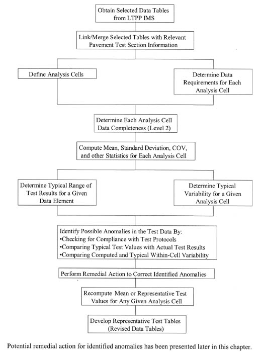
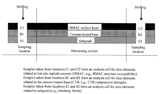
Level 1--Data Completeness
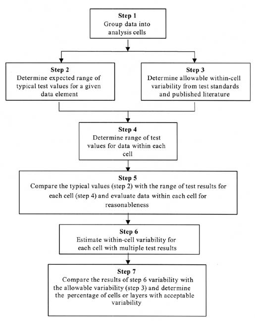
Cell Type (layer 1, SHRP_ID 001) Number of Specimens Mean Thickness, mm Target Thickness, mm1 Min Thickness Range, mm Max Thickness Range, mm GPS-XX
GPS-XX
SPS-XX
SPS-XX
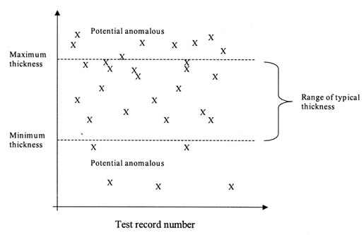
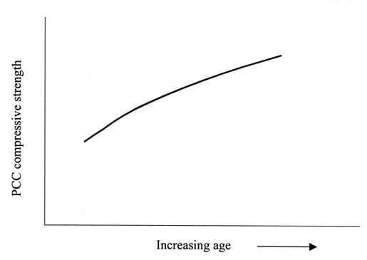
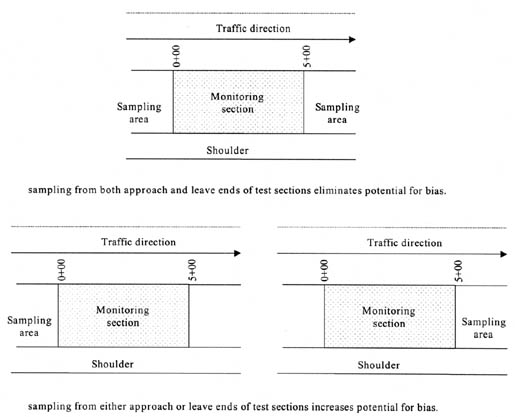
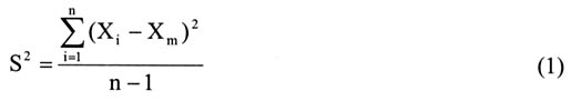
Xi = Test result from the ith specimen
Xm = Sample mean
S = Sample standard deviation
n = Number of specimens 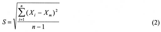
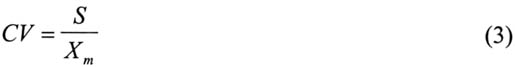
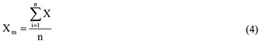
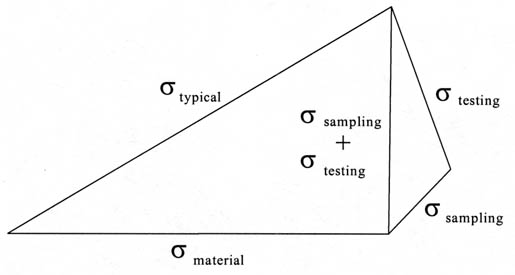

sigmaST = Variability due to sampling and testing
sigmaS = Sampling variability
sigmaT = Testing variability![]()
sigmaTYP = Typical variability
sigmaST = Variability due to sampling and testing
sigmaM = Material variability
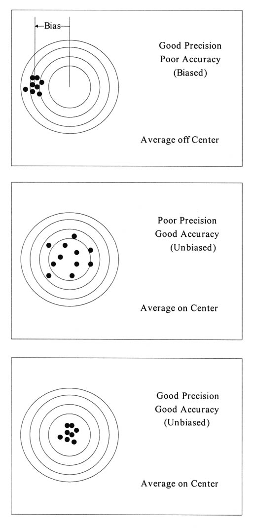
Identified Anomaly Effect on Data Quality Recommended Remedial Action Insufficient data at level E due to test results still undergoing QA/QC at levels A to D Data are inadequate for analysis (data might not represent test section) Upgrade representative data tables when QA/QC process is complete
Insufficient data at level E due to insufficient testing and/or test results failing QA/QC checks between levels A to D Data are inadequate for analysis (data might not represent test section) Adopt representative values from similar sections
Insufficient data at level E due to insufficient testing and/or test results failing QA/QC checks between levels A to D Data are inadequate for analysis (data might not represent test section) Backcast or forecast from time-series data
Insufficient data at level E due to insufficient testing and/or test results failing QA/QC checks between levels A to D Data are inadequate for analysis (data might not represent test section) Estimate data from analytical models or techniques
Inadequate sampling (e.g., single test values) Possible bias due to unrepresentative test values Check sampling locations to verify that the data adequately represent test section
Inadequate sampling (e.g., single test values) Possible bias due to unrepresentative test values Resampling and testing to obtain more representative test results
Noncompliance with testing protocol Excessive variability in multiple test results (assuming only a few of the test values are noncompliant) Identify individual noncompliant test values as potential outliers and study their effect on variability
Noncompliance with testing protocol Potential for systematic bias if all tests on multiple specimens are noncompliant. Perform forensic testing
Unreasonable multiple test values Excessive variability in multiple test results (assuming only a few of the test values are unreasonable) Identify individual unreasonable test values as potential outliers and study their effect on variability. Remove outliers from developing representative data tables if they are the cause of the excessive variability
Unreasonable single test values Unreliable data Perform forensic testing
Unexplained excessive variability Unreliable data Identify potential outliers and errors using statistical techniques (ASTM E178)
Missing experiment type and layer information -- Consult materials testing and construction data sheets or other data tables with the database to determine the required information
Missing specimen testing age or anomalous computed ages -- Consult materials testing and construction data sheets or other data tables with the database to determine the required information
Experiment Type Layer Type LTPP Designation SHRP Protocol Minimum Number of Tests per Layer Sampling Location GPS 1, 2, 6, and 7 AC AC01 P01 16 All 100-mm and 150-mm-diameter cores
SPS-1 Asphalt treated base AC01 P01 34 102-mm OD coresC1-C10, C21-C34,C47-C56
SPS-1 AC surface and binder AC01 P01 60 102-mm OD coresC1-C60
SPS-3 Asphalt treated base AC01 P01 34 102-mm OD coresC1-C10, C21-C34,C47-C56
SPS-3 AC surface and binder AC01 P01 60 102-mm OD coresC1-C60
SPS-5 Preconstruction AC AC01 P01 26 All Type-C cores
SPS-5 Postconstruction AC AC01 P01 40 All cores
SPS-6 AC AC01 P01 20 All cores
SPS-8 AC AC01 P01 16 All cores
SPS-9 Preconstruction AC AC01 P01 6 A01A01,A02A01,A01A02A02A02,A01A03,A02A03
SPS-9 Postconstruction AC AC01 P01 8 --
Experiment Type Test Section Material Description Min. No. of Cores Required(Surface and binder/ATB) Sampling Location SPS-1 0101 (0113) AC 6/0 C41-C46
SPS-1 0102 (0114) AC 4/0 C57-C60
SPS-1 0103 (0115) AC 4/4 C47-C50
SPS-1 0104 (0116) AC 4/4 C1-C4
SPS-1 0105 (0117) AC 6/6 C51-C56
SPS-1 0106 (0118) AC 6/6 C5-C9
SPS-1 0107 (0119) AC 6/0 C35-C40
SPS-1 0108 (0120) AC 6/0 C15-C20
SPS-1 0109 (0121) AC 4/0 C11-C14
SPS-1 0110 (0122) AC 4/4 C21-C24
SPS-1 0111 (0123) AC 4/4 C31-C34
SPS-1 0112 (0124) AC 6/4 C25-C30
SPS-5 (Preconstruction) 0501 AC 2 C1,C2
SPS-5 (Preconstruction) 0502 AC 4 C3-C6
SPS-5 (Preconstruction) 0503 AC 2 C7-C8
SPS-5 (Preconstruction) 0504 AC 2 C9-C10
SPS-5 (Preconstruction) 0505 AC 2 C11-C12
SPS-5 (Preconstruction) 0506 AC 5 C13-C17
SPS-5 (Preconstruction) 0507 AC 2 C18-C19
SPS-5 (Preconstruction) 0508 AC 5 C20-C24
SPS-5 (Preconstruction) 0509 AC 2 C25-C26
SPS-5 (Postconstruction) 0501 AC 0 --
SPS-5 (Postconstruction) 0502 AC 4 C27-C30
SPS-5 (Postconstruction) 0503 AC 6 C31-C35
SPS-5 (Postconstruction) 0504 AC 6 C37-C42
SPS-5 (Postconstruction) 0505 AC 4 C43-C46
SPS-5 (Postconstruction) 0506 AC 4 C47-C50
SPS-5 (Postconstruction) 0507 AC 6 C51-C56
SPS-5 (Postconstruction) 0508 AC 6 C57-C62
SPS-5 (Postconstruction) 0509 AC 4 C63-C66
SPS-6 (Preconstruction) 0601 AC 3 C1-C3
SPS-6 (Preconstruction) 0602 AC 3 C3-C6
SPS-6 (Preconstruction) 0603 AC 2 C11-C12
SPS-6 (Preconstruction) 0604 AC 2 C13-C14
SPS-6 (Preconstruction) 0605 AC 4 C7-C10
SPS-6 (Preconstruction) 0606 AC 2 C15-C16
SPS-6 (Preconstruction) 0607 AC 2 C17-C18
SPS-6 (Preconstruction) 0608 AC 2 C19-C20
SPS-6 (Postconstruction) 0603 AC 4 C21-C24
SPS-6 (Postconstruction) 0604 AC 4 C25-C28
SPS-6 (Postconstruction) 0606 AC 4 C29-C32
SPS-6 (Postconstruction) 0607 AC 4 C33-C36
SPS-6 (Postconstruction) 0608 AC 4 C37-C40
SPS-8 0801, 0803, 0805 AC 8 C1-C8
SPS-8 0802, 0804, 0806 AC 8 C9-C16
SPS-9 0901, 0902, 0903 AC 8 --
Data Fields GPS SPS SHRP_ID X X
State Cored X X
Layer number X X
Construction number X X
Experiment Type Expt. Number Total Number of Records at All Levels Total Number of Records at Level E Percentage of Records at Level E Number of Analysis Cells Represented at Level E GPS 1 8069 8067 99.6 488
GPS 2 5655 5655 100 349
GPS 3 159 159 100 13
GPS 4 30 30 100 2
GPS 5 275 275 100 22
GPS 6A 3496 3496 100 218
GPS 6B 3359 3359 100 189
GPS 6C 505 500 99 35
GPS 6D 128 128 100 9
GPS 6S 1584 1561 99 104
GPS 7A 1185 1183 99.8 72
GPS 7B 529 529 100 29
GPS 7C 36 36 100 2
GPS 7S 189 189 100 8
GPS 9 322 312 96.9 27
SPS 1 1977 1965 99.4 423
SPS 3 1928 1928 100 958
SPS 5 2577 2550 99 568
SPS 6 248 248 100 64
SPS 8 237 237 100 31
SPS 9 625 559 89.4 52
Experiment Type Number of Analysis Cells with Data Min. Number of Test Results Required Analysis Cells with Minimum Number of Test Results Percentage Analysis Cells with Minimum Test Results GPS-1 459 16 392 85.4
GPS-2 340 16 291 85.6
GPS-6A 212 16 186 87.7
GPS-6B 182 16 141 77.5
GPS-6C 30 16 16 53.3
GPS-6D 8 16 3 37.5
GPS-6S 79 16 38 48.1
GPS-7A 65 16 48 73.9
GPS-7B 27 16 18 66.7
GPS-7C 2 16 2 100
GPS-7S 8 16 8 100
SPS-1 228 5/31 135 59.2
SPS-3 914 3 138 15.1
SPS-5 471 3/42 311 66.0
SPS-6 39 2 36 2.3
SPS-8 21 4 21 100
2For each section in the SPS-5 project, three tests are required on the original AC surface preconstruction, and four tests are required on the overlay postconstruction.
LTPP Layer Description Code Number Material/Layer Description Typical Thickness Range, mm No. of Test Records With Thickness within Range No. of Analysis Cells With Thickness within Range Number of Test Records out of range 1 Overlay 12.5 - 150 3848 228 26
2 Seal coat 2.5 - 37.5 1836 115 35
3 Original surface 12.5 - 325 7830 474 72
4 AC layer below surface 12.5 - 250 5712 368 99
5 Base 25 - 600 1253 86 12
6 Subbase 75 - 1200 30 2 0
8 Interlayer 2.5 - 150 574 40 0
9 Friction course 2.5 - 62.5 1838 112 0
10 Surface treatment 2.5 - 37.5 77 5 0
Expt. Type Layer Description Target Thickness, mm Number of Core Specimens Mean Thickness, mm Standard Deviation, mm COV, percent Min. Thickness Range, mm Max. Thickness Range, mm GPS Overlay 12.5 - 150 3874 54.7 27 49.4 2.5 191
GPS Seal coat 2.5 - 37.5 1871 9.3 10 108.0 2.5 97
GPS Original surface 12.5 - 325 7962 68 51 74.6 5.1 401
GPS AC layer below surface 12.5 - 250 5838 88 61 68.9 25 406
GPS Base 25 - 600 1263 142 66 46.4 51 363
GPS Subbase 75 - 1200 30 101 10 10.0 86 127
GPS Interlayer 2.5 - 150 574 25 28 113.4 2.5 109
GPS Friction course 2.5 - 62.5 1838 17 12 66.6 2.5 69
GPS Surface treatment 2.5 - 37.5 77 3.4 2.2 63.6 2.5 10
SPS-1 Surface 102 50 106.5 18.2 17.1 53 147
SPS-1 Surface 178 45 168.2 32.3 16.5 41 201
SPS-5 Overlay 51 45 74.3 23.7 31.9 42 119
SPS-5 Overlay 127 48 150.1 25.6 17.1 114 200
SPS-6 Overlay 102 16 103.7 9.0 8.7 86 120
SPS-6 Overlay 203 4 210.0 7.4 3.5 199 215
SPS-8 Surface 102 7 105.3 10.5 10.0 91 119
SPS-8 Surface 178 7 171.2 15.7 9.2 142 187
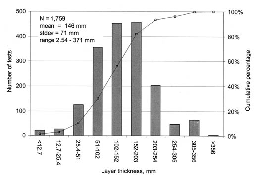
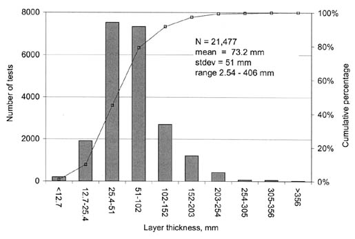
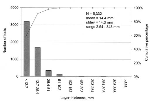
Data Source Layer Type Average Thickness, mm Standard Deviation, mm COV, percent New Jersey Surface 44 6.6 15.0
New Jersey Surface/binder 57 8.4 14.7
New Jersey Surface/binder 85 10.6 12.5
New Jersey Base 100 14.0 14.0
New Jersey Base 150 14.0 9.3
Kansas DOT1 Surface/base 112 5.6 5.0
Kansas DOT1 Surface/base 71 6.6 9.3
Kansas DOT1 Surface/base 487 19.3 4.0
Kansas DOT1 Surface/base 67 5.6 8.4
Kansas DOT1 Surface/base 188 22.1 11.7
Kansas DOT1 Surface/base 356 6.1 1.7
Kansas DOT1 Surface/base 272 26.4 9.7
Kansas DOT1 Surface/base 319 22.6 7.1
Average COV, percent, 9.4
1Consists of core for binder, surface layer, and base layers.
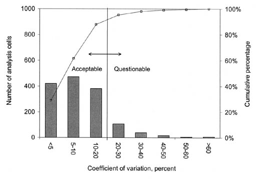
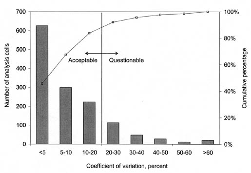
Data Fields GPS SPS1 SHRP_ID X X
State code X X
Layer number X X
Layer description X
Material code X
Experiment Type Layer Type LTPP Designation SHRP Protocol Minimum Number of Tests per Layer Sampling Location GPS-1, -2, -6, and -7 AC AC02 P02 2 A1, A2, C7, C9, C10, C19, C21, C22, (C12, C24 if needed)
Expt Type Construction Stage LTPP Designation Sections Minimum Number of Tests per Layer Source/Sampling Location SPS-1 Asphalt-treated base AC02 -- 34 102-mm OD cores C1-C10, C21-C34, C47-C56
SPS-1 AC surface and binder AC02 -- 60 102-mm OD coresC1-C60
SPS-5 Preconstruction AC02 -- 9 C3, C4, C5, [C13,C14,C15], [C22,C23,C24]
SPS-5 Postconstruction AC02 -- 40 All cores
SPS-6 -- AC02 -- 20 All cores
SPS-8 -- AC02 -- 16 All cores
SPS-9 Mix design AC02 01 and 03 3 LA01AXX-LA03AXX
SPS-9 Compacted bulk samples AC02 02 18 LA01A02-LA07LA02, LA15A02, LA38A02, DA02A02,DA03A02, DA04A02, DA06A02, DA16A02, DA22A02, DA31A02, DA32A02, DA33A02
SPS-9 QA test AC02 01 and 03 6 BA01AXX-BA06AXX
Postconstruction AC02 01, 02, and 03 8 CA02tXX, CA06tXX, CA11txx, CA15txx, CA19tXX, CA24tXX, CA28tXX, CA33tXX
Experiment Type Experiment No. Total Number of Records at All Levels Total Number of Records at at Level E Percentage of Records at Level E Number of Analysis Cells Represented at Level E GPS 1 1831 1829 99.89 320
GPS 2 1472 1470 99.86 239
GPS 3 40 40 100 10
GPS 4 6 6 100 2
GPS 5 89 89 100 23
GPS 6A 780 779 99.87 138
GPS 6B 385 378 98.18 92
GPS 6C 28 28 100 6
GPS 6D 12 11 91.67 2
GPS 6S 174 172 98.85 40
GPS 7A 226 226 100 49
GPS 7B 125 125 100 24
GPS 7C 16 16 100 2
GPS 7S 8 8 100 4
GPS 9 22 22 100 7
SPS 1 1035 1010 97.6 42
SPS 5 1190 1079 90.7 54
SPS 6 186 130 69.9 9
SPS 8 100 100 100 9
SPS 9 299 256 85.6 11
Experiment Type No. of Analysis Cells with Data Min. Number of Test Results Required No. of Analysis Cells with Min. Number of Test Results Percent Analysis Cells with Minimum Test Results GPS-1 298 2 293 98.3
GPS-2 234 2 229 97.9
GPS-3 10 2 8 80.0
GPS-4 1 2 1 100
GPS-5 23 2 23 100
GPS-6A 135 2 129 95.6
GPS-6B 92 2 79 85.9
GPS-6C 6 2 6 100
GPS-6D 2 2 1 50.0
GPS-6S 33 2 30 90.9
GPS-7A 45 2 44 97.8
GPS-7B 22 2 22 100
GPS-7C 2 2 2 100
GPS-7S 4 2 4 100
GPS-9 4 2 4 100
SPS-11 24 60/34 2 8.3
SPS-52 60 9/40 13 22.0
SPS-6 7 20 3 43.0
SPS-8 6 16 3 50.0
2For the SPS-5 project, nine tests are required on the original AC surface preconstruction, and 40 tests are required on the overlay postconstruction.
Type of Rock Specific Gravity Absorption (percent) Granite 2.65 0.3
Syenite 2.74 0.4
Diorite 2.92 0.3
Felsite 2.66 1.8
Limestone 2.66 0.9
Dolomite 2.70 1.1
Shale 1.8-2.5 > 1.0
Sandstone 2.54 1.8
SHRP_ID BSG Possible Anomaly 481119 3.347 Higher than typical test values
481119 3.402 Higher than typical test values
491005 0.49 Lower than typical test values
483669 1.617 Lower than typical test values
483669 1.734 Lower than typical test values
483679 1.554 Lower than typical test values
483679 1.580 Lower than typical test values
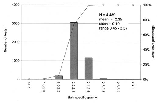
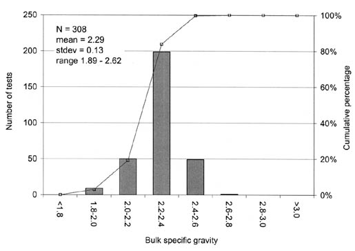
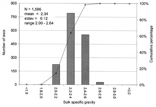
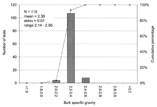

MSG = maximum specific gravity
BSG = bulk specific gravity
Data Source Method Standard Deviation, percent California Cores 1.9
New Jersey Cores 1.5
Ontario Cores 1.6
Colorado Cores 1.0
Washington Nuclear 0.9
Virginia Cores 1.3
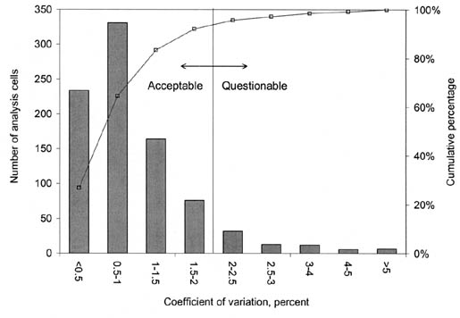
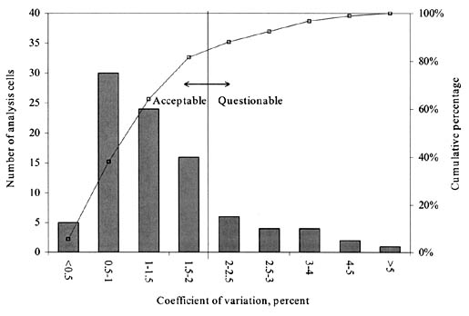
Number TST_AC02_REP_GPS TST_AC02_REP_SPS 1 State code State code
2 SHRP identification number SPS cell identification number
3 Layer number Description of Layer
4 Construction number Material code for the layer
5 Number of specimen tested Construction number
6 Mean BSG Number of specimen tested
7 Maximum BSG Mean BSG
8 Minimum BSG Maximum BSG
9 Standard deviation of BSG data Minimum BSG
10 COV of BSG data COV of BSG data
11 QA_Comment_1 Standard deviation of BSG data
12 QA_Comment_2 QA_Comment_1
13 QA_Comment_3 QA_Comment_2
14 QA_Comment_4 QA_Comment_3
15 QA_Comment_5 QA_Comment_4
16 QA_Comment_6 QA_Comment_5
17 QA_Comment_Other QA_Comment_6
18 Record status QA_Comment_Other
19 -- Record status
1SPS 1, 2, 5, 6, 7, 8, and 9A.Data Fields GPS SPS1 SHRP_ID X X
State code X X
Layer number X X
Layer description X
Material code X
Expt. Type Layer Type LTPP Designation SHRP Protocol Minimum Number of Tests per Layer Sampling Location GPS-1, -2, -6, and -7 AC AC03 P03 2 A1, A2
Note: Postconstruction cores to be tested at 0, 6, 12, 18, 24, and 48 months after construction.Expt. Type Construction Stage SHRP Protocol Sections Minimum Number of Tests per Layer Source/Location SPS-1 Asphalt-treated base P03 -- 3 B19, B20, B21from paver
SPS-1 AC surface and binder layer P03 -- 3 B25, B26, B27from paver
SPS-5 Preconstruction P03 -- 3 BA1-3, TP, BA4-6
SPS-5 Postconstruction P03 -- 6 BV1, BV2, BV3, BR1, BR2, BR3
SPS-6 -- P03 -- 3 BV1, BV2, BV3,
SPS-8 -- P03 -- 3 BV-01, BV-02, BV-03,
SPS-9 Mix design P03 01 and 03 1 NA01AXX
SPS-9 Compacted bulk samples P03 02 3 NA15A02, BA06A02, BA22A02
SPS-9 QA test P03 01 and 03 2 BA02AXX BA04AXX
SPS-9 Postconstruction P03 01, 02, and 03 8 CA02tXX, CA06tXX, CA11txx, CA15txx, CA19tXX, CA24tXX, CA28tXX, CA33tXX
Expt Type Expt Number Total Number of Records at All Levels Total Number of Records at Level E Percentage of Records at Level E Number of Analysis Cells Represented at Level E GPS 1 610 608 99.70 306
GPS 2 609 607 99.70 213
GPS 3 6 6 100.00 4
GPS 4 2 2 100.00 1
GPS 6A 257 256 99.60 129
GPS 6B 162 159 98.10 85
GPS 6C 10 10 100.00 5
GPS 6D 4 3 75.00 2
GPS 6S 63 61 96.80 32
GPS 7A 123 123 100.00 49
GPS 7B 52 50 96.20 24
GPS 7C 2 2 100.00 1
GPS 7S 8 8 100.00 4
GPS 9 14 14 100.00 7
SPS 1 124 124 100.00 35
SPS 2 6 6 100.00 1
SPS 5 174 174 100.00 42
SPS 6 66 10 15.20 4
SPS 8 21 21 100.00 9
SPS 9 45 41 91.10 9
1NR -- Not required by the materials testing plan.Experiment Type No. of Analysis Cells with Test Data and Material Information Min. Number of Test Results Required Analysis Cells with Minimum Number of Test Results Percent Analysis Cells with Minimum Test Results GPS-1 289 2 269 93.10
GPS-2 209 2 200 95.70
GPS-3 4 2 2 50.00
GPS-6A 126 2 118 93.70
GPS-6B 85 2 72 84.70
GPS-6C 5 2 5 100.00
GPS-6D 2 2 1 50.00
GPS-6S 25 2 23 92.00
GPS-7A 45 2 42 93.30
GPS-7B 23 2 23 100.00
GPS-7C 1 2 1 100.00
GPS-7S 4 2 4 100.00
GPS-9 4 2 4 100.00
SPS-1 20 3 18 90.00
SPS-2 1 NR1 1 100.00
SPS-5 39 3/62 10 26.00
SPS-6 3 3 1 33.00
SPS-8 5 3 2 40.00
2For the SPS-5 project three tests are required on the original AC surface preconstruction, and six tests are required on the overlay postconstruction.
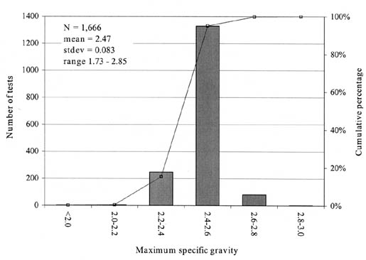
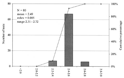
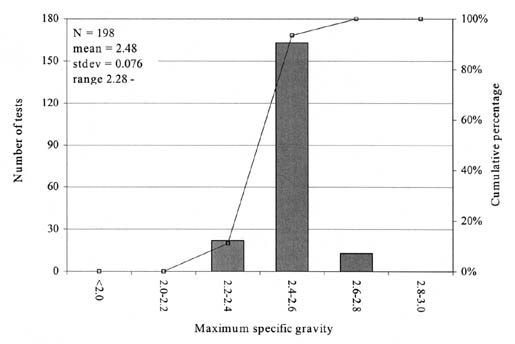
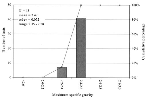
Condition of Test Standard Deviation Acceptable Range for Two Test Results Single operator (not based on the use of section 7 of AASHTO T209)1 0.0004 0.011
Multiple operator (not based on the use of section 7 of AASHTO T209)1 0.00064 0.019
Single operator (based on the use of section 7 of AASHTO T209)2 0.00064 0.018
Multiple operator (based on the use of section 7 of AASHTO T209)2 0.0193 0.055
2Basis of estimate: two replicates, seven materials, and ten laboratories.
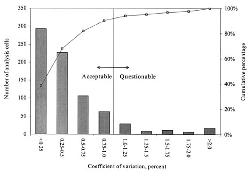
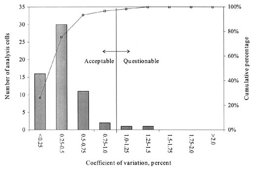
Number GPS SPS 1 State code State code
2 SHRP identification number SPS cell identification number
3 Layer number Description of layer
4 Construction number Material code for the layer
5 Number of specimen tested Construction number
6 Mean MSG Number of specimen tested
7 Maximum MSG Mean MSG
8 Minimum MSG Maximum MSG
9 Standard deviation Minimum MSG
10 COV COV
11 QA_Comment_1 Standard deviation
12 QA_Comment_2 QA_Comment_1
13 QA_Comment_3 QA_Comment_2
14 QA_Comment_4 QA_Comment_3
15 QA_Comment_5 QA_Comment_4
16 QA_Comment_6 QA_Comment_5
17 QA_Comment_Other QA_Comment_6
18 Record status QA_Comment_Other
19 -- Record status
Expt. Type Layer Type SHRP Protocol Minimum Number of Tests per Layer Sampling Location GPS-1, -2, -6, and -7 AC P04 2 TP, BA1
Expt Type Construction Stage SHRP Protocol Sections Min. No. of Tests per Layer Source/Location SPS-1 Asphalt-treated base P04 -- 3 B19, B20, B21from paver
SPS-1 AC surface and binder layer P04 -- 3 B25, B26, B27from paver
SPS-2 Asphalt-treated base P04 -- 3 B16 to B18from paver
SPS-5 Preconstrution P04 -- 3 BA1-3, TP, BA4-6
SPS-5 Postconstrution P04 -- 6 BV1, BV2, BV3, BR1, BR2, BR3
SPS-6 -- P04 -- 3 BV1, BV2, BV3,
SPS-8 -- P04 -- 3 BV-01, BV-02, BV-03,
SPS-9 Mix design P04 01 and 03 0 --
SPS-9 Compacted bulk samples P04 02 6 BA01A02, BA06A02, BA11A02, BA16A02, BA22A02, BA34A02
QA test P04 01 and 03 2 BA02AXX-BA04AXX
SPS-9 Post construction P04 01, 02, and 03 8 CA02tXX, CA06tXX, CA11txx, CA15txx, CA19tXX, CA24tXX, CA28tXX, CA33tXX
1SPS-1, -2, -5, -6, -7, -8, and -9A.Key Fields GPS SPS1 SHRP_ID X X
State code X X
Layer number X X
Construction number X X
Layer type X
Material code X
Expt Type Expt Number Total Number of Records at All Levels Total Number of Records at Level E Percentage of Records at Level E Number of Analysis Cells Represented at Level E GPS 1 602 599 99.50 302
GPS 2 607 607 100.00 214
GPS 3 5 5 100.00 3
GPS 4 2 2 100.00 1
GPS 6A 262 261 99.60 133
GPS 6B 189 187 98.90 84
GPS 6C 16 16 100.00 6
GPS 6D 4 3 75.00 2
GPS 6S 77 77 100.00 23
GPS 7A 118 118 100.00 49
GPS 7B 52 49 94.20 23
GPS 7C 2 2 100.00 1
GPS 7S 12 12 100.00 4
GPS 9 12 12 100.00 7
SPS 1 141 136 96.50 42
SPS 2 28 28 100.00 12
SPS 5 181 181 100.00 40
SPS 6 6 6 100.00 3
SPS 8 21 21 100.00 9
SPS 9A 125 125 100.00 10
Expt. Type No. of Analysis Cells with Test Data and Material Information Min. Number of Test Results Required Analysis Cells with Minimum Number of Test Results Percent Analysis Cells with Minimum Test Results GPS-1 288 2 271 94.10
GPS-2 208 2 201 96.60
GPS-3 3 2 2 66.70
GPS-6A 129 2 126 97.70
GPS-6B 84 2 74 88.10
GPS-6C 6 2 6 100.00
GPS-6D 2 2 1 50.00
GPS-6S 18 2 18 100.00
GPS-7A 45 2 41 1.10
GPS-7B 22 2 21 95.50
GPS-7C 1 2 1 100.00
GPS-7S 4 2 4 100.00
GPS-9 4 2 2 50.00
SPS-1 31 3 23 74.00
SPS-2 7 NR1 6 86.00
SPS-5 36 3/62 11 31.00
SPS-6 3 3 1 33.00
SPS-8 5 3 2 40.00
2For the SPS-5 projects, three tests are required on the original AC surface preconstruction, and six tests are required on the overlay postconstruction.
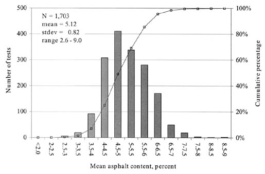
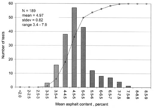
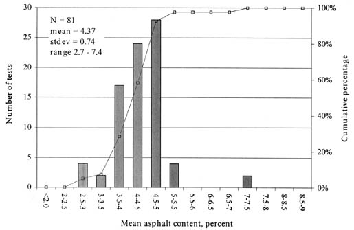
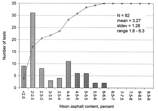
Data Source Year Test Method Standard Deviation, percent Virginia 1994 Extraction 0.18
Virginia 1994 Nuclear 0.21
NCAT 1994 Nuclear 0.19
NCAT 1994 Centrifuge 0.44
Washington 1993 Extraction 0.24
Colorado 1993 Extraction 0.15
Pennsylvania 1980 Extraction 0.25
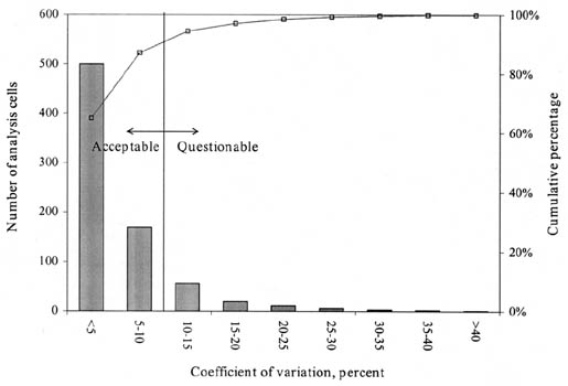
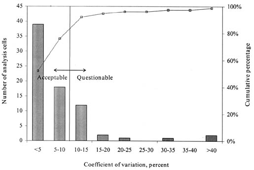
Number GPS SPS 1 State code State code
2 SHRP identification number SPS cell identification number
3 Layer number Description of layer
4 Construction number Material code for the layer
5 Number of specimen tested Construction number
6 Mean asphalt content Number of specimen tested
7 Maximum asphalt content Mean asphalt content
8 Minimum asphalt content Maximum asphalt content
9 Standard deviation of asphalt content Minimum asphalt content
10 COV of asphalt content COV of asphalt content
11 QA_Comment_1 Standard deviation of asphalt content
12 QA_Comment_2 QA_Comment_1
13 QA_Comment_3 QA_Comment_2
14 QA_Comment_4 QA_Comment_3
15 QA_Comment_5 QA_Comment_4
16 QA_Comment_6 QA_Comment_5
17 QA_Comment_Other QA_Comment_6
18 Record status QA_Comment_Other
19 -- Record status

Experiment Type Layer Type LTPP Designation SHRP Protocol Minimum Number of Tests per Layer Sampling Location SPS-1 Asphalt treated base AC05 P05 3 B19, B20, B21 from paver
SPS-1 AC surface and binder AC05 P05 3 B25, B26, B27from paver
SPS-5 (Postconstruction) AC AC05 P05 6 BV1, BV2, BV3, BR1, BR2, BR3
SPS-6 AC AC05 P05 3 BV1, BV2, BV3,
SPS-8 AC AC05 P05 3 BV-01, BV-02, BV-03,
Information in this table was used to define analysis cells for data evaluation (i.e., unique combination of State_Code, SHRP_ID, and Material_Code). Table 36 presents the fields used in defining analysis cells for the various SPS experiments.
1SPS-1, -2, -5, -6, -7, -8, and -9AKey fields GPS SPS1 SHRP_ID X X
State code X X
Layer number X X
Construction number X X
Layer type X
Material code X
Expt. Type Expt. Number Total Number of Records at All Levels Total Number of Records at Level E Percentage of Records at Level E Number of Analysis Cells Represented at Level E GPS 6S 2 -- -- --
SPS-1 1 57 33 57.9 13
SPS-5 5 32 21 65.6 7
SPS-8 8 22 9 40.9 3
Expt. Type No. of Analysis Cells with Test Data and Material Information Min. Number of Test Results Required Analysis Cells with Minimum Number of Test Results Percent Analysis Cells with Minimum Test Results SPS-1 6 3 4 67
SPS-5 3 6 0 0
SPS-8 2 3 2 100
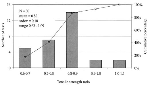
3Feedback reports enable users of the LTPP database to report any situations encountered during FHWA-sponsored data analysis that suggest or demonstrate the need for corrective actions or further investigation. Such situations include, but are not limited to:
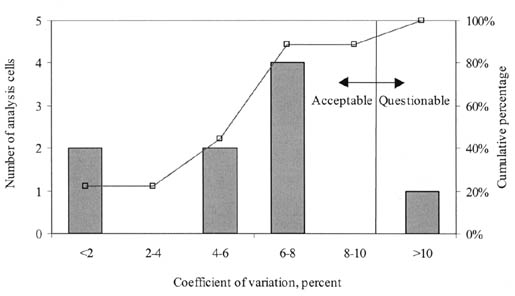
Expt. Type Expt. No. No. of Records at Levels A to E No. of Records at Level E No. of Usable Records at Level E Percent Usable Records at Level E Total Number of Analysis Cells Represented GPS 3 824 818 8181 99 123
GPS 4 440 436 4362 99 61
GPS 5 545 540 5403 99 81
GPS 7A 330 330 3244 98 35
GPS 7B 67 67 605 90 7
GPS 9 331 331 3246 98 48
SPS 1 26 0 0 0 --
SPS 2 1354 1121 9907 73 116--PCC
36--LCBSPS 6 231 168 168 73 51
SPS 7 552 536 5028 91 25--Original
28--OverlaySPS 8 16 16 16 100 2
SPS 9 170 82 309 18 2
2Four records are missing thickness information.
3Five records are missing thickness information.
4Six records are missing thickness information.
5Two records are missing thickness information; five records have discrepancies in material type descriptions.
6One record is missing thickness information; six records do not have corresponding L05B information.
7Eighty-eight records do not have corresponding L05B information; 41 records are missing thickness information; 2 records have discrepancies in material type descriptions.
8Eleven records do not have corresponding L05B information; 23 records are missing thickness information.
9Fifty-two records pertaining to supplemental sections are present at level E.
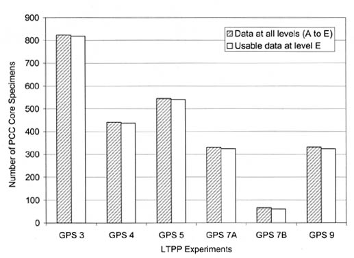
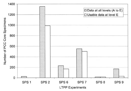
Key Fields GPS Experiments (All) SPS Experiments (All) Experiment type X X
Experiment number X X
SHRP_ID X X
State code X X
Construction number X X
Layer number X X
Material code X X
Experiment Type Layer Type Test Type LTPP Designation LTPP Protocol Minimum Number of Tests per Layer Sampling Location1 GPS-3, 4, 5, & 9 PCC Core examination and thickness PC06 P66-61 2 C2, C8
GPS-7 PCC Core examination and thickness PC06 P66-61 2 C8, C20
GPS-3, 4, 5 & 9 PCC Core examination and thickness PC06 P66-62 2 C5, C11
GPS-7 PCC Core examination and thickness PC06 P66-62 2 C11, C23
GPS-3, 4, 5 & 9 PCC Core examination and thickness PC06 P66-64 2 C1, C7
GPS-7 PCC Core examination and thickness PC06 P66-64 2 C7, C19
SPS-2 PCC Core examination and thickness PC06 P66 99 per site/project All cores
SPS-2 LCB Core examination and thickness PC06 P66 24 per site/project --
SPS-6 PCC Core examination and thickness PC06 P66 23 per site/project C1-C20 A1 A2 A3
SPS-7 PCC--overlay (postconstruction) Core examination and thickness PC06 P66 99 per site/project C10-20 C21-64 C65-108
SPS-7 PCC--overlay (preconstruction) Core examination and thickness PC06 P66 47 per site/porject C10-20 C21-64 C65-108
SPS-8 PCC Core examination and thickness PC06 P66 26 per site/project C1-C26
SPS-9A PCC Core examination and thickness PC06 P66 6 per site/project --
Experiment Type Test Section Layer Type Min. No. of Specimens Required per Layer Sampling Location1 SPS-2 201 (215) PCC 8 C10-C17
SPS-2 202 (216) PCC 8 C59-C66
SPS-2 203 (213) PCC 9 C34-C42
SPS-2 204 (214) PCC 8 C83-C90
SPS-2 205 (219) PCC 8 C21-C25C18-C20, C22-C24
SPS-2 206 (220) PCC 8 C73-C74C67-C72
SPS-2 207 (217) PCC 8 C29-C33C26-C28, C30-C32
SPS-2 208 (218) PCC 8 C78, C82C75-C77, C79-C81
SPS-2 209 (223) PCC 9 C1-C9
SPS-2 210 (224) PCC 8 C51-C58
SPS-2 211 (221) PCC 8 C43-C50
SPS-2 212 (222) PCC 9 C91-C99
SPS-2 205 (219) LCB 6 C18-C20, C22-C24
SPS-2 206 (220) LCB 6 C67-C72
SPS-2 207 (217) LCB 6 C26-C28, C30-C32
SPS-2 208 (218) LCB 6 C75-C77, C79-C81
SPS-6 601 Original PCC 3 C1-C3
SPS-6 602 Original PCC 4 C4-C6, A1
SPS-6 603 Original PCC 3 C11-C12
SPS-6 604 Original PCC 2 C13-C14
SPS-6 605 Original PCC 4 C7-C10
SPS-6 606 Original PCC 2 C15-C16
SPS-6 607 Original PCC 3 C17-C18, A3
SPS-6 608 Original PCC 2 C19-C20
SPS-7 701 Original (Overlay) 1 (0) A1
SPS-7 702 Original (Overlay) 1 (8) A2 (C21-C24, C65-C68)
SPS-7 703 Original (Overlay) 3 (9) C1-C3 (C10, C25-C28, C69-C72)
SPS-7 704 Original (Overlay) 1 (8) A3 (C29-C32, C73-C76)
SPS-7 705 Original (Overlay) 4 (8) A4, BA1-BA3 (C33-C36, C77-C80)
SPS-7 706 Original (Overlay) 3 (11) C4-C6 (C11-C13, C37-C40, C81-C84)
SPS-7 707 Original (Overlay) 1 (17) A5 (C14-C16, C44-C50, C88-C94)
SPS-7 708 Original (Overlay) 1 (16) A6 (C17-C18, C51-C57, C95-C101)
SPS-7 709 Original (Overlay) 3 (16) C7-C9 (C19-C20, C58-C64, C102-C108)
SPS-8 807, 809, 811 Overlay 13 C1-C13
SPS-8 808, 810, 812 Overlay 13 C14-C26
SPS-9A 901, 902, 903 Original 2 --
Experiment Type Layer Type Total Number of Cells Number of Cells with Less Than Minimum Number of Tests Percent Cells with Incomplete Data GPS-3 PCC original 123 0 0
GPS-4 PCC original 61 0 0
GPS-5 PCC original 81 0 0
GPS-7A PCC original 35 0 0
GPS-7B PCC original 7 1
(1 single test value)14
GPS-9 PCC original 48 0 0
SPS-2 PCC 116 60
(1 single test value)52
SPS-2 LCB 36 12
(1 single test value)33
SPS-6 PCC 51 12
(5 single test values)24
SPS-7 PCC original 25 5
(2 single test values)20
SPS-7 PCC overlay 28 28
(1 single test value)100
SPS-8 PCC 2 2 100
SPS-9A PCC 6 0 0
Experiment Type Target Thickness, mm Number of Specimens Mean Thickness, mm Standard Deviation, mm1 COV, percent1 Min Thickness Range, mm Max Thickness Range, mm GPS-3 -- 818 240.9 31.6 13.1 152.4 370.8
GPS-4 -- 436 240.2 20.9 8.7 190.5 302.3
GPS-5 -- 540 221.8 27.5 12.4 154.9 335.3
GPS-7A -- 324 215.6 22.4 10.4 165.1 261.6
GPS-7B -- 60 225.1 23.7 10.5 190.5 271.8
GPS-9 -- 324 218.6 25.2 11.5 165.1 335.3
SPS-2 (203-mm sections) 203.2 414 211.5 17.3 8.2 127.0 287.0
SPS-2 (279-mm sections) 279.4 390 277.8 28.5 10.3 129.0 325.1
SPS-2 (sections with LCB) 152.4 186 162.4 14.8 9.1 120.9 213.4
SPS-6 -- 168 232.4 17.1 7.4 198.1 266.7
SPS-7 (original PCC layer) -- 203 192.5 29.9 15.6 53.3 218.4
SPS-7 (75-mm overlay sections) 76.2 114 164.4 91.3 55.5 74.7 307.3
SPS-7 (125-mm overlay sections) 127.0 185 166.8 64.8 38.8 101.6 353.1
SPS-8 (200-mm sections) 203.2 9 193.0 6.7 3.5 183.4 200.7
SPS-8 (275-mm sections) 279.4 7 283.1 5.8 2.1 278.4 294.1
SPS-9 -- 30 227.4 13.6 6.0 203.2 246.4
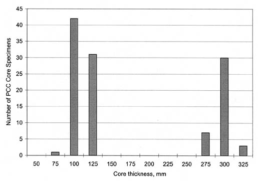
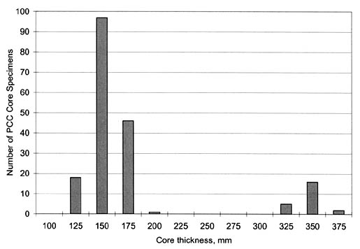
Data Item Reference Specimen Type COV, percent Standard Deviation PCC Thickness Terzaghi et al.(24)
PCC Thickness SHRP SPS-2(25) Cores 2 to 31
PCC Thickness Yoder and Witzak(26) Cores 2.5 to 12.5 mm
PCC Thickness Darter(27) Cores 3.1 to 3.2 8 mm
PCC Thickness Hoerner et al.(28) Cores 3.3 8 mm
PCC Thickness Neaman et al.(29) Cores 1.1 --
PCC Thickness McMahonet al.(30) Cores -- 7 mm
PCC Thickness Hughes et al.(31) Cores 1.9 to 5.1 5 to 13 mm
PCC Thickness Lytton et al.(32) Cores 5 to 12 --
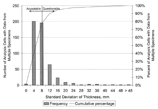
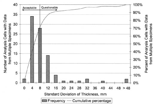
Code Description 51 Intact core; excellent condition; suitable for testing
52 Hairline cracks on the surface of the core; suitable for testing
53 Cracks or voids visible along the side of the core; suitable for testing
54 Badly cracked or damaged core; unsuitable for testing
55 Ridges on the sides of the cores (identified by placing a straight edge along the side of the core when the distance between the straight edge and core face is 1.6 mm or greater); such a condition should be recorded if the core is used for any other test
56 Very rough and uneven bottom surface of the core (identified with this code when less than75 percent of the surface area is in contact with a level surface when the core is perpendicular to the surface)
57 Core extremely damaged from sampling, shipping, or laboratory handling; unsuitable for testing
58 Core was sawed in the laboratory to remove the core from the underlying bonded layer ofbase, subbase, or AC
59 Core consisted of two or more PCC layers; core was sawed in the laboratory and appropriate layer numbers were assigned to each PCC layer
60 One or more PCC layers have become separated; appropriate layer numbers were assigned toeach PCC layer
61 Segregation of coarse and fine aggregate is observed over 25 percent or more of the surface area of the core
62 Voids in the matrix of the PCC mixture are observed along the sides of the core
63 Voids due to loss of coarse and fine aggregate are observed along the sides of the core
64 Core is missing significant portions and cannot be considered a coherent cylindrical core;unsuitable for testing
65 Coarse aggregate along the face of the core contains 50 percent or more of crushed materials with fractured faces
66 Coarse aggregate along the face of the core is a mixture of uncrushed gravel and crushedgravel or stone
67 The exposed aggregates along the face of the core are lightweight aggregate
68 More than 10 percent of the surface area of the core contains soft and deleterious aggregateparticles or clay balls (soft aggregates are defined as those aggregates that can be easilyscratched with a knife)
69 Cracks are generally across or through the coarse aggregate
70 Cracks are generally around the periphery of the coarse aggregate
71 Cracks are associated with embedded steel
72 Rims are observed on aggregate
73 Fine aggregate is natural sand
74 Fine aggregate is manufactured sand
75 Fine aggregate is a mixture of natural and manufactured sand
76 Steel is present in the core (give type size and location of steel in a separate note)
77 Steel is corroded
78 Core indicates D-cracking (a series of closely spaced crescent-shaped hairline cracks that appear at a PCC pavement surface at longitudinal joints/cracks and transverse joints/cracks)
79 Core indicates deterioration due to freeze-thaw cycles
80 Core indicates sulfate attack
81 Core indicates alkali silica reactivity (expansion of reactive aggregates)
82 Skewed core (when either end of the core departs from perpendicularity to the axis by more than 0.5 degrees or 3 mm in 300 mm, as tested by placing the core on a level surface)
99 Other comment (describe in a note)
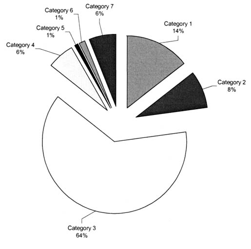
Expt. Type Layer Type Test Type LTPP Designation LTPP Protocol Min. No. of Tests per Layer Designated Sampling Locations GPS-3, 4, 5, and 9 PCC Comp. strength PC01 P61 2 C2 C8
GPS-7 PCC Comp. strength PC01 P61 2 C8 C20
SPS-2 PCC Comp. strength
(14 day, 3.8 MPa)PC01 P61 3 (cylinder) B21-B23
SPS-2 PCC Comp. strength
(14 day, 3.8 MPa)PC01 P61 6 (core) C1 C10 C18 C26 C34 C43
SPS-2 PCC Comp. strength
(14 day, 6.2 MPa)PC01 P61 3 (cylinder) B24-B26
SPS-2 PCC Comp. strength
(14 day, 6.2 MPa)PC01 P61 6 (core) C51 C59 C67 C75 C83 C91
SPS-2 PCC Comp. strength
(28 day, 3.8 MPa)PC01 P61 3 (cylinder) B21-B23
SPS-2 PCC Comp. strength
(28 day, 3.8 MPa)PC01 P61 6 (core) C2 C11 C19 C27 C35 C44
SPS-2 PCC Comp. strength
(28 day, 6.2 MPa)PC01 P61 3 (cylinder) B24-B26
SPS-2 PCC Comp. strength
(28 day, 6.2 MPa)PC01 P61 6 (core) C52 C60 C68 C76 C84 C92
SPS-2 PCC Comp. strength
(1 year, 3.8 MPa)PC01 P61 3 (cylinder) B21-B23
SPS-2 PCC Comp. strength
(1 year, 3.8 MPa)PC01 P61 6 (core) C3 C12 C20 C28 C36 C45
SPS-2 PCC Comp. strength
(1 year, 6.2 MPa)PC01 P61 3 (cylinder) B24-B26
SPS-2 PCC Comp. strength
(1 year, 6.2 MPa)PC01 P61 6 (core) C53 C61 C69 C77 C85 C93
SPS-2 LCB 7 day PC01 P61 6 (cylinder) B19 B20
SPS-2 LCB 14 day PC01 P61 8 (core) C18 C22 C26 C30 C67 C70 C75 C79
SPS-2 LCB 28 day PC01 P61 6 (cylinder) B19 B20
SPS-2 LCB 28 day PC01 P61 8 (core) C19 C23 C27 C31 C68 C71 C76 C80
SPS-2 LCB 1 year PC01 P61 6 (cylinder) B19 B20
SPS-2 LCB 1 year PC01 P61 8 (core) C20 C24 C28 C32 C69 C72 C77 C81
SPS-6 PCC
(cores)Comp. strength PC01 P61 10 C1 C3 C5 C7 C9 C11 C13 C15 C17 C19
SPS-7 PCC--Overlay
(Postconstruction cores)Comp. strength 14 day PC01 P61 4 C12 C15 C17 C19
SPS-7 PCC--Overlay
(Postconstruction cores)Comp. strength 28 day PC01 P61 4 C43 C50 C57 C64
SPS-7 PCC--Overlay
(Postconstruction cores)Comp. strength 365 day PC01 P61 4 C86 C93 C100 C107
SPS-7 PCC--Overlay
(During construction cylinders)Comp. strength 14 day PC01 P61 6 FC1 FC2 FC3 (75-mm cores)
SPS-7 PCC--Overlay
(During construction cylinders)Comp. strength 14 day PC01 P61 6 FC4 FC5 FC6 (125-mm cores)
SPS-7 PCC--Overlay
(During construction cylinders)Comp. strength 14 day PC01 P61 6 FC1 FC2 FC3 (75-mm cores)
SPS-7 PCC--Overlay
(During construction cylinders)Comp. strength 28 day PC01 P61 6 FC4 FC5 FC6 (125-mm cores)
SPS-7 PCC--Overlay
(During construction cylinders)Comp. strength 365 day PC01 P61 6 FC1 FC2 FC3 (75-mm cores)
SPS-7 PCC--Overlay
(During construction cylinders)Comp. strength 365 day PC01 P61 6 FC4 FC5 FC6 (125-mm cores)
SPS-7 PCC--Original layer
(cores)Comp. strength PC01 P61 9 C21 C25 C29 C33 C37 C44 C51 C58
SPS-8 PCC
("as-delivered" cylinders)Comp. strength 14 day PC01 P61 3 FC1 FC2 FC3
SPS-8 PCC
("as-delivered" cylinders)Comp. strength 28 day PC01 P61 3 FC1 FC2 FC3
SPS-8 PCC
("as-delivered" cylinders)Comp. strength 365 day PC01 P61 3 FC1 FC2 FC3
SPS-8 PCC
("as-placed" cores)Comp. strength 14 day PC01 P61 3 C1 C10 C20
SPS-8 PCC
("as-placed" cores)Comp. strength 28 day PC01 P61 3 C2 C11 C21
SPS-8 PCC
("as-placed" cores)Comp. strength 365 day PC01 P61 3 C4 C13 C22
Expt. Type Expt. No. Total No. of Records at Levels A to E Total No. of Records at Level E No. of Usable Records at Level E Percent Usable Records at Level E Total No. of Analysis Cells Represented at Level E GPS 3 226 225 225 100 113
GPS 4 120 117 117 98 59
GPS 5 158 157 157 99 79
GPS 7A 65 64 64 98 33
GPS 7B 18 15 131 72 7
GPS 9 94 94 892 95 45
SPS 1 21 0 0 0 N/A
SPS 2 1334 1091 10083 76 75--PCC
44--LCBSPS 6 96 71 624 65 9
SPS 7 236 182 1785 75 3--Original
12--OverlaySPS 8 24 23 23 96 9
Unclassified6 N/A 4 4 N/A N/A N/A
2Three records with suspicious layer numbering; two records with no corresponding TST_L05B information required to verify layer type.
3Eighteen records with wrong material type assignment; four records with no compressive strength data; 61 records with no TST_L05B information.
4Nine records with no compressive strength data.
5Four records with no compressive strength data.
6These records could not be identified with any LTPP experiment.
Key Fields GPS Experiments (all) SPS-2 SPS-6 SPS-7 SPS-8 Experiment type X X X X X
Experiment number X X X X X
SHRP_ID X -- -- -- --
State code X X X X X
Layer number X -- X X X
Material code X X X X X
Construction number X X X X X
Target strength -- X -- -- --
Specimen type -- X -- X X
Specimen age -- X -- X X
Experiment Type Total Number of Analysis Cells Represented at Level E Number with Less than Minimum Samples Percent Layers with Less than Minimum Samples GPS-3 113 1 1
GPS-4 59 1 2
GPS-5 79 1 4
GPS-7A 33 2 6
GPS-7B 7 1 14
GPS-9 45 1 2
State Code Specimen Type Specimen Age Min. Samples Required Samples Tested Sampling Plan Satisfied? 4 Core 7 days --1 6 N/A
4 Core 28 days 8 6 No
4 Core 365 days 8 6 No
4 Cylinder 7 days 6 6 Yes
4 Cylinder 28 days 6 5 No
4 Cylinder 365 days 6 2 No
10 Core 14 days 8 9 Yes
10 Core 28 days 8 0 No
10 Core 365 days 8 11 Yes
10 Cylinder 7 days 6 0 No
10 Cylinder 14 days --1 2 N/A
10 Cylinder 28 days 6 2 No
10 Cylinder 365 days 6 2 No
19 Core 7 days --1 8 N/A
19 Core 28 days 8 3 No
19 Core 365 days 8 8 Yes
19 Cylinder 7 days 6 3 No
19 Cylinder 28 days 6 3 No
19 Cylinder 365 days 6 3 No
20 Core 14 days 8 0 No
20 Core 28 days 8 0 No
20 Core 365 days 8 0 No
20 Cylinder 7 days 6 3 No
20 Cylinder 14 days --1 3 N/A
20 Cylinder 28 days 6 7 Yes
20 Cylinder 365 days 6 6 Yes
26 Core 14 days 8 0 No
26 Core 28 days 8 0 No
26 Core 365 days 8 7 No
26 Cylinder 7 days 6 9 Yes
26 Cylinder 28 days 6 9 Yes
26 Cylinder 365 days 6 8 Yes
32 Core 14 days 8 8 Yes
32 Core 28 days 8 8 Yes
32 Core 365 days 8 8 Yes
32 Cylinder 7 days 6 7 Yes
32 Cylinder 28 days 6 8 Yes
32 Cylinder 365 days 6 8 Yes
38 Core 14 days 8 0 No
38 Core 28 days 8 1 No
38 Core 365 days 8 4 No
38 Cylinder 7 days 6 0 No
38 Cylinder 28 days 6 0 No
38 Cylinder 365 days 6 0 No
39 Core 7 days --1 4 N/A
39 Core 14 days 8 0 No
39 Core 28 days 8 8 Yes
39 Core 365 days 8 8 Yes
39 Cylinder 7 days 6 3 No
39 Cylinder 28 days 6 6 Yes
39 Cylinder 365 days 6 6 Yes
53 Core 14 days 8 8 Yes
53 Core 28 days 8 8 Yes
53 Core 365 days 8 8 Yes
53 Cylinder 7 days 6 8 Yes
53 Cylinder 28 days 6 8 Yes
53 Cylinder 365 days 6 7 Yes
State Code Target Strength, MPa Specimen Type Specimen Age Min. Samples Required Samples Tested Sampling Plan Satisfied? 4 3.8 Core 14 days 6 10 Yes
4 3.8 Core 28 days 6 9 Yes
4 3.8 Core 365 days 6 9 Yes
4 3.8 Cylinder 14 days 3 0 No
4 3.8 Cylinder 28 days 3 0 No
4 3.8 Cylinder 365 days 3 0 No
4 6.2 Core 14 days 6 8 Yes
4 6.2 Core 28 days 6 8 Yes
4 6.2 Core 365 days 6 9 Yes
4 6.2 Cylinder 14 days 3 0 No
4 6.2 Cylinder 28 days 3 0 No
4 6.2 Cylinder 365 days 3 0 No
5 3.8 Core 14 days 6 0 No
5 3.8 Core 28 days 6 0 No
5 3.8 Core 365 days 6 19 Yes
5 3.8 Cylinder 14 days 3 0 No
5 3.8 Cylinder 28 days 3 0 No
5 3.8 Cylinder 365 days 3 11 No
5 6.2 Core 14 days 6 0 No
5 6.2 Core 28 days 6 0 No
5 6.2 Core 365 days 6 18 Yes
5 6.2 Cylinder 14 days 3 0 No
5 6.2 Cylinder 28 days 3 0 No
5 6.2 Cylinder 365 days 3 0 No
8 3.8 Core 14 days 6 18 Yes
8 3.8 Core 28 days 6 16 Yes
8 3.8 Core 365 days 6 20 Yes
8 3.8 Cylinder 14 days 3 0 No
8 3.8 Cylinder 28 days 3 0 No
8 3.8 Cylinder 365 days 3 0 No
8 6.2 Core 14 days 6 15 Yes
8 6.2 Core 28 days 6 18 Yes
8 6.2 Core 365 days 6 20 Yes
8 6.2 Cylinder 14 days 3 0 No
8 6.2 Cylinder 28 days 3 6 Yes
8 6.2 Cylinder 365 days 3 6 Yes
10 3.8 Core 14 days 6 13 Yes
10 3.8 Core 28 days 6 6 Yes
10 3.8 Core 365 days 6 9 Yes
10 3.8 Cylinder 14 days 3 0 No
10 3.8 Cylinder 28 days 3 0 No
10 3.8 Cylinder 365 days 3 0 No
10 6.2 Core 14 days 6 7 Yes
10 6.2 Core 28 days 6 5 No
10 6.2 Core 365 days 6 7 Yes
10 6.2 Cylinder 14 days 3 0 No
10 6.2 Cylinder 28 days 3 0 No
10 6.2 Cylinder 365 days 3 0 No
19 3.8 Core 14 days 6 7 Yes
19 3.8 Core 28 days 6 8 Yes
19 3.8 Core 365 days 6 6 Yes
19 3.8 Cylinder 14 days 3 0 No
19 3.8 Cylinder 28 days 3 0 No
19 3.8 Cylinder 365 days 3 0 No
19 6.2 Core 14 days 6 7 Yes
19 6.2 Core 28 days 6 8 Yes
19 6.2 Core 365 days 6 9 Yes
19 6.2 Cylinder 14 days 3 0 No
19 6.2 Cylinder 28 days 3 0 No
19 6.2 Cylinder 365 days 3 0 No
20 3.8 Core 14 days 6 8 Yes
20 3.8 Core 28 days 6 7 Yes
20 3.8 Core 365 days 6 7 Yes
20 3.8 Cylinder 14 days 3 0 No
20 3.8 Cylinder 28 days 3 0 No
20 3.8 Cylinder 365 days 3 0 No
20 6.2 Core 14 days 6 4 No
20 6.2 Core 28 days 6 5 No
20 6.2 Core 365 days 6 3 No
20 6.2 Cylinder 14 days 3 0 No
20 6.2 Cylinder 28 days 3 0 No
20 6.2 Cylinder 365 days 3 0 No
26 3.8 Core 14 days 6 8 Yes
26 3.8 Core 28 days 6 6 Yes
26 3.8 Core 365 days 6 9 Yes
26 3.8 Cylinder 14 days 3 0 No
26 3.8 Cylinder 28 days 3 0 No
26 3.8 Cylinder 365 days 3 0 No
26 6.2 Core 14 days 6 4 No
26 6.2 Core 28 days 6 6 Yes
26 6.2 Core 365 days 6 7 Yes
26 6.2 Cylinder 14 days 3 0 No
26 6.2 Cylinder 28 days 3 0 No
26 6.2 Cylinder 365 days 3 0 No
32 3.8 Core 14 days 6 9 Yes
32 3.8 Core 28 days 6 10 Yes
32 3.8 Core 365 days 6 10 Yes
32 3.8 Cylinder 14 days 3 0 No
32 3.8 Cylinder 28 days 3 0 No
32 3.8 Cylinder 365 days 3 0 No
32 6.2 Core 14 days 6 8 Yes
32 6.2 Core 28 days 6 7 Yes
32 6.2 Core 365 days 6 7 Yes
32 6.2 Cylinder 14 days 3 0 No
32 6.2 Cylinder 28 days 3 0 No
32 6.2 Cylinder 365 days 3 0 No
37 3.8 Core 14 days 6 3 No
37 3.8 Core 28 days 6 3 No
37 3.8 Core 365 days 6 2 No
37 3.8 Cylinder 14 days 3 0 No
37 3.8 Cylinder 28 days 3 11 No
37 3.8 Cylinder 365 days 3 0 No
37 6.2 Core 14 days 6 2 No
37 6.2 Core 28 days 6 3 No
37 6.2 Core 365 days 6 4 No
37 6.2 Cylinder 14 days 3 4 Yes
37 6.2 Cylinder 28 days 3 4 Yes
37 6.2 Cylinder 365 days 3 2 No
38 3.8 Core 14 days 6 5 No
38 3.8 Core 28 days 6 3 No
38 3.8 Core 365 days 6 15 Yes
38 3.8 Cylinder 14 days 3 0 No
38 3.8 Cylinder 28 days 3 0 No
38 3.8 Cylinder 365 days 3 0 No
38 6.2 Core 14 days 6 4 No
38 6.2 Core 28 days 6 11 No
38 6.2 Core 365 days 6 16 Yes
38 6.2 Cylinder 14 days 3 0 No
38 6.2 Cylinder 28 days 3 0 No
38 6.2 Cylinder 365 days 3 0 No
39 3.8 Core 14 days 6 9 Yes
39 3.8 Core 28 days 6 11 Yes
39 3.8 Core 365 days 6 7 Yes
39 3.8 Cylinder 14 days 3 0 No
39 3.8 Cylinder 28 days 3 0 No
39 3.8 Cylinder 365 days 3 0 No
39 6.2 Core 14 days 6 7 Yes
39 6.2 Core 28 days 6 5 No
39 6.2 Core 365 days 6 4 No
39 6.2 Cylinder 14 days 3 0 No
39 6.2 Cylinder 28 days 3 0 No
39 6.2 Cylinder 365 days 3 0 No
53 3.8 Core 14 days 6 12 Yes
53 3.8 Core 28 days 6 12 Yes
53 3.8 Core 365 days 6 11 Yes
53 3.8 Cylinder 14 days 3 0 No
53 3.8 Cylinder 28 days 3 0 No
53 3.8 Cylinder 365 days 3 0 No
53 6.2 Core 14 days 6 6 Yes
53 6.2 Core 28 days 6 6 Yes
53 6.2 Core 365 days 6 7 Yes
53 6.2 Cylinder 14 days 3 0 No
53 6.2 Cylinder 28 days 3 0 No
53 6.2 Cylinder 365 days 3 0 No
State Code Min. Samples Required Samples Tested Sampling Plan Satisfied? 4 10 9 No
17 10 8 No
26 10 18 Yes
29 10 11 Yes
40 10 10 Yes
42 10 6 No
State Code Layer Type Specimen Type Specimen Age Min. Samples Required Samples Tested Sampling Plan Satisfied? 19 Existing PCC Core N/A 9 6 No
19 PCC Overlay
(during construction)Cylinder 14 days 6 0 No
19 PCC Overlay
(during construction)Cylinder 28 days 6 0 No
19 PCC Overlay
(during construction)Cylinder 365 days 6 0 No
19 PCC Overlay
(postconstruction)Core 14 days 4 3 No
19 PCC Overlay
(postconstruction)Core 28 days 4 3 No
19 PCC Overlay
(postconstruction)Core 365 days 4 4 Yes
22 Existing PCC Core N/A 9 7 No
22 PCC Overlay
(during construction)Cylinder 14 days 6 4 No
22 PCC Overlay
(during construction)Cylinder 28 days 6 8 Yes
22 PCC Overlay
(during construction)Cylinder 365 days 6 0 No
22 PCC Overlay
(postconstruction)Core 14 days 4 4 Yes
22 PCC Overlay
(postconstruction)Core 28 days 4 4 Yes
22 PCC Overlay
(postconstruction)Core 365 days 4 4 Yes
27 Existing PCC Core N/A 9 0 No
27 PCC Overlay
(during construction)Cylinder 14 days 6 0 No
27 PCC Overlay
(during construction)Cylinder 28 days 6 0 No
27 PCC Overlay
(during construction)Cylinder 365 days 6 0 No
27 PCC Overlay
(postconstruction)Core 14 days 4 0 No
27 PCC Overlay
(postconstruction)Core 28 days 4 0 No
27 PCC Overlay
(postconstruction)Core 365 days 4 3 No
29 Existing PCC Core N/A 9 22 Yes
29 PCC Overlay
(during construction)Cylinder 14 days 6 2 Yes
29 PCC Overlay
(during construction)Cylinder 28 days 6 28 Yes
29 PCC Overlay
(during construction)Cylinder 365 days 6 0 No
29 PCC Overlay
(post construction)Core 14 days 4 0 No
29 PCC Overlay
(post construction)Core 28 days 4 0 No
29 PCC Overlay
(post construction)Core 365 days 4 4 Yes
State Code Layer Type Specimen Type Specimen Age Min. Samples Required Samples Tested Sampling Plan Satisfied? 8 PCC Overlay (during construction) Cylinder 14 days 3 3 Yes
8 PCC Overlay (during construction) Cylinder 28 days 3 3 Yes
8 PCC Overlay (during construction) Cylinder 365 days 3 0 No
8 PCC Overlay (postconstruction) Core 14 days 3 3 Yes
8 PCC Overlay (postconstruction) Core 28 days 3 3 Yes
8 PCC Overlay (postconstruction) Core 365 days 3 0 No
39 PCC Overlay (during construction) Cylinder 14 days 3 3 Yes
39 PCC Overlay (during construction) Cylinder 28 days 3 3 Yes
39 PCC Overlay (during construction) Cylinder 365 days 3 0 No
39 PCC Overlay (postconstruction) Core 14 days 3 2 No
39 PCC Overlay (postconstruction) Core 28 days 3 3 Yes
39 PCC Overlay (postconstruction) Core 365 days 3 0 No
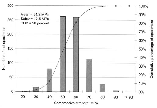
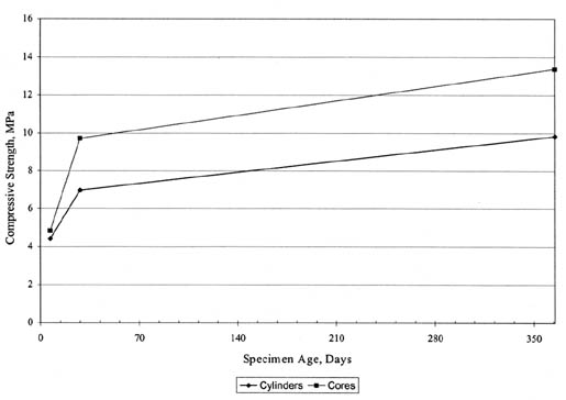
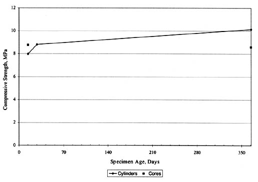
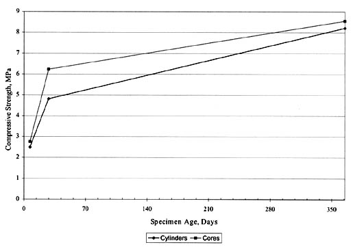
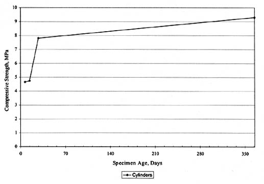
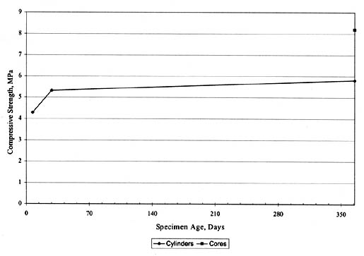
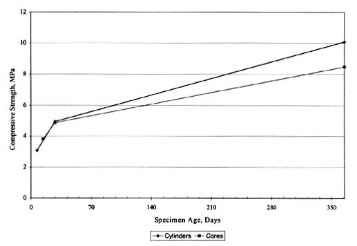
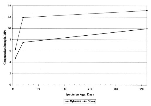
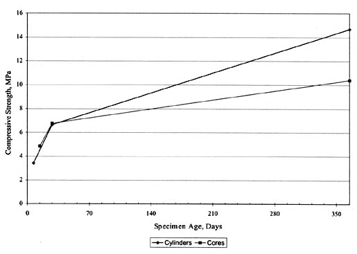
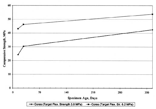
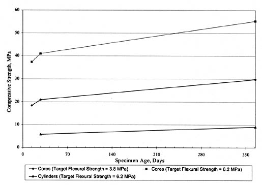
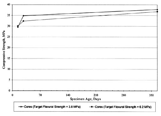
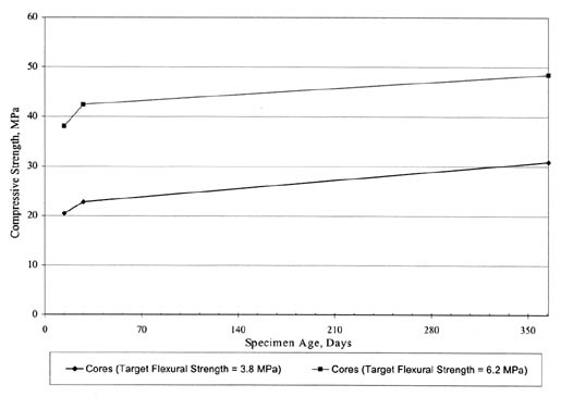
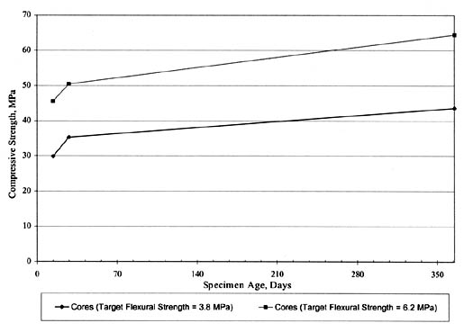
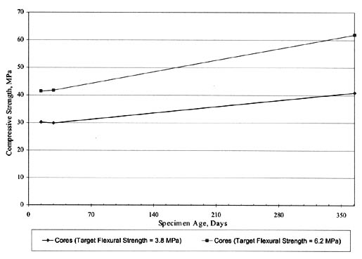
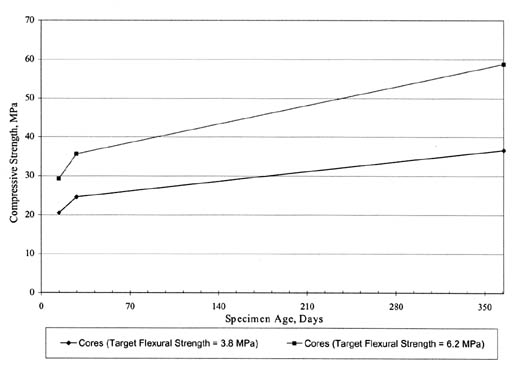
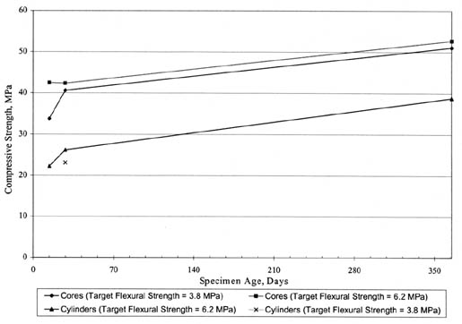
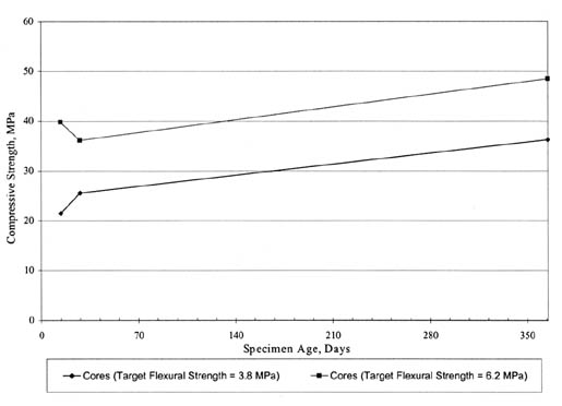
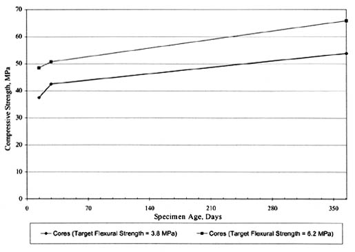
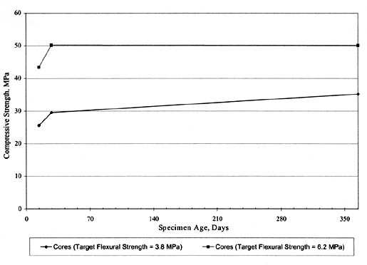
Reference Specimen Type COV, percent Standard Deviation Bartlett et al., 1995(33) 28-day Core 12 to 13 --
Hughes, 1996(13) 28-day Core 17 --
Demos et al., 1995 28-day Cylinders 12.9 --
Darter, 1972(27) 28-day Specimens 9.8 to 16.5 --
Di Cocco, 1973(36) 28-day Cylinders -- 4.98 MPa
Neaman et al., 1967(29) 28-day Cylinder 18.95 --
ACPA, 1995(37) 28-day Specimens Ready mix 7 to 13
Central mix 5 to 12--
McMahon et al., 1990(30) 28-day Specimen -- 3.2 to 4.57 MPa
Steele et al., 1966(38) 28-day Cylinders 8 to 15 --
Hughes et al., 1998(31) 28-day Cores
28-day Cylinders13.410.4 --
Age at Test Strength Ratio for Moist Curing1 Strength Ratio for Outdoor Exposure1 1 day 0.18 3 days 0.46 0.53
7 days 0.70 0.78
28 days 1.00 1
3 months 1.14 1.09
1 year 1.22 1.19
5 years 1.33 1.37
10 years 1.33 1.39
20+ years 1.44 1.42
Experiment Type Layer Type Test Type LTPP Designation LTPP Protocol Min No. of Tests per Layer Designated Sampling Location GPS 1-7 and 9 PCC CTE PC03 P63 -- --
SPS-2 PCC CTE PC03 P63 2 C42, C99
SPS-6 PCC CTE PC03 P63 3 A1 A2 A3
SPS-7 PCC overlay
(postconstruction)CTE
(14 day)PC03 P63 1 C11
SPS-7 PCC overlay
(preconstruction)CTE PC03 P63 1 C11
SPS-8 PCC CTE PC03 P63 1 C18
Expt.Type Expt. No. Total No. of Records at All Levels Total No. of Records at Level E No. of Usable Records at Level E Percent Usable Records at Level E Total No. of Analysis Cells Represented GPS 3 67 67 67 100 67
GPS 4 48 48 48 100 48
GPS 5 54 54 54 100 54
GPS 7B 4 4 4 100 4
Experiment Type Experiment Number Total Number of Specimens at All Levels Total Number of Specimens at Level E Percentage of Specimens at Level E Total Number of PCC Layers Represented1 SPS 1 12 0 0 --
SPS 2 282 274 97 23
SPS 2S2 80 0 0 --
SPS 7 36 28 77 3
SPS 7S2 6 0 0 --
SPS 8 11 10 91 2
1SPS-2 experiments sections with different target strengths and SPS-7 sections with different target thicknesses were considered as different layers. SPS-2 and SPS-7 sections, therefore, had two PCC layers per experiment, whereas SPS-8 experiments had one. The total number of analysis cells represented by these layers was 90.
2Supplementary test sections.
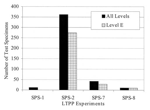
Experiment Type Layer Material Type Target Age, days Target Compressive Strength, MPa Target Thickness, mm LTPP Designation SHRP Test Protocol Minimum Number of Tests Minimum Number of Tests per Cell Sampling Location1 SPS-2 PCC 14 3.8 -- PC09 P69 3 3 B21-B23
SPS-2 PCC 28 3.8 -- PC09 P69 3 3 B21-B23
SPS-2 PCC 365 3.8 -- PC09 P69 3 3 B21-B23
SPS-2 PCC 14 6.2 -- PC09 P69 3 3 B24-B26
SPS-2 PCC 28 6.2 -- PC09 P69 3 3 B24-B26
SPS-2 PCC 365 6.2 -- PC09 P69 3 3 B24-B26
SPS-7 PCC 14 -- 75 PC09 P69 3 3 FC1 FC2 FC3
SPS-7 PCC 28 -- 75 PC09 P69 3 3 FC1 FC2 FC3
SPS-7 PCC 365 -- 75 PC09 P69 3 3 FC1 FC2 FC3
SPS-7 PCC 14 -- 125 PC09 P69 3 3 FC4 FC5 FC6
SPS-7 PCC 28 -- 125 PC09 P69 3 3 FC4 FC5 FC6
SPS-7 PCC 365 -- 125 PC09 P69 3 3 FC4 FC5 FC6
SPS-8 PCC 14 -- -- PC09 P69 3 3 FC1 FC2 FC3
SPS-8 PCC 28 -- -- PC09 P69 3 3 FC1 FC2 FC3
SPS-8 PCC 365 -- -- PC09 P69 3 3 FC1 FC2 FC3
State Code SPS Experiment Type SPS-2 Target Strength, MPa SPS-7 Target Thickness, mm Specimen Age, days Number of Specimens Tested Target Minimum Minimum Satisfied? 4 SPS-2 3.8 -- 14 3 3 Yes
4 SPS-2 3.8 -- 28 3 3 Yes
4 SPS-2 3.8 -- 365 3 3 Yes
4 SPS-2 6.2 -- 14 6 3 Yes
4 SPS-2 6.2 -- 28 6 3 Yes
4 SPS-2 6.2 -- 365 6 3 Yes
5 SPS-2 3.8 -- 14 5 3 Yes
5 SPS-2 3.8 -- 28 5 3 Yes
5 SPS-2 3.8 -- 365 5 3 Yes
5 SPS-2 6.2 -- 14 2 3 No
5 SPS-2 6.2 -- 28 2 3 No
5 SPS-2 6.2 -- 365 2 3 No
8 SPS-2 3.8 -- 14 9 3 Yes
8 SPS-2 3.8 -- 28 9 3 Yes
8 SPS-2 3.8 -- 365 7 3 Yes
8 SPS-2 6.2 -- 14 9 3 Yes
8 SPS-2 6.2 -- 28 9 3 Yes
8 SPS-2 6.2 -- 365 9 3 Yes
10 SPS-2 3.8 -- 14 3 3 Yes
10 SPS-2 3.8 -- 28 3 3 Yes
10 SPS-2 3.8 -- 365 3 3 Yes
10 SPS-2 6.2 -- 14 3 3 Yes
10 SPS-2 6.2 -- 28 2 3 No
10 SPS-2 6.2 -- 365 2 3 No
19 SPS-2 3.8 -- 14 3 3 Yes
19 SPS-2 3.8 -- 28 3 3 Yes
19 SPS-2 3.8 -- 365 3 3 Yes
19 SPS-2 6.2 -- 14 3 3 Yes
19 SPS-2 6.2 -- 28 3 3 Yes
19 SPS-2 6.2 -- 365 3 3 Yes
20 SPS-2 3.8 -- 14 7 3 Yes
20 SPS-2 3.8 -- 28 7 3 Yes
20 SPS-2 3.8 -- 365 7 3 Yes
20 SPS-2 6.2 -- 14 6 3 Yes
20 SPS-2 6.2 -- 28 5 3 Yes
20 SPS-2 6.2 -- 365 4 3 Yes
26 SPS-2 3.8 -- 14 0 3 No
26 SPS-2 3.8 -- 28 0 3 No
26 SPS-2 3.8 -- 365 3 3 Yes
26 SPS-2 6.2 -- 14 0 3 No
26 SPS-2 6.2 -- 28 0 3 No
26 SPS-2 6.2 -- 365 3 3 Yes
32 SPS-2 3.8 -- 14 3 3 Yes
32 SPS-2 3.8 -- 28 3 3 Yes
32 SPS-2 3.8 -- 365 3 3 Yes
32 SPS-2 6.2 -- 14 3 3 Yes
32 SPS-2 6.2 -- 28 3 3 Yes
32 SPS-2 6.2 -- 365 3 3 Yes
37 SPS-2 3.8 -- 14 0 3 No
37 SPS-2 3.8 -- 28 0 3 No
37 SPS-2 3.8 -- 365 2 3 No
37 SPS-2 6.2 -- 14 0 3 No
37 SPS-2 6.2 -- 28 0 3 No
37 SPS-2 6.2 -- 365 0 3 No
39 SPS-2 3.8 -- 14 3 3 Yes
39 SPS-2 3.8 -- 28 3 3 Yes
39 SPS-2 3.8 -- 365 3 3 Yes
39 SPS-2 6.2 -- 14 3 3 Yes
39 SPS-2 6.2 -- 28 3 3 Yes
39 SPS-2 6.2 -- 365 3 3 Yes
53 SPS-2 3.8 -- 14 4 3 Yes
53 SPS-2 3.8 -- 28 4 3 Yes
53 SPS-2 3.8 -- 365 4 3 Yes
53 SPS-2 6.2 -- 14 3 3 Yes
53 SPS-2 6.2 -- 28 3 3 Yes
53 SPS-2 6.2 -- 365 3 3 Yes
55 SPS-2 3.8 -- 14 3 3 Yes
55 SPS-2 3.8 -- 28 3 3 Yes
55 SPS-2 3.8 -- 365 0 3 No
55 SPS-2 6.2 -- 14 4 3 Yes
55 SPS-2 6.2 -- 28 2 3 No
55 SPS-2 6.2 -- 365 0 3 No
22 SPS-7 -- 75 14 4 3 Yes
22 SPS-7 -- 75 28 2 3 No
22 SPS-7 -- 75 365 0 3 No
22 SPS-7 -- 125 14 3 3 Yes
22 SPS-7 -- 125 28 3 3 Yes
22 SPS-7 -- 125 365 0 3 No
29 SPS-7 -- 75 14 0 3 No
29 SPS-7 -- 75 28 8 3 Yes
29 SPS-7 -- 75 365 0 3 No
29 SPS-7 -- 125 14 0 3 No
29 SPS-7 -- 125 28 8 3 Yes
29 SPS-7 -- 125 365 0 3 No
8 SPS-8 -- -- 14 3 3 Yes
8 SPS-8 -- -- 28 3 3 Yes
8 SPS-8 -- -- 365 0 3 No
39 SPS-8 -- -- 14 3 3 Yes
39 SPS-8 -- -- 28 1 3 No
39 SPS-8 -- -- 365 0 3 No
The coefficient of variation of test results has been observed to be dependent on the strength levels of the beams. The single operator coefficient of variability has been found to be 5.7 percent. The multilaboratory coefficient of variability has been found to be 7.0 percent.
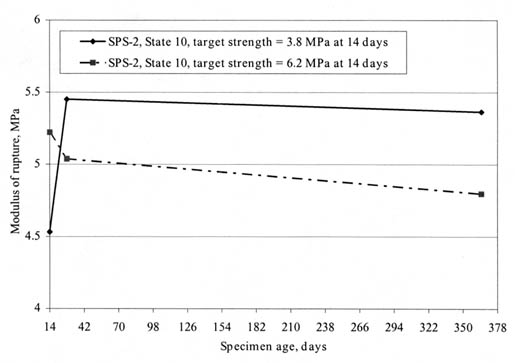
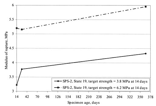
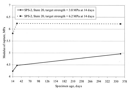
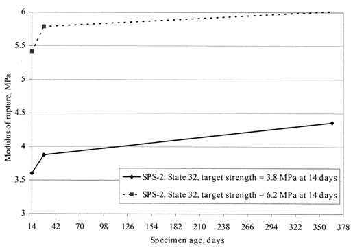
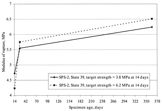
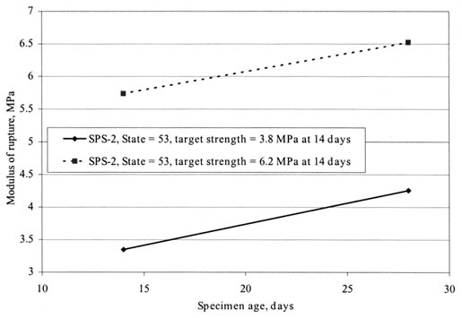
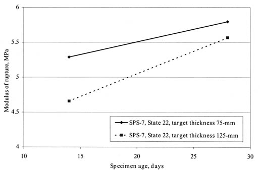
Data Element Reference Coefficient of Variation, percent Flexural Strength Demos et al.(35) 8.1
Flexural Strength Darter(27) 7.6 to 9.7
Flexural Strength Hughes et al. 1998(31) 10.4 to 12.7
Flexural Strength Indiana Contractors QC(31) 5
Flexural Strength Lytton and Zollinger(32) 8 to 10
Flexural Strength Indiana DOT QC(31) 5.8
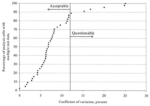
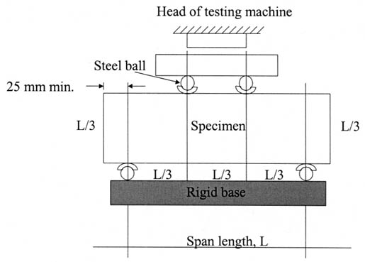
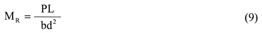
MR = flexural strength
P = maximum load applied, MPa
L = specimen span length
b = specimen width
d = specimen depth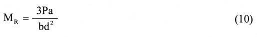
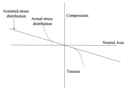
![]()
STRRATIO = ratio of MR at a given age to MR at 28 days
AGE = specimen age in years
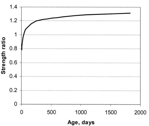
Specimen Age, days Strength Ratio 14 0.91
28 1.00
365 1.26
Model Source MR = 0.62 (sigmac)0.5 (stress in MPa) Price (American Concrete Institute, [ACI])(42)
MR = k2(sigmac)k1(k2 ranges from 3 to 6, k1 from 0.3 to 0.8, stress in psi) Neville(43)
MR = 8.3 (sigmac)0.5 (stress in psi) Teychenne(44)
MR = 8.3 / (4 + 12000/sigmac) (stress in psi) Sozen(45)
MR = 9.5 (sigmac)0.5 (stress in psi) Comite Europeen du Beton(43)
Experiment Type Layer Type Test Type LTPP Designation LTPP Protocol Minimum Number of Tests per Layer Designated Sampling Location1 GPS 2, 6 and 7 Treated base/subbase and subgrade Unconfined compressive strength TB02 P32 2 C10 and C22 or one from (C7, C8, C9) and (C19, C20, C21)
GPS 3, 4, 5 and 9 Treated base/subbase and subgrade Unconfined compressive strength TB02 P32 2 C4 and C10 or one from (C1, C2, C3) and (C7, C8, C9)
SPS 5 Treated base/subbase and subgrade Unconfined compressive strength TB02 P32 3 [C4-C5] [C15 C16] [C23 C24]
SPS 6 Treated base/subbase and subgrade Unconfined compressive strength TB02 P32 3 C5 C11 C19
SPS 7 Treated base/subbase and subgrade Unconfined compressive strength TB02 P32 3 C1 C4 C7
Expt. Type Expt. No. No. of Records at Levels A to E No. of Records at Level E No. of Usable Records at Level E Percent Usable Records at Level E Total Number of Analysis Cells Represented GPS 2 70 68 68 97 34
GPS 3 66 66 651 98 34
GPS 4 13 11 11 85 7
GPS 5 32 32 32 100 17
GPS 6B 7 7 7 100 4
GPS 7A 6 6 6 100 3
GPS 9 6 6 6 100 3
SPS 2 7 7 02 0 N/A
SPS 5 2 2 03 0 N/A
SPS 6 5 5 5 100 2
2Seven records belong to the TST_PC01 table.
3Two records belong to supplemental sections.
Key Fields GPS Experiments (All) SPS Experiments (All) Experiment type X X
Experiment number X X
SHRP_ID X --
SPS cell identification number -- X
State code X X
Layer number X --
Material code X X
Construction number X X
Experiment Type No. of Analysis Cells with Data at Level E No. with Less than Minimum Required Samples Percent Cells with Less than Min. Required Samples GPS-2 34 0 0
GPS-3 34 3 9
GPS-4 7 3 43
GPS-5 17 2 12
GPS-6B 4 1 25
GPS-7A 3 0 0
GPS-9 3 0 0
SPS-6 2 1 50
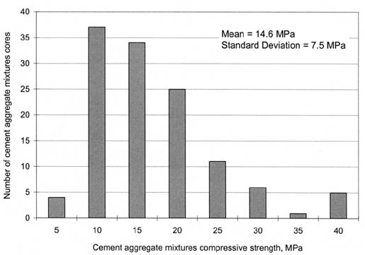
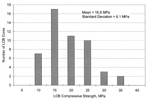
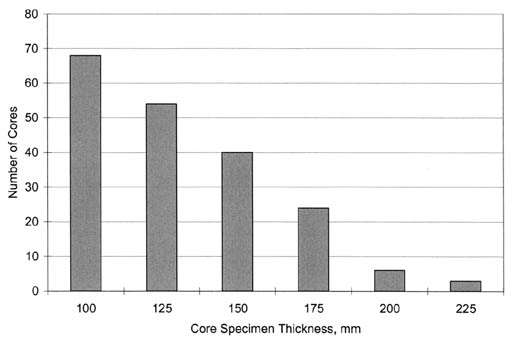
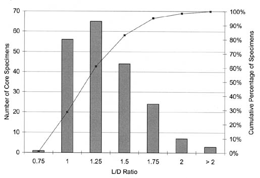
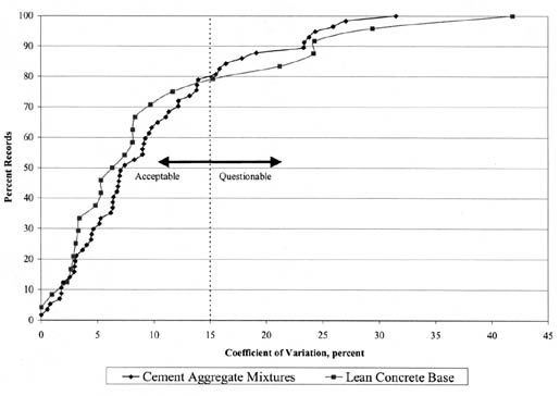
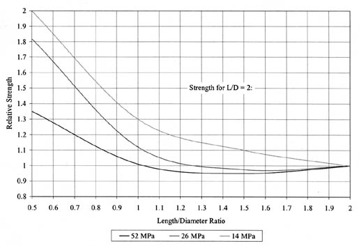
Expt. Type Layer Type LTPP Designation SHRP Protocol Minimum Number of Tests per Layer Sampling Location All GPS experiments Subgrade SS03 P43 2 TP, BA1-BA3
SPS-1 Subgrade SS03 P43 6 B1-B6
SPS-1 Embankment SS03 P43 3 B7-B12
SPS-2 Embankment SS03 P43 3 B7-B12
SPS-5 Subgrade SS03 P43 3 BA1-3, TP, BA4-6
SPS-6 Subgrade SS03 P43 3 TP1, BA1-3, TP2
SPS-8 Subgrade SS03 P43 3 B1-B3
Field Names GPS 1 through 9 SPS-1 SPS-2 SPS-5 SPS-6 SPS-8 SPS-9 State Code X X X X X X X
SHRP_ID X X X X X X X
Construction Number X X X X X X X
Layer Number X
Material Code X X X X X X
Layer type X X X X X X
Experiment Type Experiment Number Total Number of Records at All Levels Total Number of Records at Level E Percentage of Records at Level E Number of Analysis Cells Represented at Level E GPS 1 940 940 100 488
GPS 3 419 419 100 217
GPS 3 447 446 99.8 232
GPS 4 217 217 100 111
GPS 5 239 239 100 121
GPS 6 246 246 100 129
GPS 6 59 59 100 33
GPS 7 122 122 100 62
GPS 7 23 23 100 12
GPS 9 81 81 100 41
SPS 1 136 114 83.8 26
SPS 2 120 96 80.0 21
SPS 5 99 81 81.8 22
SPS 6 55 42 76.4 14
SPS 8 81 75 92.6 23
SPS 9 29 27 93.1 17
Experiment Type Number of Analysis Cells with Data and Material Information Min. Number of Test Results Required Analysis Cells with Minimum Number of Test Results Percent Analysis Cells with Minimum Test Results GPS-1 480 2 444 92.5
GPS-2 216 2 201 93.1
GPS-3 225 2 208 92.4
GPS-4 110 2 105 95.5
GPS-5 120 2 116 96.7
GPS-6A 129 2 117 90.7
GPS-6B 32 2 25 78.1
GPS-7A 60 2 58 96.7
GPS-7B 12 2 11 91.7
GPS-9 40 2 39 97.5
SPS-1 31 6/31 23 74.2
SPS-2 7 6/31 6 85.7
SPS-5 36 3 11 30.6
SPS-6 3 3 1 33.3
SPS-8 5 3 2 40.0
Soil Description Place of Origin Plastic Limit Liquid Limit Plasticity Index Bryce B Illinois 24 53 29
Cisne B Illinois 20 59 39
Cowden B Illinois 21 54 33
Drummer B Illinois 23 54 31
Elliot B Illinois 25 53 28
Fayette B Illinois 21 50 29
Hosmer B2 Illinois 24 41 17
AASHO Road Test Illinois 14 25 11
Huey B Illinois 17 46 29
Sable B Illinois 27 51 24
Limestone1 Texas 10 21 11
Iron ore gravel1 Texas 1 18 17
Sandy gravel1 Texas 7 20 13
Caliche1 Texas 15 33 18
Silt Texas 6 23 17
Lean Clay Texas 10 28 18
Fat Clay Texas 21 35 14
Lias Clay England 24 60 36
Weald clay England 25 68 43
Oxford clay England 24 72 48
London Clay England 26 78 52
Silty clay England 24 43 19
Sandy clay England 19 27 8
Clay silt England 19 33 14
Bearpaw(Cret.) Nebraska 90 130 40
Pepper (Cret.) Waco, Texas 58 80 22
Bearpaw (Cert.) Saskatchewan 92 115 23
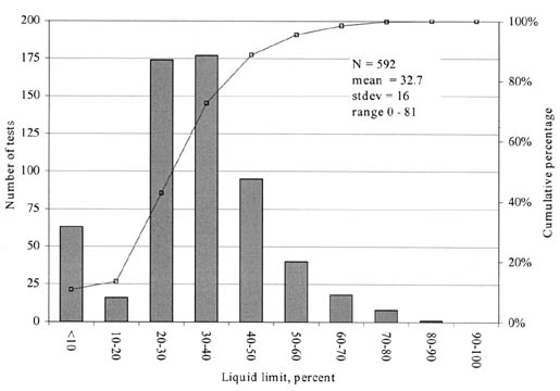
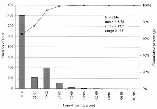
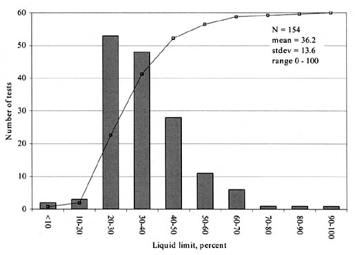
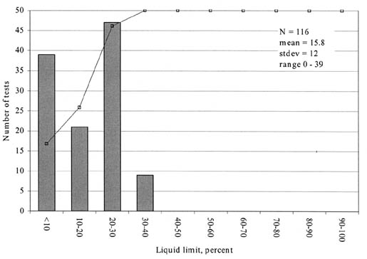
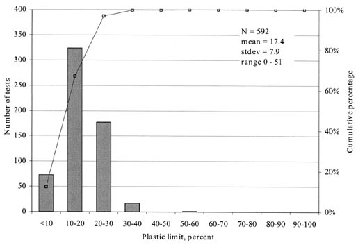
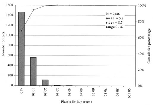
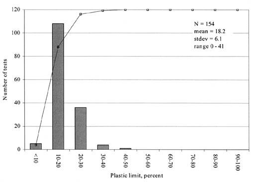
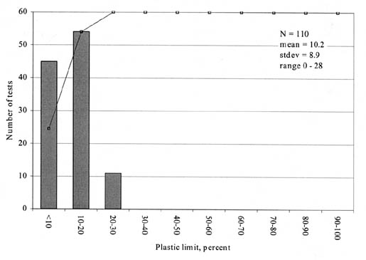
Condition of Test Liquid Limit Acceptable Range of Two Results Plastic Limit Acceptable Range of Two Results Single operator, single laboratory using the same apparatus, and on different days Less than 7 percent of mean value Less than 10 percent of mean value
Multioperators, multilaboratories Less than 13 percent of mean value Less than 18 percent of mean value
Testing Condition Test Property No. of Soils No. of Operators No. of Tests per Operator No. of Labs Avg. Standard Deviation, % Standard Deviation Range, % Avg. COV, % COV Range, % Within operator LL 3 2 10 1 0.70 0.56-0.85 2.0 1.5-2.5
Within operator PL 3 2 10 1 0.72 0.64-0.88 3.6 3.0-4.0
Within operator PI 3 2 10 1 0.84 0.64-0.99 6.0 3.7-8.7
Between operator LL 9 5 1 1 1.10 0.44-2.14 4.0 1.7-7.7
Between operator PL 9 5 1 1 1.03 0.37-2.20 6.5 2.3-13.2
Between operator PI 9 5 1 1 1.53 0.94-2.54 14.6 6.7-33.8
Between Laboratory LL 3 1 1 99 3.20 1.7-5.4 7.8 6.2-9.9
Between Laboratory PL 3 1 1 99 2.80 2.1-3.5 12.3 9.1-15.5
Between Laboratory PI 3 1 1 99 3.90 2.4-5.7 43.5 17.8-78.0
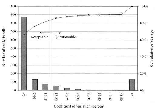
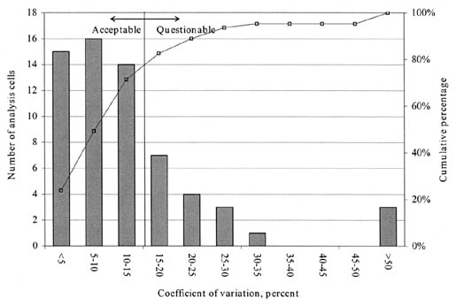
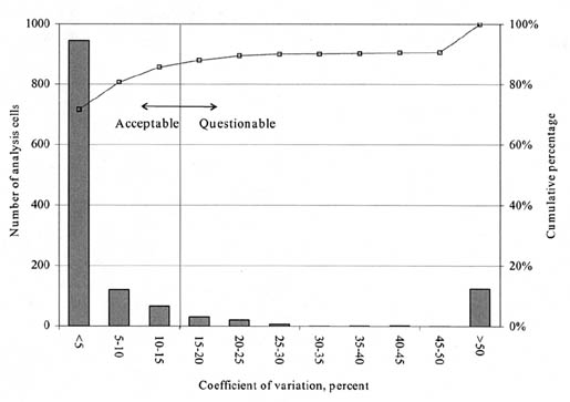
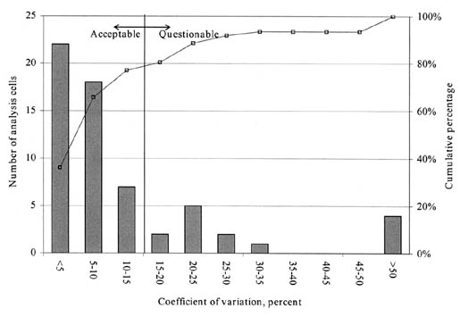
PL = plastic limit; LL = liquid limit.Code Number TST_ UG04_SS03_REP_GPS TST_ UG04_SS03_REP_SPS 1 State code State code
2 SHRP identification number SPS cell identification number
3 Layer number Description of the layer
4 Construction number Material code of the layer
5 Number of specimen tested Construction number
6 Mean LL Number of specimen tested
7 Maximum LL Mean LL
8 Minimum LL Maximum LL
9 Mean PL Minimum LL
10 Maximum PL Mean PL
11 Minimum PL Maximum PL
12 Mean PI Minimum PL
13 Maximum PI Mean PI
14 Minimum PI Maximum PI
15 Standard deviation of LL Minimum PI
16 Coefficient of variation of LL Standard deviation of LL
17 Standard deviation of PL Coefficient of variation of LL
18 Coefficient of variation of PL Standard deviation of PL
19 Standard deviation of PI Coefficient of variation of PL
20 Coefficient of variation of PI Standard deviation of PI
21 QA_Comment_1 Coefficient of variation of PI
22 QA_Comment_2 QA_Comment_1
23 QA_Comment_3 QA_Comment_2
24 QA_Comment_4 QA_Comment_3
25 QA_Comment_5 QA_Comment_4
26 QA_Comment_6 QA_Comment_5
27 QA_Comment_Other QA_Comment_6
28 Record status QA_Comment_Other
29 Record status
Expt Type Layer Type LTPP Designation LTPP Protocol Minimum Number of Tests per Layer Sampling Location SPS-1 Subgrade SS10 P54 6 A1-A18
SPS-1 Embankment SS10 P54 6 A1-A18 (if available)
SPS-2 Subgrade SS10 P54 6 A1, A4, A8, A10, A13, A16
SPS-2 Embankment SS10 P54 6 A1, A4, A8, A10, A13, A16
SPS-8 Subgrade SS10 P54 2 A2, A4
Field Names GPS 1 through 9 SPS 1 SPS 2 SPS 5 SPS 6 SPS 8 SPS 9 State Code X X X X X X X
SHRP ID X X X X X X X
Construction Number X X X X X X X
Layer Number X
Material Code X X X X X X
Layer Type X X X X X X
Expt. Type Expt. No. Total Number of Records at all Levels Total Number of Records at Level E Percentage of Records at Level E Number of Analysis Cells Represented at Level E SPS 1 54 40 74.1 7
SPS 2 29 19 65.5 6
SPS 8 11 10 90.9 4
Experiment Type Number of Analysis Cells with Data and Material Information Min. Number of Test Results Required Number of Analysis Cells with Min. Number of Test Results Percent Analysis Cells with Minimum Test Results SPS-1 7 6 3 43
SPS-2 5 6 1 20
SPS-8 4 2 3 75
Consistency of Soil Unconfined Compressive Strength, kPa Very soft <25
Soft 25-50
Medium 50-100
Stiff 100-200
Very Stiff 200-400
Hard >400
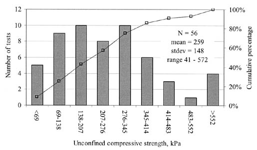
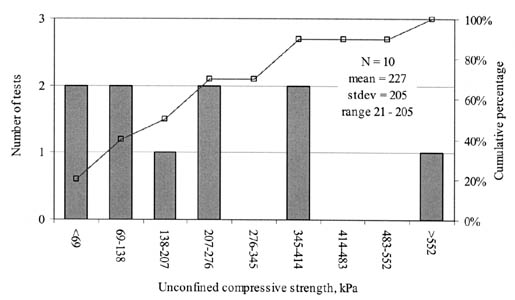
Data Source Soil Type Number of Tests Specimens per Test Avg. Standard Deviation Standard Deviation Range Avg. COV, % COV Range, % Yoder and Witzak(26) Fine-grained 40 8 5 1.5-10 8.4 1.6-26.1
Yoder and Witzak(26) Coarse-grained 12 5 21 1.7-49.2 11.2 2.6-26.8
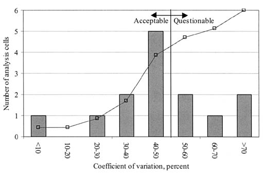
for gradation of unbound base, subbase,
and subgrade materials.
1SPS-1, -2, -5, -6, -7, -8, and -9A.Data Fields GPS SPS1 State code X X
SHRP_ID X X
Layer number X X
Layer type X X
Material code X X
Construction number X X
Experiment Type Experiment Number Total Number of Samples Tested (All QC Levels A to E) Total Number of Samples atLevel E Percent Samples at Level E Total Number of Analysis Cells Represented GPS 1 941 935 99.4 486
GPS 2 422 419 99.3 216
GPS 3 449 441 98.2 233
GPS 4 218 213 97.7 109
GPS 5 238 236 99.2 120
GPS 6A 248 248 100.0 130
GPS 6B 59 58 98.3 35
GPS 7A 124 122 98.4 62
GPS 7B 23 22 95.7 12
GPS 9 81 76 93.8 39
SPS 1 150 128 85.3 26
SPS 2 137 102 74.5 21
SPS 5 121 78 64.5 23
SPS 6 65 34 52.3 13
SPS 7 18 18 100.0 6
SPS 8 100 82 82.0 24
SPS 9 63 4 6.3 2
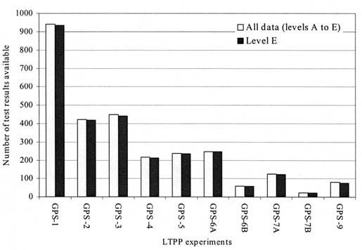
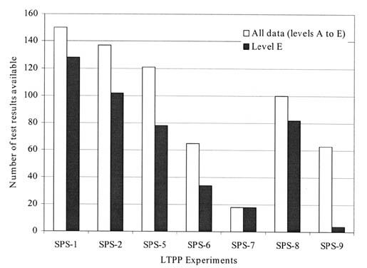
Experiment Type1 Layer Type Test Type LTPP Designation LTPP Protocol Minimum Number of Tests per Layer Sampling Location GPS 1 - 7 and 9 Base Sieve analysis UG01, UG02 P41 2 Approach end, BA, Leave end, TP1
GPS 1 - 7 and 9 Subgrade Sieve analysis SS01 P51 2 Approach end, BA, Leave end, TP1
SPS-1 Subgrade (with embankment >/= 1.2 m) No test -- -- -- --
SPS-1 Subgrade (with embankment < 1.2 m) Sieve analysis SS01 P51 6 B1-B6
SPS-1 Embankment (< 1.2 m thick) Sieve analysis SS01 P51 6 B7-B12
SPS-1 Embankment (>/= 1.2 m thick) Sieve analysis SS01 P51 6 B1-B6
SPS-1 Unbound granular base/subbase Particle size analysis UG01, UG02 P41 3 B13-B15
SPS-1 Unbound granular base/subbase Sieve analysis (washed) UG01, UG02 P41 3 B13-B15
SPS-2 Subgrade (with embankment >/= 1.2 m) No test -- -- -- --
SPS-2 Subgrade (with embankment < 1.2 m) Sieve analysis SS01 P51 6 B1-B6
SPS-2 Embankment (< 1.2 m thick) Sieve analysis SS01 P51 6 B7-B12
SPS-2 Embankment (>/= 1.2 m thick) Sieve analysis SS01 P51 6 B1-B6
SPS-2 Unbound granular base/subbase Particle size analysis UG01, UG02 P41 3 B13-B15
SPS-2 Unbound granular base/subbase Sieve analysis (washed) UG01, UG02 P41 3 B13-B15
SPS-5 Subgrade Sieve analysis SS01 P51 3 [BA1-3] [TP] [BA4-6]
SPS-5 Unbound granular base/subbase Particle size analysis UG01 P41 3 [BA1-3] [TP] [BA4-6]
SPS-5 Unbound granular base/subbase Sieve analysis (washed) UG01 P41 3 [BA1-3] [TP] [BA4-6]
SPS-6 Subgrade Sieve analysis SS01 P51 3 TP1 [BA1-3] TP2
SPS-6 Unbound granular base/subbase Particle size analysis UG01 P41 3 TP1 [BA1-3] TP2
SPS-6 Unbound granular base/subbase Sieve analysis (washed) UG01 P41 3 TP1 [BA1-3] TP2
SPS-7 Subgrade Sieve analysis SS01 P51 3 TP1 [BA1-3] TP2
SPS-7 Unbound granular base/subbase Particle size analysis UG01 P41 3 TP1 [BA1-3] TP2
SPS-7 Unbound granular base/subbase Sieve analysis (washed) UG01 P41 3 TP1 [BA1-3] TP2
SPS-8 Subgrade Sieve analysis SS01 P51 3 B1-B3
SPS-8 Unbound granular base/subbase Particle size analysis UG01 P41 3 B4-B6
SPS-8 Unbound granular base/subbase Sieve analysis (washed) UG01 P41 3 B4-B6
SPS 9 (new construction) Subgrade Sieve analysis SS01 P51 3 B01A01, B01A02, B01A03
SPS 9 (new construction) Unbound granular base/subbase Particle size analysis UG01 P41 3 B02A01, B02A02, B02A03
SPS 9 (existing construction-overlay) Subgrade Sieve analysis SS01 P51 3 A01A01, A01A02, A01A03
SPS 9 (existing construction--overlay) Unbound granular base/subbase Particle size analysis -- -- -- --
Experiment Type Total Number of Analysis Cells (Layers) Represented Number of Layers/Cells with Less Than Minimum No. of Tests Percent Layers/Cells with Incomplete Data GPS-1 486 41 8.4
GPS-2 216 16 7.4
GPS-3 233 25 10.7
GPS-4 109 5 4.6
GPS-5 120 5 4.2
GPS-6A 130 12 9.2
GPS-6B 35 8 22.9
GPS-7A 62 3 4.8
GPS-7B 12 2 16.7
GPS-9 39 2 5.1
Expt. Type Expt. Number State Code SHRP ID Construction Number Layer No. Cell/Layer Description Number of Samples Minimum No. of Samples Minimum Satisfied? S 1 1 100 1 2 Base 3 3 Yes
S 1 1 100 1 1 Subgrade 6 7 Yes
S 1 4 100 1 2 Base 3 4 Yes
S 1 4 100 1 1 Subgrade 6 12 Yes
S 1 5 100 1 1 Subgrade 6 5 No
S 1 12 100 1 2 Base 3 1 No
S 1 12 100 1 1 Subgrade 6 5 No
S 1 19 100 1 3 Base 3 3 Yes
S 1 19 100 1 2 Embankment 6 7 Yes
S 1 22 100 1 2 Embankment 6 6 Yes
S 1 22 100 1 1 Subgrade 6 6 Yes
S 1 26 100 1 2 Base 3 2 No
S 1 26 100 1 1 Subgrade 6 2 No
S 1 30 100 1 1 Subgrade 6 10 Yes
S 1 31 100 1 2 Embankment 6 3 No
S 1 31 100 1 1 Subgrade 6 5 No
S 1 32 100 1 4 Base 3 3 Yes
S 1 32 100 1 3 Embankment 6 6 Yes
S 1 32 100 1 1 Subgrade 6 6 Yes
S 1 35 100 1 1 Subgrade 6 6 Yes
S 1 40 100 1 3 Base 3 3 Yes
S 1 40 100 1 1 Subgrade 6 6 Yes
S 1 48 100 1 3 Base 3 3 Yes
S 1 48 100 1 1 Subgrade 6 6 Yes
S 1 51 100 1 3 Base 3 3 Yes
S 1 51 100 1 1 Subgrade 6 5 No
S 2 4 200 1 2 Base 3 4 Yes
S 2 4 200 1 1 Subgrade 6 9 Yes
S 2 5 200 1 2 Base 3 3 Yes
S 2 5 200 1 1 Subgrade 6 6 Yes
S 2 8 200 1 2 Base 3 3 Yes
S 2 8 200 1 1 Subgrade 6 7 Yes
S 2 10 200 1 3 Base 3 2 No
S 2 10 200 1 2 Embankment 6 5 No
S 2 10 200 1 1 Subgrade 6 16 Yes
S 2 19 200 1 3 Base 3 3 Yes
S 2 19 200 1 1 Subgrade 6 6 Yes
S 2 26 200 1 3 Base 3 3 Yes
S 2 26 200 1 2 Embankment 6 5 No
S 2 26 200 1 1 Subgrade 6 5 No
S 2 37 200 1 3 Base 3 2 No
S 2 37 200 1 2 Embankment 6 2 No
S 2 37 200 1 1 Subgrade 6 5 No
S 2 38 200 1 3 Base 3 2 No
S 2 53 200 1 4 Base 3 3 Yes
S 2 53 200 1 3 Embankment 6 9 Yes
S 2 53 200 1 2 Embankment 6 1 No
S 5 1 500 1 3 Base 3 1 No
S 5 1 500 1 1 Subgrade 3 7 Yes
S 5 4 500 1 2 Base 3 5 Yes
S 5 4 500 1 1 Subgrade 3 5 Yes
S 5 8 500 1 1 Subgrade 3 3 Yes
S 5 12 500 1 3 Base 3 1 No
S 5 13 500 1 2 Embankment 3 2 No
S 5 13 500 1 1 Subgrade 3 2 No
S 5 23 500 1 3 Base 3 7 Yes
S 5 23 500 1 2 Embankment 3 4 Yes
S 5 23 500 1 1 Subgrade 3 1 No
S 5 28 500 1, 2 1 Subgrade 3 8 Yes
S 5 30 500 1 3 Base 3 2 No
S 5 30 500 1 2 Embankment 3 2 No
S 5 30 500 1 1 Subgrade 3 2 No
S 5 34 500 1 4 Base 3 2 No
S 5 34 500 1 2 Embankment 3 3 Yes
S 5 34 500 1 1 Subgrade 3 2 No
S 5 81 500 1 2 Embankment 3 3 Yes
S 5 81 500 1 1 Subgrade 3 3 Yes
S 5 83 500 2 3 Base 3 5 Yes
S 5 83 500 2 2 Embankment 3 4 Yes
S 5 83 500 2 1 Subgrade 3 4 Yes
S 6 4 600 1 3 Treated base 3 2 No
S 6 4 600 1 2 Embankment 3 1 No
S 6 4 600 1 1 Subgrade 3 2 No
S 6 19 600 1 2 Base 3 3 Yes
S 6 19 600 1 1 Subgrade 3 3 Yes
S 6 26 600 1, 2 3 Base 3 3 Yes
S 6 29 600 1 2 Base 3 5 Yes
S 6 29 600 1 1 Subgrade 3 2 No
S 6 40 600 1 2 Base 3 3 Yes
S 6 40 600 1 1 Subgrade 3 3 Yes
S 6 42 600 2 2 Base 3 2 No
S 6 42 600 2 1 Subgrade 3 2 No
S 6 47 600 1 1 Subgrade 3 3 Yes
S 7 19 700 1, 2 3 Base 3 3 Yes
S 7 19 700 1, 2 2 Embankment 3 3 Yes
S 7 19 700 1, 2 1 Subgrade 3 3 Yes
S 7 22 700 1, 2 1 Subgrade 3 5 Yes
S 7 29 700 1, 2 2 Base 3 2 No
S 7 29 700 1, 2 1 Subgrade 3 2 No
S 8 5 800 1 3 Base 3 4 Yes
S 8 5 800 1 1 Subgrade 3 6 Yes
S 8 8 800 1 2 Base 3 3 Yes
S 8 8 800 1 1 Subgrade 3 5 Yes
S 8 30 800 1 2 Base 3 3 Yes
S 8 30 800 1 1 Subgrade 3 3 Yes
S 8 34 800 1 2 Base 3 1 No
S 8 34 800 1 1 Subgrade 3 3 Yes
S 8 36 800 1 2 Base 3 2 No
S 8 36 800 1 1 Subgrade 3 2 No
S 8 37 800 1 2 Base 3 2 No
S 8 37 800 1 1 Subgrade 3 2 No
S 8 39 800 1 3 Base 3 3 Yes
S 8 39 800 1 2 Subgrade 3 2 No
S 8 39 800 1 1 Subgrade 3 5 Yes
S 8 48 800 1 3 Base 3 3 Yes
S 8 48 800 1 1 Subgrade 3 3 Yes
S 8 49 800 1 3 Base 3 3 Yes
S 8 49 800 1 2 Embankment 3 3 Yes
S 8 49 800 1 1 Subgrade 3 3 Yes
S 8 53 800 1 4 Base 3 6 Yes
S 8 53 800 1 3 Embankment 3 6 Yes
S 8 53 800 1 2 Embankment 3 6 Yes
S 8 53 800 1 1 Subgrade 3 3 Yes
S 9 4 900 1 2 Base 3 2 No
S 9 4 900 1 1 Subgrade 3 2 No
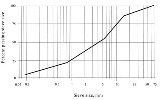
Experiment Type Total Number of Analysis Cells Number of Analysis Cells with Minimum Number of Tests Percent Analysis Cells with Complete Testing Percent Analysis Cells with Potential Sampling Bias GPS-1 486 445 91.6 8.4
GPS-2 216 200 92.6 7.4
GPS-3 233 208 89.3 10.7
GPS-4 109 104 95.4 4.6
GPS-5 120 115 95.8 4.2
GPS-6A 130 118 90.8 9.2
GPS-6B 35 27 77.1 22.9
GPS-7A 62 59 95.2 4.8
GPS-7B 12 10 83.3 16.7
GPS-9 39 37 94.9 5.1
All SPS 115 72 62.6 37.4
Total 1557 1395 89.6 10.4
Nominal Maximum Size(based on square openings), mm1 Minimum Weight of TestSample, kg 9.5 1
12.5 2
19.0 5
25.0 10
37.5 15
50 20
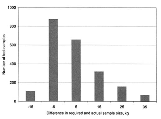
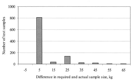
Test Condition Percent of Material between Consecutive Sieves COV (1S), Percen1, 2 Standard Deviation(1S), Percent1, 2 Single Operator3 0 to 3 304 --
Single Operator3 3 to 10 -- 1.44
Single Operator3 10 to 20 -- 0.95
Single Operator3 20 to 50 -- 1.38
Multilaboratory 0 to 3 354 --
Multilaboratory 3 to 10 -- 1.06
Multilaboratory 10 to 20 -- 1.66
Multilaboratory 20 to 30 -- 2.01
Multilaboratory 30 to 40 -- 2.44
Multilaboratory 40 to 50 -- 3.18
2The precision estimates are based on coarse aggregates with nominal maximum size of 19.5 mm.
3These values are from precision indices first included in AASHTO T27.
4AASHTO T-27 defines coarse aggregates as the fraction of material passing through the 90-mm sieve to the 9.5-mm sieve. Fine aggregates are the fraction passing through the 4.75-mm sieve to the 0.075-mm sieve.
Test Condition Percent of Material between Consecutive Sieves COV (1S), Percent1 Standard Deviation(1S) Percent1 Single Operator 0 to 3 -- 0.14
Single Operator 3 to 10 -- 0.43
Single Operator 10 to 20 -- 0.60
Single Operator 20 to 30 -- 0.64
Single Operator 30 to 40 -- 0.71
Single Operator 40 to 50 -- --
Multilaboratory 0 to 3 -- 0.21
Multilaboratory 3 to 10 -- 0.57
Multilaboratory 10 to 20 -- 0.95
Multilaboratory 20 to 30 -- 1.24
Multilaboratory 30 to 40 -- 1.41
Multilaboratory 40 to 50 -- --
Material Type Sieve Size, mm Pennsylvania Study Virginia Study Aggregate Producers North Carolina Study Virginia Producers Coarse fraction 25.4 -- 1.9 -- -- 1.8 to 2.2
Coarse fraction 19.5 3.5 to 6.8 -- 0.9 to 3.9 -- --
Coarse fraction 12.5 -- -- -- 4.3 --
Coarse fraction 9.5 5.6 to 8.3 4.2 -- -- --
Coarse fraction 4.75 5.2 to 6.2 -- 2.3 to 7.7 3.4 to 4.2 4.3 to 4.6
Fine fraction 2.36 -- -- 1.7 to 3.7 -- --
Fine fraction 2.00 -- 2.8 0.9 to 3.7 3 to 4.3 3 to 3.4
Fine fraction 1.18 3.4 to 3.6 -- -- -- --
Fine fraction 0.425 -- 1.7 -- 3.2 to 3.3 1.7 to 1.9
Fine fraction 0.250 -- -- 1.0 to 3.1 -- --
Fine fraction 0.075 1.2 to 1.4 0.9 0.7 to 1.2 1 to 1.3 0.9 to 1.1
Sieve Size, mm Number of Analysis Cells with Acceptable Variability Number of Analysis Cells with Excessive Variability Number of Analysis Cells with Single Test Data Total Number of Analysis Cells Percent Analysis Cells with Acceptable Data 75 1412 19 126 1557 90.7
50 1392 39 126 1557 89.4
37.5 1357 74 126 1557 87.2
25 1325 106 126 1557 85.1
19 1274 157 126 1557 81.8
12.5 1215 216 126 1557 78.0
9.5 1192 239 126 1557 76.6
4.75 834 597 126 1557 53.6
2 776 655 126 1557 49.8
0.425 697 734 126 1557 44.8
No. 80 734 697 126 1557 47.1
0.075 (dry) 899 532 126 1557 57.7
0.075 (wash) 890 541 126 1557 57.2
Expt. Type Expt. Number Total Number of Samples Tested (All QC Levels A to E) Total Number of Samples at Level E Total Number of Usable Samples at Level E1 Percent Usable Samples at Level E Total Number of Analysis Cells Represented GPS 1 627 624 559 89.2 288
GPS 2 473 471 459 97.0 204
GPS 3 5 5 5 100.0 3
GPS 4 2 2 0 0.0 0
GPS 6A 269 262 253 94.1 129
GPS 6B 187 184 177 94.7 80
GPS 6C 15 14 14 93.3 6
GPS 6D 4 3 3 75.0 2
GPS 6S 44 42 40 90.9 17
GPS 7A 93 92 84 90.3 44
GPS 7B 49 44 41 83.7 20
GPS 7C 2 2 2 100.0 1
GPS 7S 12 10 8 66.7 4
GPS 9 12 12 6 50.0 4
SPS 1 142 110 71 50.0 23
SPS 2 23 14 13 56.5 4
SPS 5 164 159 120 73.2 18
SPS 6 61 5 7 11.5 2
SPS 8 21 21 10 47.6 4
SPS 9 31 3 0 0.0 0
Notes:Six records were removed because they had the wrong material descriptions.
Seventeen records from SPS-5 supplemental sections were removed.
There were 141 records with material description information from table TST_LO5B at level A to D.
There were 74 test sections with no material description information from table TST_LO5B.
There were 237 records with gradation data at level A to D. This included 119 SPS supplemental sections.
There were 30 records classified at level A to D with no gradation information.
Of a total of 2,395 records in table TST_AG04, 405 were not used in any further analysis because of the reasons stated above. Statistics describing the remaining 1,990 remaining records are presented in the table.
Eighteen records at level E with materials description information had missing gradation data.
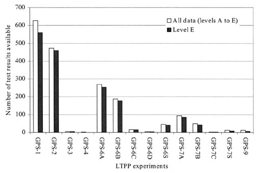
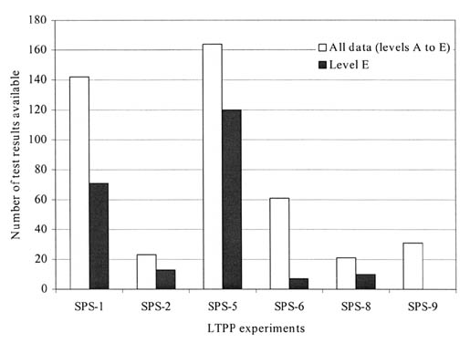
Experiment Type Layer Type LTPP Designation SHRP Protocol Minimum Number of Tests per Layer Sampling Location GPS-1, -2, -6, and -7 Asphalt Concrete AG04 P14 2 TP, BA1
SPS-1 Asphalt-Treated Base AG04 P14 3 B19, B20, B21 from paver
SPS-1 Asphalt Concrete Surface and Binder AG04 P14 3 B25, B26, B27 from paver
SPS-5 Preconstruction Asphalt Concrete AG04 P14 3 BA1-3, TP, BA4-6
SPS-5 Postconstruction Asphalt Concrete AG04 P14 6 BV1, BV2, BV3, BR1, BR2, BR3
SPS-6 Asphalt Concrete AG04 P14 3 BV1, BV2, BV3,
SPS-8 Asphalt Concrete AG04 P14 3 BV-01, BV-02, BV-03,
Experiment Type Total Number of Analysis Cells (Layers) Represented Number of Layers/Cells with Less Than Minimum Number of Tests Percent Layers/Cells with Incomplete Data GPS-1 288 16 5.6
GPS-2 204 8 3.9
GPS-3 3 1 33.3
GPS-4 0 0 0.0
GPS-6A 129 5 3.9
GPS-6B 80 8 10.0
GPS-6C 6 1 16.7
GPS-6D 2 1 50.0
GPS-6S 17 0 0.0
GPS-7A 44 4 9.1
GPS-7B 20 1 5.0
GPS-7C 1 0 0.0
GPS-7S 4 0 0.0
GPS-9 4 2 50.0
Expt. Type Expt. Number State Code SHRP ID Const. No. Layer No. Cell/Layer Material Description No. of Samples Minimum No. of Samples Minimum Satisfied? S 1 4 100 1 3 325 3 3 Yes
S 1 4 100 1 4 319 4 3 Yes
S 1 4 100 1 5 1 4 3 Yes
S 1 10 100 1 7 1 8 3 Yes
S 1 12 100 1 4 319 3 3 Yes
S 1 12 100 1 5 1 6 3 Yes
S 1 19 100 1 5 1 3 3 Yes
S 1 19 100 1 4 319 3 3 Yes
S 1 31 100 1 4 325 2 3 No
S 1 31 100 1 4 319 2 3 No
S 1 32 100 1 6 1 2 3 No
S 1 32 100 1 5 319 3 3 Yes
S 1 32 100 1 5 325 4 3 Yes
S 1 35 100 1 4 1 3 3 Yes
S 1 35 100 1 4 319 5 3 Yes
S 1 39 100 1 4 1 4 3 Yes
S 1 51 100 1 4 325 2 3 No
S 1 51 100 1 6 1 5 3 Yes
S 2 8 200 1 3 325 6 3 Yes
S 2 37 200 1 4 325 2 3 No
S 2 53 200 1 5 325 4 3 Yes
S 5 4 500 2 5 13 3 9 No
S 5 4 500 1, 2 3 1 8 9 No
S 5 8 500 2 5 13 3 9 No
S 5 8 500 1, 2 3 1 5 9 No
S 5 12 500 2 6 13 4 9 No
S 5 12 500 2 7 1 5 9 No
S 5 13 500 1 4 1 2 9 No
S 5 23 500 2 10 13 6 9 No
S 5 23 500 1, 2 6 1 26 9 Yes
S 5 24 500 1 7 2 9 9 Yes
S 5 24 500 1, 2 6 1 20 9 Yes
S 5 30 500 2 6 13 3 9 No
S 5 30 500 1, 2 4 1 5 9 No
S 5 34 500 2 8 1 3 9 No
S 5 34 500 2 8 13 9 9 Yes
S 5 81 500 2 7 13 3 9 No
S 5 81 500 1, 2 4 1 6 9 No
S 6 4 600 2 6 1 3 3 Yes
S 6 47 600 2 6 1 4 3 Yes
S 8 34 800 1 3 1 1 3 No
S 8 36 800 1 5 1 3 3 Yes
S 8 49 800 1 4 1 3 3 Yes
S 8 53 800 1 5 1 3 3 Yes
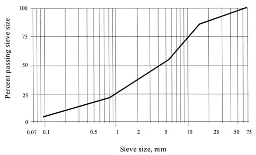
Experiment Type Total Number of Analysis Cells Number of Analysis Cells with Minimum Number of Tests Percent Analysis Cells with Complete Testing Percent Analysis Cells with Potential Sampling Bias GPS-1 288 272 94.4 5.6
GPS-2 204 196 96.1 3.9
GPS-3 3 2 66.7 33.3
GPS-4 0 0 -- --
GPS-6A 129 124 96.1 3.9
GPS-6B 80 72 90.0 10.0
GPS-6C 6 5 83.3 16.7
GPS-6D 2 1 50.0 50.0
GPS-6S 17 17 100.0 0.0
GPS-7A 44 40 90.9 9.1
GPS-7B 20 19 95.0 5.0
GPS-7C 1 1 100.0 0.0
GPS-7S 4 4 100.0 0.0
GPS-9 4 2 50.0 50.0
All SPS 44 25 56.8 43.2
Total 846 780 92.2 7.8
Test Condition Total Percentage of Material Passing a Sieve Standard Deviation (1S) Percent1, 2 Acceptable Range of Two Test Results--(D2S), Percent1, 2 Single Operator < 100 >/= 95 0.49 1.4
Single Operator < 95 >/= 40 1.06 3.0
Single Operator < 40 >/= 25 0.99 2.8
Single Operator < 25 >/= 10 0.46 1.3
Single Operator < 10 >/= 5 0.25 0.7
Single Operator < 5 >/= 2 0.21 0.6
Single Operator < 2 >/= 0 0.17 0.5
Multilaboratory < 100 >/= 95 0.57 1.6
Multilaboratory < 95 >/= 40 1.24 3.5
Multilaboratory < 40 >/= 25 0.84 2.4
Multilaboratory < 25 >/= 10 0.81 2.3
Multilaboratory < 10 >/= 5 0.56 1.6
Multilaboratory < 5 >/= 2 0.43 1.2
Multilaboratory < 2 >/= 0 0.32 0.9
2The precision estimates are based on coarse aggregates with nominal maximum size of 19.5 mm.
Sieve Size, mm Standard Deviation Arkansas Standard Deviation Washington Standard Deviation Pennsylvania Study Standard Deviation Bureau of Public Roads Standard Deviation Virginia Coarse Fraction 12.5 - 19 1.7 1.6 2.3 1.4 --
Coarse Fraction 9.5 2.6 2.5 4.4 2.5 1.9
Coarse Fraction 4.75 - 6.3 2.8 3 3.4 3.5 3.3
Fine Fraction 2 - 2.3 1.7 2.4 2.5 2.8 3.2
Fine Fraction 0.6 - 0.85 1.3 -- 1.9 2.1 2.1
Fine Fraction 0.3 - .425 1.3 1.6 1.5 1.6 1.6
Fine Fraction 0.08 - 0.3 1.1 -- 1.2 1.2 1.2
Fine Fraction 0.075 0.6 0.5 1 0.9 0.9
Sieve Size, mm Number of Analysis Cells with Acceptable Variability Number of Analysis Cells with Excessive Variability Number of Analysis Cells with Single Test Data Total Number of Analysis Cells Percent Analysis Cells with Acceptable Data 37.5 783 70 68 853 91.8
25 762 91 68 853 89.3
19 729 124 68 853 85.5
12.5 674 179 68 853 79.0
9.5 656 197 68 853 76.9
4.75 668 185 68 853 78.3
2 711 142 68 853 83.4
0.425 704 149 68 853 82.5
No. 80 744 109 68 853 87.2
0.075 764 89 68 853 89.6
Existing Table Description Representative Test Table TST_AC_01 AC core examination and thickness TST_AC01_REP
TST_AC_02 AC bulk specific gravity TST_AC_02_REP_GPS TST_AC_02_REP_SPS
TST_AC_03 AC maximum specific gravity TST_AC_03_REP_GPS TST_AC_03_REP_SPS
TST_AC_04 Asphalt content of asphaltic concrete TST_AC_04_REP_GPS TST_AC_04_REP_SPS
TST_AC05 Moisture susceptibility TST_AC05_REP
TST_AG_04 Gradation of extracted aggregate from asphaltic concrete TST_AG_04_REP
TST_PC01 Determination of compressive strength of in-place concrete TST_PC01_REP
TST_PC03 Coefficient of thermal expansion for PCC TST_PC03_REP
TST_PC06 Visual examination and length measurement of PCC cores TST_PC06_REP
TST_PC09 Flexural strength of concrete TST_PC09_REP
TST_SS01_UG01_UG02 Particle size analysis of granular base/subbase TST_SS01_UG01_UG02_REP
TST_UU04_SS03 Determination of Atterberg limits (subgrade) TST_UU04_SS03_REP_GPS TST_UU04_SS03_REP_SPS
TST_SS10 Unconfined compressive strength of subgrade soils TST_SS10_REP
TST_TB02 Unconfined compressive strength of treated base/subbase material TST_TB02_REP
Test Table in LTPP Database Level 1 Percent Records at Level E Level 1 Number of Analysis Cells Represented Level 2 Percent Cells with Minimum Tests Performed TST_PC06 89.7 551 76.2
TST_PC09 91.5 90 59
TST_PC01 83.3 432 85.1
TST_PC03 100 173 --
TST_UG01_UG02_SS01 93 1557 87.3
TST_TB02 98.1 104 90.4
TST_AC01_LAYER 99.5 3663 48.7
TST_AC02 96.8 1083 82.7
TST_AC03 96.9 962 82.8
TST_AC04 99.3 968 83.7
TST_AG04 92.9 853 92.1
TST_SS03 97.4 1569 87.1
TST_AC05 55.7 23 26.1
TST_SS10 73.4 17 41.2
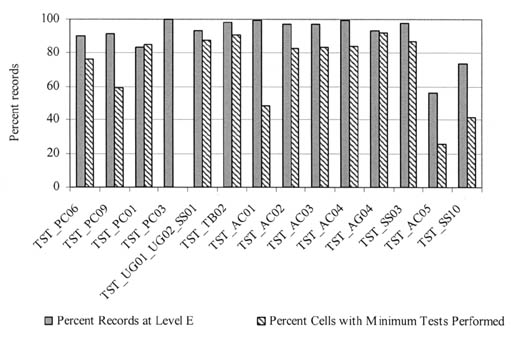
Category Criteria Test Tables I "Good" level 1 data completeness--80 to 100 percent of total test data (from all levels) is at level E. TST_PC01, TST_UG01_UG02_SS01,TST_TB02, TST_AC02, TST_AC03, TST_AC04, TST_AG04, TST_SS03
I "Good" level 2 data completeness--80 to 100 percent data has adequate sampling TST_PC01, TST_UG01_UG02_SS01,TST_TB02, TST_AC02, TST_AC03, TST_AC04, TST_AG04, TST_SS03
II "Poor" to "Fair" level 1 data completeness--0 to 80 percent of total test data (from all levels) is at level E. --
II "Good" level 2 data completeness--80 to 100 percent data has adequate sampling. --
III "Good" level 1 data completeness--80 to 100 percent of total test data (from all levels) is at level E. TST_PC06, TST_PC09, TST_AC01
III "Poor" to "Fair" level 2 data completeness--0 to 80 percent data has adequate sampling. TST_PC06, TST_PC09, TST_AC01
IV "Poor" to "Fair" level 1 data completeness--0 to 80 percent of total test data (from all levels) is at level E. TST_AC05, TST_SS10
IV "Poor" to "Fair" level 2 data completeness--0 to 80 percent data has adequate sampling. TST_AC05, TST_SS10
materials.