U.S. Department of Transportation
Federal Highway Administration
1200 New Jersey Avenue, SE
Washington, DC 20590
202-366-4000
Federal Highway Administration Research and Technology
Coordinating, Developing, and Delivering Highway Transportation Innovations
 |
| This report is an archived publication and may contain dated technical, contact, and link information |
|
Publication Number: FHWA-RD-03-041 |
Previous | Table of Contents | Next
This chapter contains the results of an evaluation of within-section variation in layer thickness values. Characteristics of within-section layer thickness variability are very important inputs in reliability-based pavement engineering applications. This chapter contains the discussion of data sources used for the analysis of within-section variation in layer thickness values, the methodology used to assess characteristics of within-section layer thickness distribution, testing procedures used to evaluate goodness-of-fit between theoretical models and observed layer thickness data, and the results of the within-section layer thickness variability evaluation.
Data from the elevation measurements were used to evaluate the extent of within-section variation in layer thicknesses. Elevation measurements for each pavement layer were taken along the LTPP section length during the construction phase of the SPS experiments. These data are available in the SPS*_LAYER_THICKNESS tables. Unlike other LTPP layer thickness tables, the data in the SPS*_LAYER_THICKNESS tables are stored not by the layer number but by layer and material type identifiers. Table 30 provides an overview of which identifiers are available in the SPS*_LAYER_THICKNESS tables.
| Layer and Material Type | LTPP Field Name (layer identifier) | LTPP Table Name |
|---|---|---|
| AC surface course | SURFACE_COURSE | SPS5_LAYER_THICKNESS, SPS6_LAYER_THICKNESS |
| AC binder course | BINDER_COURSE | SPS5_LAYER_THICKNESS, SPS6_LAYER_THICKNESS |
| AC surface and binder course | SURFACE_AND_BINDER | SPS1_LAYER_THICKNESS |
| ASPH_SURFACE_AND_BINDER | SPS8_LAYER_THICKNESS | |
| AC surface friction course | SURFACE_FRICTION | SPS1_LAYER_THICKNESS, SPS5_LAYER_THICKNESS, SPS6_LAYER_THICKNESS, SPS8_LAYER_THICKNESS |
| DGAB | DENSE_GRADE_AGG_BASE | SPS1_LAYER_THICKNESS, SPS2_LAYER_THICKNESS, SPS8_LAYER_THICKNESS |
| DGATB | DENSE_GRD_ASPH_TREAT_BASE | SPS1_LAYER_THICKNESS |
| PATB | PERM_ASPH_TREAT_BASE | SPS1_LAYER_THICKNESS, SPS2_LAYER_THICKNESS |
| LC base | LEAN_CONCRETE | SPS2_LAYER_THICKNESS |
| PCC surface layer | PCC_SURFACE | SPS2_LAYER_THICKNESS |
| PORT_CEMENT_CONCRETE_SURFACE | SPS8_LAYER_THICKNESS | |
| PCC overlay layer | SURFACE_COURSE | SPS7_LAYER_THICKNESS |
| Rut level-up layer | RUT_LEVEL_UP | SPS5_LAYER_THICKNESS, SPS6_LAYER_THICKNESS |
| Mill replacement layer | MILL_REPLACE | SPS5_LAYER_THICKNESS, SPS6_LAYER_THICKNESS |
Design Thickness
For a particular SPS experiment, several design thickness values were used as a target design layer thickness. For a given SPS section, only one design thickness value was used along the section length. The design thicknesses for different layers were reviewed for each SPS experiment. Table 31 provides an overview of the material and layer types used in different SPS experiments, the design thicknesses, and the number of layers with the along-the-section thickness measurements available in the LTPP database, Level E version released on June 29, 2001.
Descriptive Layer Thickness Statistics
Using layer thickness measurements along the section, an exploratory data analysis was conducted, and descriptive statistical measures such as mean, standard deviation, kurtosis, skewness, and number of thickness measurements per layer were computed for each structural layer (surface and base courses) that had layer thickness information available in the SPS*_LAYER_THICKNESS tables. These descriptive statistics were then used to evaluate characteristics of layer thickness distribution along the LTPP section.
The following description of the statistical variables provides background information to facilitate the understanding of the procedures used to evaluate within-project layer thickness variability.
The mean is a property of the distribution that describes the location of the distribution. The mean layer thickness is computed as the average of the individual thicknesses obtained from elevation measurements taken along the LTPP section.
The standard deviation is a property of the distribution that describes the spread of the distribution. The standard deviation is based on the second moment of the measurement distribution.
The skewness is a property of the distribution that is used to evaluate how skew the distribution is. The skewness is 0 for a symmetric distribution, positive if the distribution has a long tail to the right, and negative if the distribution has a long tail to the left. The skewness is based on the third moment of the measurement distribution.
The kurtosis is another property of the distribution that provides a mean to evaluate how heavy (or light) the tails of the distribution are. For a normal distribution, the kurtosis is 0. For a distribution with long or fat tails, the kurtosis is positive. For a distribution with short or slim tails, relative to a normal distribution, the kurtosis is negative (but always > -3). The adjusted fourth moment of the measurement distribution is one way to measure the kurtosis of the distribution.
| Layer and Material | Type Experiment | Type Design Layer Thickness, mm (in) | Total Number of Layers used in the Analysis |
|---|---|---|---|
| AC surface course | SPS-5 | 0 | 93 |
| 51 (2) | |||
| 127 (5) | |||
| SPS-6 | 0 | 40 | |
| 102 (4) | |||
| 203 (8) | |||
| AC surface and binder course | SPS-1 | 102 (4) | 167 |
| 178 (7) | |||
| SPS-8 | 102 (4) | 24 | |
| 178 (7) | |||
| AC binder course | SPS-5 | Varies | 33 |
| SPS-6 | Varies | 17 | |
| DGAB | SPS-1 | 102 (4) | 97 |
| 2023 (8) | |||
| 305 (12) | |||
| SPS-2 | 102 (4) | 85 | |
| 152 (6) | |||
| SPS-8 | 152 (6) | 38 | |
| 203 (8) | |||
| 305 (12) | |||
| DGATB | SPS-1 | 102 (4) | 97 |
| 203 (8) | |||
| 305 (12) | |||
| PATB | SPS-1 | 102 (4) | 83 |
| SPS-2 | 102 (4) | 47 | |
| LC base | SPS-2 | 152 (6) | 48 |
| PCC surface layer | SPS-2 | 203 (8) | 140 |
| 279 (11) | |||
| SPS-8 | 203 (8) | 14 | |
| 279 (11) | |||
| PCC overlay layer | SPS-7 | 76 (3) | 24 |
| 127 (5) |
The skewness and kurtosis are two main properties of a distribution that together describe the shape of the distribution, while the mean describes the location and the standard deviation the spread of the distribution. These statistical measures were used then to determine the extent to which the variation of layer thickness along the section follows normal distribution.
Identification of Suspect Layer Thickness Data
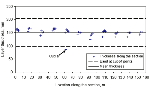
Before the analysis of the within-section layer thickness variability, layer thickness data were reviewed to identify any anomalous thickness measurements along the section. The purpose was to identify outliers - the data points that appear not to belong with the rest of the data. Figure 19 shows an obvious example.
Methodology to Identify Outliers
Because outliers can have a strong influence on both the skewness and kurtosis calculated for a data sample, the presence of a few outliers in a sample from a normal distribution may cause the sample to fail a normality test. Therefore, it is important to determine whether the apparent non-normality might be due to the presence of outliers. A data point was considered an outlier and removed from the analysis if the following is true:
The criterion is shown in equation format in figure 20.
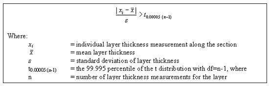
The t-values at the 99.995 percentile correspond to a level of significance of 0.01 percent for the two-sided t-test. The choice of a significance level of 0.01 percent is very conservative and was based on the fact that only "true" outliers (i.e., those that clearly do not belong in the same population with the other data points) should be excluded. If the distribution in reality is skewed, it is not desirable to cut out values based on a higher significance level, since the cut-off points are based on the (symmetric) normal distribution.
Note that the commonly used criterion (mean +/- 2 standard deviations) for identification of outliers was not used in this study. That criterion is based on a 5 percent significance level and the assumption that the distribution of the sample is normal. Because the standard deviation for LTPP sections is not known but estimated, the assumption of normality leads to the use of the t-distribution to create the 95 percent confidence interval. Based on the sample size, the t-distribution will provide a different number that the standard deviation is multiplied by to determine the cut-off points for outliers, as the examples in table 32 show.
| Sample Size | Degrees of Freedom | Multiplier for the Standard Deviation |
|---|---|---|
| 11 | 10 | 2.23 |
| 21 | 20 | 2.09 |
| 29 | 28 | 2.045 |
| 121 | 120 | 1.98 |
| ∞ | ∞ | 1.96 |
The following example using data from SPS-6 Section 40_0608 demonstrates the methodology and rationale used to determine the outlier points. The descriptive statistics for the binder course layer used in this example are provided in table 33. A scatter plot of all the thickness measurements is shown in figure 19.
| Section ID | Layer Type | Number of Layer Thickness Measurements | Mean Layer Thickness, mm (in) | Standard Deviation of Layer Thickness, mm (in) |
|---|---|---|---|---|
| 40_0608 | binder course | 55 | 151 (5.951) | 13 (0.501) |
The data point identified as "Outlier" in figure 19 was evaluated to identify whether this point is a true outlier. The layer thickness value for this point is 86 mm (3.4 in), while the mean value for the sample is 151 mm (5.951 in). Using the criterion shown in figure 20, for the left side of the expression, we obtain the t-statistic value of 5.1. For the right side of the expression, the t-value of 4.2 was obtained at the 99.995 percentile of the t distribution with 54 (df = 55-1) degrees of freedom. Since the t-statistic of 5.1 is greater than the t-value of 4.2, this point was found to be an outlier using a cut-off point based on the t-distribution at a significance level of 0.01 percent with n-1degrees of freedom.
For the data in figure 19, the outlier point at 86 mm (3.4 in) could have been as large as 97 mm (3.8 in) and still would have been removed. In this particular data set, it may be desirable to remove points even greater than 97 mm (3.8 in) because the data otherwise do not appear skewed. However, in the data sets where some skewness is present, removal of the data points on the outskirts of the distribution could bias the reliability of the distribution evaluation results. The following example is used to demonstrate this concern.
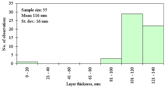
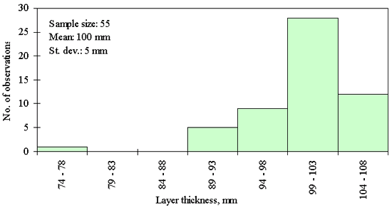
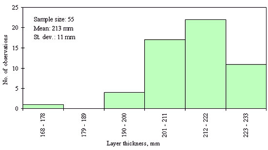
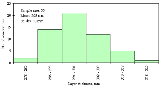
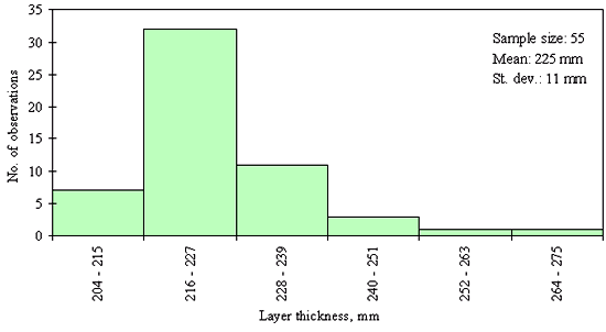
Three different layer thickness frequency distributions are presented in figures 21, 22, and 23. The distribution in figure 21 shows an example of the clear outlier point on the left side of the distribution. Here the layer thickness value of the outlying point is <20 mm, while layer thicknesses for the rest of the points range from 82 to 142 mm. However, for the figures 22 and 23, the question whether the leftmost point is an outlier, cannot be answered with the same degree of certainty. The leftmost point in the distribution provided in figure 22 is a questionable outlier. Here the layer thickness value of the outlying point is about 75 percent of the average of the layer thickness values of the other points. The leftmost point in the distribution provided in figure 23 may be a legitimate point of a skewed distribution. Here the layer thickness value of the outlying point is about 80 percent of the average of the layer thickness values of the other points. However, even at the very conservative level chosen, the outlying point in figure 22 was identified as an outlier while the outlying point in figure 23 was not. This example illustrates why it was necessary to set the level for declaring a point an outlier very conservatively (in order to not bias the analysis of distribution type) in this study.
This procedure for identification of the outliers was applied to each SPS structural layer with data available in the SPS*_LAYER_THICKNESS tables. In the whole data set of more than 55,000 data points, only 20 data points were excluded based on this criterion; the list of these excluded points is presented in table 34. These individual layer thicknesses were analyzed using special data distribution plots. The results show that these thickness values are likely to be errors in the database rather than actual thickness measurements. However, the review of the actual field data is required to confirm this conclusion. All anomalous or suspect data thickness values were reported back to the LTPP administrators for data review and possible correction of the thickness values in the LTPP layer thickness data tables.
| Exp. Type | STATE_CODE | SHRP_ID | Type | Measured Thickness (outlier), mm | Mean Thickness (with outliers), mm | St. dev. (with outliers), mm | Number of Measurements | Standardized Difference | t-value at 95.995 percent |
|---|---|---|---|---|---|---|---|---|---|
| SPS-6 | 40 | 0608 | BC | 86 | 151 | 13 | 55 | 5.09 | 4.20 |
| SPS-1 | 12 | 0102 | DGAB | 208 | 307 | 15 | 55 | 6.69 | 4.20 |
| SPS-1 | 30 | 0113 | DGAB | 102 | 210 | 24 | 55 | 4.55 | 4.20 |
| SPS-2 | 20 | 0210 | DGAB | 76 | 100 | 5 | 55 | 4.41 | 4.20 |
| SPS-1 | 5 | 0122 | DGATB | 25 | 97 | 12 | 55 | 6.03 | 4.20 |
| SPS-1 | 32 | 0105 | DGATB | 150 | 123 | 5 | 55 | 5.03 | 4.20 |
| SPS-1 | 35 | 0104 | DGATB | 193 | 297 | 25 | 55 | 4.23 | 4.20 |
| SPS-1 | 40 | 0116 | DGATB | 71 | 304 | 35 | 55 | 6.63 | 4.20 |
| SPS-2 | 5 | 0215 | PCCS | 328 | 275 | 12 | 55 | 4.31 | 4.20 |
| SPS-1 | 4 | 0116 | SB | 122 | 95 | 6 | 55 | 4.34 | 4.20 |
| SPS-1 | 10 | 0103 | SB | 46 | 121 | 12 | 55 | 6.14 | 4.20 |
| SPS-1 | 30 | 0122 | SB | 18 | 116 | 16 | 55 | 6.21 | 4.20 |
| SPS-1 | 35 | 0105 | SB | 170 | 119 | 12 | 55 | 4.24 | 4.20 |
| SPS-1 | 39 | 0105 | SB | 41 | 101 | 11 | 55 | 5.57 | 4.20 |
| SPS-1 | 51 | 0116 | SB | 33 | 73 | 9 | 55 | 4.22 | 4.20 |
| SPS-8 | 29 | A802 | SB | 142 | 174 | 7 | 63 | 4.23 | 4.16 |
| SPS-8 | 39 | 0803 | SB | 185 | 101 | 15 | 55 | 5.43 | 4.20 |
| SPS-8 | 49 | 0803 | SB | 58 | 107 | 11 | 55 | 4.29 | 4.20 |
| SPS-6 | 29 | A606 | SC | 36 | 110 | 13 | 55 | 5.71 | 4.20 |
| SPS-6 | 29 | 0608 | SC | 119 | 59 | 12 | 50 | 5.06 | 4.24 |
Formulation of Statistical Hypothesis
Goodness-of-fit tests are used to evaluate how close the experimental data follow the assumed theoretical distribution. If the targeted theoretical distribution is a "normal" distribution, then the goodness-of-fit test becomes the test for normality. Such a test evaluates the closeness of the experimental data distribution to the normal distribution.
In the goodness-of-fit test, the null and alternative hypotheses are established first:
There are two kinds of errors that can be made in testing the hypothesis:
In the test of a hypothesis, it is desirable to have a small type I error and large power. Power is equal to 1 minus probability of a type II error and is defined as the probability of rejecting the null hypothesis when the alternative hypothesis is true. Testing whether a measured variable follows a certain theoretical distribution is not straightforward in the sense that the various tests are only powerful against certain types of alternative distributions.
Selection of the Targeted Theoretical Distribution
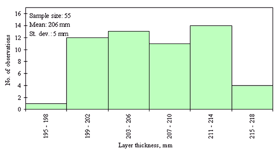
Based on the assumption that thickness measurements follow the same kind of distribution for any layer, one type of distribution was looked for. To determine the likely distribution shape, the measures of skewness and kurtosis were evaluated. The skewness of all samples ranged from -2.45 to +3.92 with a median of 0.024, while the kurtosis of all samples ranged from -1.56 to +17.78 with a median of -0.033. These measures indicate no particular skewness to either side or either particular long or short tails. This observation was confirmed by inspection of the layer thickness frequency distributions of each sample. While most of the reviewed layer thickness distributions looked fairly normal, as shown in figure 24, some samples had distributions that were skewed to one side or the other side, or looked rather uniformly distributed. Examples of different distribution shapes observed for the LTPP layer thickness measurements are provided in figures 23 to 26. The normal distribution was therefore selected as the most likely theoretical distribution to describe variability in the layer thickness along the LTPP section. This hypothesis was then tested using a goodness-of-fit test.
Selection of Testing Procedure
The goodness-of-fit test between assumed theoretical distribution and distribution of the observed data could be done using several methods including:
For the normal distribution more goodness-of-fit methods are available, including:
To select the best applicable testing procedure, the LTPP layer thickness data characteristics were analyzed first. Based on the data review the following was established:
The assumptions and requirements of different goodness-of-fit tests were reviewed from the point of their applicability and the robustness of the procedure when it is applied to the LTPP layer thickness data. The goal of this review was to find a procedure that could be uniformly used for all the sections with variable number of data points without compromising the test accuracy and without violating any of the underlying test assumptions.
For most theoretical distributions, the choice is limited to tests like the Kolmogorov-Smirnov test or the chi-square goodness-of-fit test [32]. The advantage of the Kolmogorov-Smirnov test is that unlike the chi-square test it does not have strict rules on the required number of data groups and minimum theoretical frequencies that have to be satisfied in order for the test to be meaningful. The Kolmogorov-Smirnov test could be done for the samples with as few as five observations. The Kolmogorov-Smirnov test is also more powerful than the chi-square test.
If the null hypothesis is that the measured variable follows a normal distribution, there are more powerful tests available, such as the Shapiro-Wilk's test [33], the test of skewness or the third sample moment test and the test of kurtosis or the fourth sample moment test [34]. The latter two tests work for a sample with nine observations or more. These tests are preferred to the Kolmogorov-Smirnov test because of the increased power [34] they provide. For a test to work well, it should have high power against all possible alternatives, which is not true for either the Kolmogorov-Smirnov test or the chi-square goodness-of-fit test. For the LTPP layer thickness data the Shapiro-Wilk's test was not appropriate, due to the many thickness measurement values that were the same (many "ties" [34]) for a given pavement layer and LTPP section.
The following table 35 provides a summary of the pros and cons of the reviewed goodness-of-fit testing methods.
| Evaluation Criteria | Chi-Square test | Kolmogorov-Smirnov test | Sharpiro-Wilk test | Skewness-and-Kurtosis test |
|---|---|---|---|---|
| Test power (for normality only) | very poor | poor | high | high |
| Minimum number of observations | 25 | 5 | 3 | 9 |
| Minimum number of observations in a single bin | 5 | no restriction | no restriction | no restriction |
| Handling of "ties" | high | high | poor | high |
Based on the review of different goodness-of-fit tests' procedures and analysis of the available layer thickness data, the following conclusions were derived:
The combined skewness and kurtosis test was selected for the evaluation of layer thickness distribution normality. Rejection in either skewness or kurtosis test was considered as a rejection of normality altogether. For example, for a sample to be considered as normally distributed, the analysis of data should pass both the skewness and the kurtosis tests for a selected level of significance.
Selection of the Level of Significance
The level of significance of 1 percent was chosen for the goodness-of-fit tests. The following considerations were taken into account in selecting this desired level of significance:
Procedures for the Skewness and Kurtosis Test
Based on the assessment of the LTPP layer thickness data from the SPS*_LAYER_THICKNESS tables, a procedure based on the combination of skewness and kurtosis tests was selected as the most appropriate for ascertaining whether the frequency distributions of layer thickness measurements taken along the LTPP section follow a normal distribution. In this procedure, for a sample not to be rejected (as normally distributed), the layer thickness measurements sample should pass both the skewness and the kurtosis tests for a selected level of significance of 1 percent.
The procedure used for the combined skewness and kurtosis test is outlined in the flowchart in figure 27. Detailed statistical formula used to compute test parameters are provided in Appendix B.
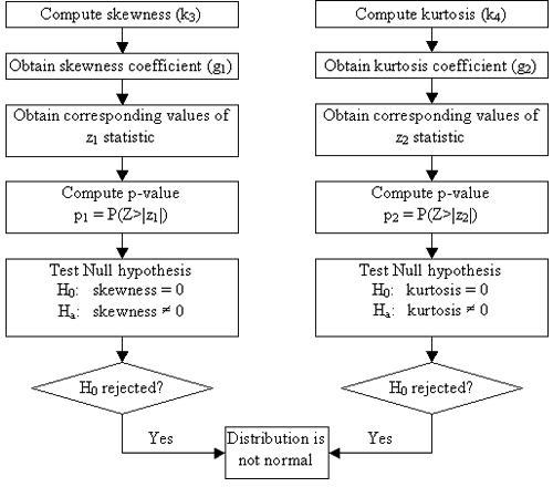
The skewness and kurtosis tests are based on evaluations of the third and fourth moments of the measurement distribution. The distribution is not rejected for being normally distributed if the absolute values of the z1- and z2-statistics computed separately based on skewness and kurtosis values are less than the Z-value of 2.57.
Z-value is obtained from the standard normal distribution, assuming a 1 percent level of significance. If a sample follows the standard normal distribution, the value Z=2.57 describes the distribution with 0.5 percent of the all the values from the sample greater than 2.57 and 0.5 percent of the values smaller than -2.57. Thus, when Z is equal to 2.57 the level of significance is 1 percent.
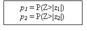
The z1- and z2-statistics are used to obtain the p-values (the probability that values of the standard normal distribution are more extreme than the computed z1- and z2-statistics). The p-values are defined in figure 28, as follows.
Based on the selected 1 percent level of significance, if p1- and p2-values are larger than 1 percent or equivalently if |z1| and |z2| < 2.57, we fail to reject that the data follow a normal distribution.
Example of the Kurtosis and Skewness Tests
The following example provides the comparison of the kurtosis and skewness test results obtained for the same binder course layer in the SPS-6 Section 40_0608, including and excluding an obvious outlier thickness measurement (86-mm [3.4-in] outlier thickness for a sample with 151-mm [5.951-in] mean thickness). Table 36 provides the summary of the test results.
| Sample Characteristic | Sample Size, n | Mean Sample Thickness,mm | Standard Deviation, mm | g1 | g2 | z1 | z2 | Z-value | Is Normal? |
|---|---|---|---|---|---|---|---|---|---|
| Outlier included in the analysis | 55 | 151.15 | 12.72 | -2.60 | 11.74 | -5.51 | 4.80 | 2.57 | No |
| Outlier excluded from the analysis | 54 | 152.35 | 9.17 | -0.57 | 0.68 | -1.77 | 1.14 | 2.57 | Yes |
When the outlier point was excluded, the mean does not change much while the standard deviation becomes 0.7 times smaller, and the skewness (g1) and the kurtosis (g2) change considerably. For this example, the exclusion of the outlying data point means that the tests for normality change from reject to not reject.
Results of the Kurtosis and Skewness Test of Normality for SPS Structural Layers
Kurtosis and skewness tests of normality were used to evaluate whether the experimental layer thickness data follow the theoretical normal distribution. A total of 1,047 layer thickness samples from the SPS experiments were considered for the analysis. Based on the number of available observations per sample, 13 samples were excluded from the analysis. These samples had fewer than 9 observations-the minimum number required for the kurtosis and skewness tests. All the samples were tested assuming the same evaluation criterion at 1 percent level of significance. The procedure for the kurtosis and skewness tests of normality described in the previous section was utilized.
The results of the kurtosis and skewness tests for different pavement material and layer types indicate that, based on the selected 1 percent level of significance, overall 84 percent of all layer thickness frequency distributions were not rejected for being normally distributed. This finding indicates that in general it is reasonable to assume that the layer thickness measurements taken along the section are normally distributed, but in a small number of sections this is not so. The distribution normality evaluations are summarized in table 37 by SPS experiment number and by layer and material type, respectively.
| Experiment | Number of Layers | Not Rejected (Normal) | Rejected (Not Normal) |
|---|---|---|---|
| AC_SURFACE_COURSE | |||
| SPS-5 | 93 | 78 (83.9 %) | 15 (16.1 %) |
| SPS-6 | 36 | 30 (83.3 %) | 6 (16.7 %) |
| SURFACE_AND_BINDER | |||
| SPS-1 | 167 | 136 (81.4 %) | 31 (18.6 %) |
| SPS-8 | 22 | 20 (90.9 %) | 2 (9.1 %) |
| PERM_ASPH_TREAT_BASE | |||
| SPS-1 | 83 | 72 (86.8 %) | 11 (13.2 %) |
| SPS-2 | 46 | 41 (89.1 %) | 5 (10.9 %) |
| PCC_SURFACE | |||
| SPS-2 | 139 | 102 (73.4 %) | 37 (26.6 %) |
| SPS-7 | 24 | 23 (95.8 %) | 1 (4.2 %) |
| SPS-8 | 14 | 12 (85.7 %) | 2 (14.3 %) |
| LEAN_CONCRETE | |||
| SPS-2 | 48 | 40 (83.3 %) | 8 (16.7 %) |
| DENSE_GRD_ASPH_TREAT_BASE | |||
| SPS-1 | 97 | 87 (89.7 %) | 10 (10.3 %) |
| DENSE_GRADE_AGG_BASE | |||
| SPS-1 | 97 | 84 (86.6 %) | 13 (13.4 %) |
| SPS-2 | 84 | 70 (83.3 %) | 14 (15.5 %) |
| SPS-8 | 38 | 30 (79.0 %) | 8 (21.0 %) |
| BINDER_COURSE | |||
| SPS-5 | 33 | 30 (87.9 %) | 3 (12.1 %) |
| SPS-6 | 13 | 12 (92.3 %) | 1 (7.7 %) |
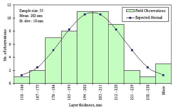
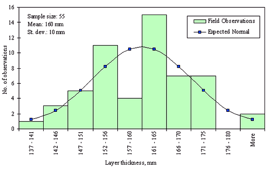
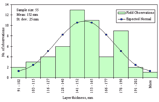
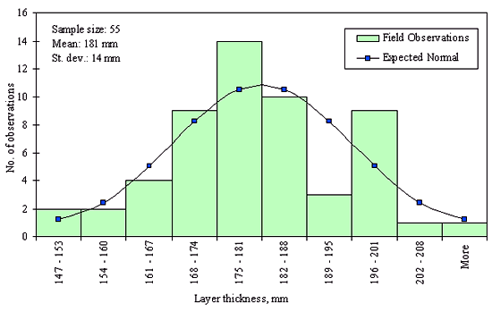
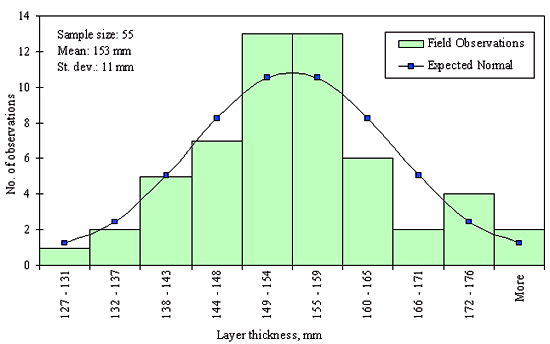
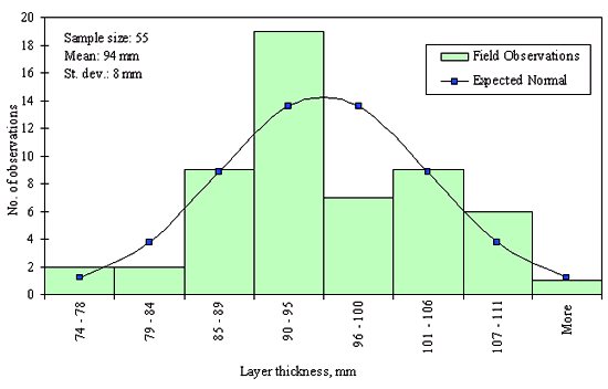
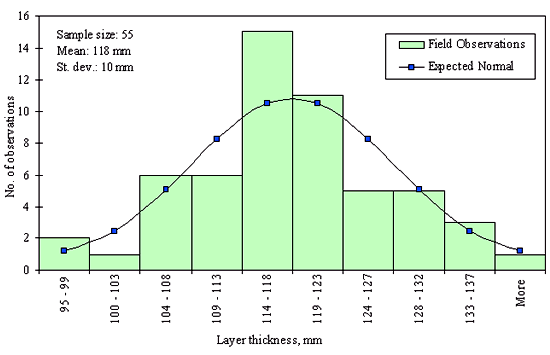
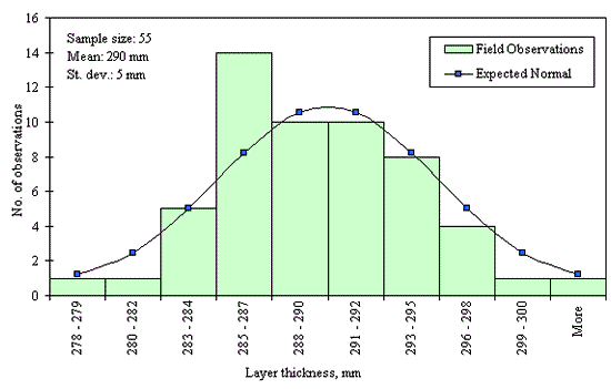
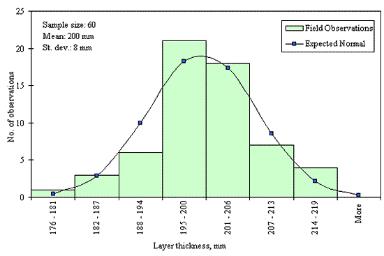
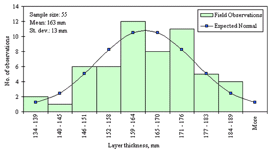
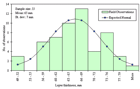
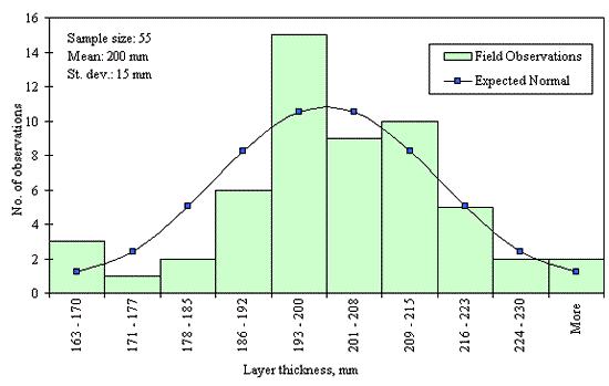
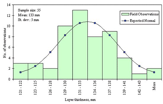
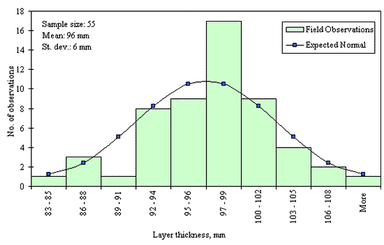
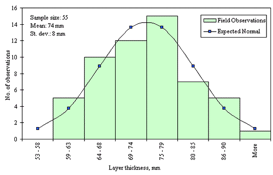
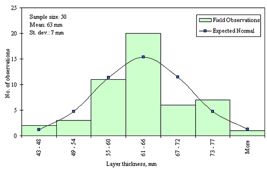
Figures 29 through 44 provide examples of layer thickness frequency distributions obtained from the elevation measurements data for different layer and material types evaluated in the goodness-of-fit study. The data used to create these frequency distributions were determined to be reasonably normal based on skewness and kurtosis tests at selected level of significance. Theoretical normal distributions are superimposed over field frequency data to provide means for visual comparison between field data and theoretical distributions.
In addition to the kurtosis and skewness tests, Kolmogorov-Smirnov goodness-of-fit tests were carried out for the layer with thickness data in the SPS*_LAYER_THICKNESS tables. As was discussed earlier in the chapter, this testing procedure is not as powerful for testing normality as the kurtosis and skewness tests. A summary of the Kolmogorov-Smirnov goodness-of-fit testing procedure and evaluation results are presented in the Appendix C.
In this chapter, layer thickness data from the SPS elevation measurements were analyzed to determine the extent to which the variation of layer thickness within a section follows typical statistical distributions. Data from the SPS*_LAYER_THICKNESS tables were obtained and reviewed. The layers used in the analysis include different material types and functional classifications, such as AC surface courses, combined AC surface and binder courses, AC binder courses, DGAB's, ATB's, LC bases, PCC surface layers, and PCC overlay layers. A methodology for identifying anomalous outlier points based on t-distribution was developed and utilized in evaluation of layer thickness data for each layer in the SPS*_LAYER_THICKNESS tables. All identified anomalous outlier data points were analyzed and reported to FHWA.
To assess layer thickness distribution characteristics, descriptive statistics such as mean, standard deviation, skewness, and kurtosis were computed for each section. Using descriptive statistics, the analysis of likely shapes of layer thickness distribution was conducted. The results of exploratory analysis indicated that, for most of the sections, the distribution is likely to be normal. To perform a more rigorous test of distribution normality, available procedures for goodness-of-fit tests were reviewed and their applicability to the evaluation of layer thickness data was evaluated. Based on the literature review, a combined test for skewness and kurtosis was selected to test normality of layer thickness distribution. A summary of the testing procedure was documented in this chapter. The analysis results for 1,034 SPS layers indicated that for 84 percent of all layer, frequency distributions of thickness values were not rejected for being normally distributed. Thus, LTPP data indicate that layer thickness variation within a section follows a normal distribution in most cases. These results would serve as a very important input to pavement engineering applications involving design reliability implementation.

