U.S. Department of Transportation
Federal Highway Administration
1200 New Jersey Avenue, SE
Washington, DC 20590
202-366-4000
Federal Highway Administration Research and Technology
Coordinating, Developing, and Delivering Highway Transportation Innovations
 |
| This report is an archived publication and may contain dated technical, contact, and link information |
|
Publication Number: FHWA-RD-02-095 Date: |
Previous | Table of Contents | Next
In comparing two sets of data, such as contractor and agency test results, what is involved is two hypothesis tests, where the Ho for each test is that the data sets are from the same population. In other words, the null hypotheses are that the variabilities of the two data sets are equal, for the F-test, and that the means of the two data sets are equal, for the t-test.
When comparing two data sets, it is important to compare both the means and the variances. A different test is used for each of these comparisons. The F-test provides a method for comparing the variances (standard deviation squared) of the two sets of data. Differences in means are assessed by the t-test. Construction processes and material properties usually follow a normal distribution. For normal distributions, the ratios of variances follow an F-distribution, while the means of relatively small samples follow a t-distribution. Hypothesis tests for equal variances and means can therefore be conducted using these distributions.
For samples from the same normal population, the statistic F, which
is the ratio of the two sample variances, has a sampling distribution called
the F-distribution. Tables are available for the F-distribution
just like they are for the normal distribution. For process verification testing,
the F-test is based on the ratio of the sample variance of the contractor's
test results, ![]() ,
and the sample variance of the agency's test results,
,
and the sample variance of the agency's test results, ![]() .
.
Similarly, the t-statistic and the t-test can be used to
test whether the sample mean of the contractor's test results, ,
and that of the agency's test results
  ,
came from populations with the same mean.
The equations for the F-test and t-test are presented conceptually in the following sections, but it is recommended that a computer program be used in practice to perform the calculations. Spreadsheet programs, such as Microsoft® Excel, have both F-tests and t-tests. Agencies may also wish to develop their own computer packages. Also, the program DATATEST, which was developed for FHWA Demonstration Project 89, is demonstrated at the end of this appendix. (18)
When comparing contractor and agency samples, it is important that random sampling was used when obtaining the samples. Also, because sources of variability influence the population parameters, the two sets of test results must have been sampled over the same time period, and the same sampling and testing procedures must have been used. If it is determined that a significant difference is likely between either the variances or the means, the source of the difference should be identified. The identification of a difference is just that, i.e., notice that a difference exits. The reason for the difference must still be determined.
Before comparing contractor and agency samples, a level of significance, a, must be selected. While a values of 0.10, 0.05, and 0.01 are common, many agencies select a value of 0.01 to minimize the likelihood of incorrectly concluding that the results are different when they actually came from the same population. However, it should be recognized that selecting a low a value reduces the chance of detecting a real difference when one actually exists.
Since the values used for the t-test are dependent upon whether or not the variances are assumed equal for the two data sets, it is necessary to test the variances before the means. The intent is to determine whether the difference in the variability of the contractor's tests and the agency's tests is larger than might be expected by chance if they came from the same population. It does not matter which variance is larger. After comparing the F-test results, one of the following will be concluded:
The two sets of data have different variances because the difference between the two sets of test results is greater than is likely to occur from chance if their variances are actually equal.
There is no reason to believe the variances are different because the difference is not so great as to be unlikely to have occurred from chance if the variances are actually equal.
Steps Involved in the F-test
The first step is to compute the variance for the contractor's tests,  ,
and the agency's tests,
  .
Then use the simple ratio equation to compute F, where
  or
or
 . Always use the larger
of the variances in the numerator so the ratio will be greater than 1.
Next, choose a, the level of significance for the test. For this discussion a = 0.01 is used.
The next step is to determine the critical F value, Fcrit,
from the F-table (see table 35 at the end of this appendix) for the
a level of significance chosen, and using the degrees of freedom (n
- 1) associated with each set of test results. Thus, the degrees of freedom
associated with the contractor's variance, ![]() ,
is (nc - 1) and the degrees of freedom associated with
the agency's variance,
,
is (nc - 1) and the degrees of freedom associated with
the agency's variance, ![]() ,
is (na - 1). The values in this F-table are tabulated
to test if there is a difference (either larger or smaller) between the two
variance estimates. This is known as a two-sided or two-tailed test. Care
must be taken when using other tables of the F-distribution, since
they are usually based on a one-tailed test, i.e., testing whether one variance
is larger than another is. This means that the Fcrit values
in table 35 are the same values that would be listed at the 99.5 percentile
(even though the 99.0 percentile would normally be associated with a = 0.01)
for a one-sided test.
,
is (na - 1). The values in this F-table are tabulated
to test if there is a difference (either larger or smaller) between the two
variance estimates. This is known as a two-sided or two-tailed test. Care
must be taken when using other tables of the F-distribution, since
they are usually based on a one-tailed test, i.e., testing whether one variance
is larger than another is. This means that the Fcrit values
in table 35 are the same values that would be listed at the 99.5 percentile
(even though the 99.0 percentile would normally be associated with a = 0.01)
for a one-sided test.
Once the value for Fcrit is determined from the table (making sure the appropriate degrees of freedom for the numerator and denominator are used), if F > Fcrit, then decide that the two sets of tests have significantly different variabilities. If F < Fcrit then decide that there is no reason to believe that the variabilities are significantly different.
F-test Example Problem 1
A contractor has run 12 asphalt content tests and the agency has run 6 tests over the same period of time using the same sampling and testing procedure. The results are shown below. Based on their variabilities, is it likely that the tests came from the same population?
Table 33. Asphalt Content Tests
| Contractor Tests |
Agency Tests |
|---|---|
6.41 |
5.42 |
6.23 |
5.78 |
6.08 |
6.23 |
6.55 |
5.38 |
6.11 |
5.62 |
5.97 |
5.79 |
6.28 |
- |
6.07 |
- |
5.92 |
- |
5.76 |
- |
6.06 |
- |
5.71 |
- |
|
|
|
| s
|
Use the F-test to determine whether or not to assume the variance of the contractor's tests differs from the variance of the agency's tests.
Step 1. Compute the variance, s2, for each set of tests.
Step 2. Compute F:  (46)
(46)
Step 3. Determine Fcrit from the F-distribution table making sure to use the correct degrees of freedom for the numerator (na - 1 = 6 - 1 = 5) and the denominator (nc - 1 = 12 - 1 = 11). From table 35, Fcrit = 6.42.
Conclusion: Since F < Fcrit (i.e., 1.59 < 6.42), there is no reason to believe that the two sets of data have different variabilities. That is, they could have come from the same population.
F-test Example Problem 2
A contractor has run 10 air void tests from cores and the agency has run 5 air void tests over the same period of time using the same sampling and testing procedure. The results are shown below. Based on their variabilities, is it likely that the tests came from the same population?
| Contractor Tests | Agency Tests |
|---|---|
| 6.42 |
7.52 |
| 7.18 |
11.38 |
| 5.04 |
9.20 |
| 4.56 |
5.32 |
| 7.12 |
3.18 |
| 7.98 |
- |
| 6.32 |
- |
| 6.08 |
- |
| 5.92 |
- |
| 5.78 |
- |
|
|
|
|
|
Step 1. Compute the variance, s2, for each set of tests.
Step 2. Compute F:  (49)
(49)
Step 3. Determine Fcrit from the F-distribution
table making sure to use the correct degrees of freedom for the numerator
(na - 1 = 5 - 1 = 4) and the denominator
(nc - 1 = 10 - 1 = 9). From table 35, Fcrit
= 7.96.
Conclusion: Since F > Fcrit (i.e., 9.94 > 7.96), it is unlikely that the two data sets came from the same population. Therefore, conclude that the contractor and agency results are different.
Once the variances have been tested and assumed to be either equal or not equal, the means of the test results can be tested to determine whether they differ from one another or can be assumed to be equal. The desire is to determine whether it is reasonable to assume that the contractor's tests came from the same population as the agency's tests. A t-test is used to compare the sample means. Two approaches for the t-test are necessary. If the sample variances are assumed equal (F-test example problem 1 above), then the t-test is conducted based on the two samples using a pooled estimate for the variance and the pooled degrees of freedom. This approach is t-test example 1 described below. If the sample variances are assumed to be different (F-test example problem 2 above), then the t-test is conducted using the individual sample variances, the individual sample sizes, and the effective degrees of freedom (estimated from the sample variances and sample sizes). This approach is t-test example 2 below.
In either of the two cases discussed in the previous paragraph, one of the following decisions is made:
Conceptually, for the t-test in which the sample variances are equal, the equation used to calculate the t-value divides the difference between two means by the pooled standard deviation. The pooled standard deviation is the square root of the pooled variance that is the weighted average of the two variances, using the degrees of freedom for each sample as the weighting factor. (Again, conceptually, this is similar to the Z-equation in which the difference between the mean and a point of interest is expressed in standard deviation units. But because small sample sizes are used, the t-distribution is used.)
To determine the critical t value, tcrit, against which the computed t-value is compared, it is necessary to select the level of significance, a. Again, a value of a = 0.01 is recommended. Next, the critical t-value, tcrit, is obtained from the t-table (see table 36 at the end of this appendix) for the pooled degrees of freedom. The pooled degrees of freedom for the case where the sample variances are assumed equal are (nc + na - 2). If t > tcrit, then decide that the two sets of tests have significantly different means. If t < tcrit, then decide that there is no reason to believe the means are significantly different.
t-test Example Problem 1: Sample Variances Assumed to Be Equal.
Use F-test example problem 1 above in which a contractor has run 12 asphalt content tests and the agency has run 6 tests over the same period of time using the same sampling and testing procedures. Based on their means, is it likely that the tests came from the same population?
Use the t-test for the case of equal variances (determined above in F-test example problem 1) to determine whether or not to assume the mean of the contractor's tests differs from the mean of the agency's tests.
In F-test example problem 1, it was determined that ![]() = 0.061 and
= 0.061 and  .
.
Step 1. Compute the sample mean, ![]() ,
for each set of tests.
,
for each set of tests.
Step 2.Compute the pooled variance,  ,
using the sample variances from above.
|
|
Step 3. Compute the t-statistic, t, using the equation for equal variances.
|
|
(53) |
Step 4. Determine the critical t value, tcrit, for the pooled degrees of freedom.
Degrees of freedom = (nc + na - 2) = (12 + 6 - 2) = 16.
From table 36, for a = 0.01 and 16 degrees of freedom, tcrit = 2.921.
Conclusion: Since 2.981 > 2.921, we reject the null hypothesis, and assume that the sample means are not equal. We therefore assume that they came from different populations. We therefore conclude that it is unlikely (but not impossible) that the contractor and agency test results represent the same process. In other words, the agency tests do not verify the contractor tests.
t-test Example Problem 2: Sample Variances Assumed to be Different
The F-test example problem 2 above in which a contractor has run 10 air void tests from cores and the agency has run 5 tests over the same period of time using the same sampling and testing procedure is used. Based on their means, is it likely that the tests came from the same population?
In F-test example problem 2, it was determined that ![]() =1.036
and
=1.036
and  .
.
Step 1. Compute the mean, ![]() ,
for each set of tests.
,
for each set of tests.
Step 2. Compute the t-statistic, t, using the equation for unequal variances.
|
|
(56) |
Step 3. Determine the critical t value, tcrit, for the effective degrees of freedom, f'.
|
|
(57) |
The calculated value for effective degrees of freedom is rounded to the closest integer in this example. The critical value could also be obtained by interpolation or by truncating to the lowest integer. This equation is an approximation and there is not a universally accepted method for arriving at the effective degrees of freedom. In general, rounding to a smaller value for degrees of freedom gives a larger critical value, thereby making it less likely to reject the null hypothesis of equal means.
Note that the value for effective degrees of freedom is less than would have been used if the variances had been assumed to be equal.
From the t-table, table 36, for a = 0.01 and 5 degrees of freedom, tcrit = 4.032.
Conclusion: Since 0.734 < 4.032, there is no reason to reject the assumption that the means are equal. Therefore, we assume that it is possible (but not certain) that they came from the same population.
Note: The difference in sample means is much greater in this example (7.32 - 6.24 = 1.08) than in the previous example (6.10 - 5.70 = 0.40). However, in the previous example it was concluded that the means were different, while in this example it was not concluded that the means were different. The larger ratio of variance values in this example is the reason that it was not possible to conclude that the means were different.
As can be seen from the example problems, the required computations can be quite complex and time consuming. This introduces the possibility of human error.
Using Microsoft Excel.
As noted above, spreadsheet programs such as Microsoft Excel often have built-in functions for conducting both F-tests and t-tests. These tests can be performed by anyone with a basic knowledge regarding how to use spreadsheet functions. Excel has a function for conducting F-tests. Excel can also conduct paired t-tests, as well as two-sample t-tests for the cases of both equal and unequal variances.
To illustrate the use of spreadsheets for conducting F-tests and t-tests, Excel was used to compare the data sets used in Example Problem 1 above. The following paragraphs show the steps necessary in using Excel for these calculations.
The first step is to input the contractor and agency data into two different columns in Excel. The data for this example are shown in figure 48.
The F-test is then conducted before the t-test. This is done by using the Excel function
FTEST(array1,array2)
| where: | array1 is the array representing one set of data |
| array2 is the array representing the other set of data. |
For the example in figure 48, the contractor data are in array1, and it is input as A2:A13, while the agency data are in array2 and it is input as B2:B7. The function that is entered into cell B15 is therefore =FTEST(A2:A13,B2:B7).
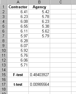
Figure 48. Excel Results for Data from Example Problem 1
The test that is conducted by Excel is a one-sided F-test. The value that is displayed in cell B15 is the probability of getting an F-value as large as the one for these data sets if the two data sets have the same variance. In other words, the lower the probability value returned by this function, the less likely it is that the two sets of data have the same variance. For example, if the level of significance for the test were selected as 0.05, for a one-tailed test you would reject the assumption of equal variances whenever the probability value that is returned by the function is less than 0.05.
To compare the results of function FTEST with the critical values in table 35, which is based on a two-sided F-test and a = 0.01 therefore, you would reject the assumption of equal variances whenever the Excel FTEST function returned a probability value less than 0.005. Figure 48 shows that for the example data a probability value of 0.484 is returned by the FTEST function. Therefore, the conclusion would be to assume that the variances are equal.
Once the results of the F-test are known, the t-test can then be conducted using the Excel function
TTEST(array1,array2,tails,type)
| Where: | array1 is the array representing one set of data. |
| array2 is the array representing the other set of data. | |
| tails is either 1 for a one-sided test or 2 for a two-sided test. | |
| type is 1 for a paired t-test, 2 for an equal variance t-test, and 3
for an unequal variance t-test. |
For the example in figure 48, the contractor data are in array1, and it is input as A2:A13, while the agency data are in array2 and it is input as B2:B7. Since a two-tailed is desired, tails is input as 2, and, since from the F-test the variances were assumed to be equal, type is input as 2. The function that is entered into cell B17 is therefore =TTEST(A2:A13,B2:B7,2,2). Figure 48 shows that for the example data a probability value of 0.00986 is returned by the TTEST function. Therefore, at the a = 0.01 level of significance, the conclusion would be to assume that the means are not equal since the probability value is less than 0.01.
Similarly, Excel can be used to perform the F-test and t-test on the data sets from Example Problem 2 above. This is illustrated in figure 49.
Figure 49. Excel Results for Data from Example Problem 2
The results in figure 49 (see cell B13) indicate that the variances are assumed to be not equal. This means that the type input for the TTEST function will be 3, for an unequal variance t-test. The tails input will still be 2 for a two-tailed test. The results in figure 49 (see cell B15) indicate that the means are assumed to be equal since the probability in cell B15 is much greater than the level of significance of a = 0.01.
Using Program DATATEST
Another software program that can be used for performing F-test and t-test comparisons is the FHWA Demonstration Project No. 89 program DATATEST. (18) This program demonstrates how simply the F-tests and t-tests can be performed with a personal computer. To illustrate this, the DATATEST program was used to compare the data sets used in the example problems above. To illustrate the use of the program, the input and output screens for these examples are presented in the figures beginning on the next page.
DATATEST Screens for the Data from Example Problem 1
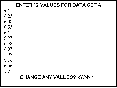
The program first asks for the number of values and then allows the user to input the values for the first set of data.

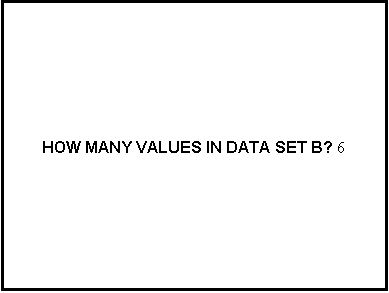
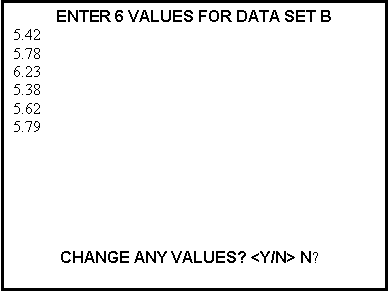
The program then asks for the number of values and then allows the user to input the values for the second set of data.
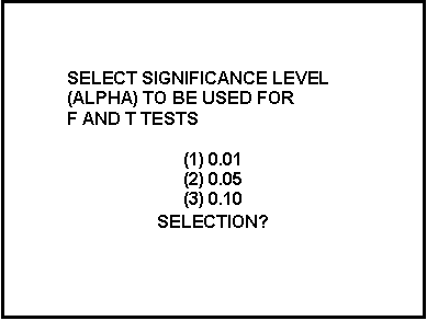
The program then asks the user to select a level of significance, a.

Finally, the program conducts the F-test and then, based on the F-test results, the appropriate form of the t-test, and displays the results.
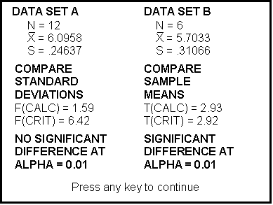
The values obtained by the DATATEST program are consistent with those calculated in Example Problem 1 above. The slight difference in the calculated t- value stems from the number of decimal places that are used in the computer's calculation. The results from the DATATEST program, i.e., the variances not assumed different and the means assumed different, are consistent with those from Example Problem 1.
DATATEST Screens for the Data from Example Problem 2
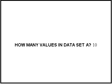
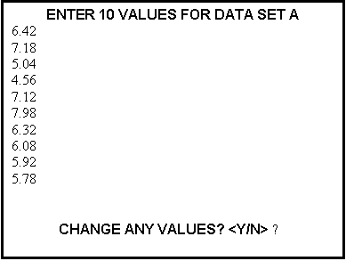
The program first asks for the number of values and then allows the user to input the values for the first set of data.
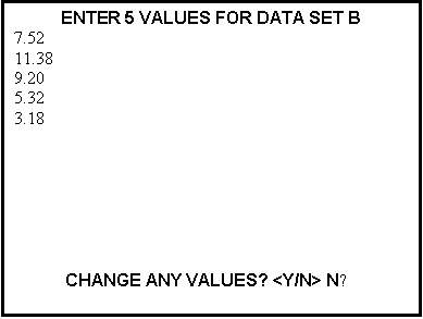
The program then asks for the number of values and then allows the user to input the values for the second set of data.

The program then asks the user to select a level of significance, a.
Finally, the program conducts the F-test and then, based on the F-test results, the appropriate form of the t-test, and displays the results.
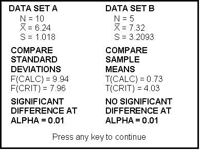
The values obtained by the DATATEST program are consistent with those calculated in Example Problem 2 above. The results from the DATATEST program, i.e., the variances assumed different and the means not assumed different, are consistent with those from Example Problem 2.
| 1 |
2 |
3 |
4 |
5 |
6 |
7 |
8 |
9 |
10 |
11 |
12 |
|
|---|---|---|---|---|---|---|---|---|---|---|---|---|
|
|
16200 |
20000 |
21600 |
22500 |
23100 |
23400 |
23700 |
23900 |
24100 |
24200 |
24300 |
24400 |
2 |
198 |
199 |
199 |
199 |
199 |
199 |
199 |
199 |
199 |
199 |
199 |
199 |
3 |
55.6 |
49.8 |
47.5 |
46.2 |
45.4 |
44.8 |
44.4 |
44.1 |
43.9 |
43.7 |
43.5 |
43.4 |
4 |
31.3 |
26.3 |
24.3 |
23.2 |
22.5 |
22.0 |
21.6 |
21.4 |
21.1 |
21.0 |
20.8 |
20.7 |
5 |
22.8 |
18.3 |
16.5 |
15.6 |
14.9 |
14.5 |
14.2 |
14.0 |
13.8 |
13.6 |
13.5 |
13.4 |
6 |
18.6 |
14.5 |
12.9 |
12.0 |
11.5 |
11.1 |
10.8 |
10.6 |
10.4 |
10.2 |
10.1 |
10.0 |
7 |
16.2 |
12.4 |
10.9 |
10.0 |
9.52 |
9.16 |
8.89 |
8.68 |
8.51 |
8.38 |
8.27 |
8.18 |
8 |
14.7 |
11.0 |
9.60 |
8.81 |
8.30 |
7.95 |
7.69 |
7.50 |
7.34 |
7.21 |
7.10 |
7.01 |
9 |
13.6 |
10.1 |
8.72 |
7.96 |
7.47 |
7.13 |
6.88 |
6.69 |
6.54 |
6.42 |
6.31 |
6.23 |
10 |
12.8 |
9.43 |
8.08 |
7.34 |
6.87 |
6.54 |
6.30 |
6.12 |
5.97 |
5.85 |
5.75 |
5.66 |
11 |
12.2 |
8.91 |
7.60 |
6.88 |
6.42 |
6.10 |
5.86 |
5.68 |
5.54 |
5.42 |
5.32 |
5.24 |
12 |
11.8 |
8.51 |
7.23 |
6.52 |
6.07 |
5.76 |
5.52 |
5.35 |
5.20 |
5.09 |
4.99 |
4.91 |
15 |
10.8 |
7.70 |
6.48 |
5.80 |
5.37 |
5.07 |
4.85 |
4.67 |
4.54 |
4.42 |
4.33 |
4.25 |
20 |
9.94 |
6.99 |
5.82 |
5.17 |
4.76 |
4.47 |
4.26 |
4.09 |
3.96 |
3.85 |
3.76 |
3.68 |
24 |
9.55 |
6.66 |
5.52 |
4.89 |
4.49 |
4.20 |
3.99 |
3.83 |
3.69 |
3.59 |
3.50 |
3.42 |
30 |
9.18 |
6.35 |
5.24 |
4.62 |
4.23 |
3.95 |
3.74 |
3.58 |
3.45 |
3.34 |
3.25 |
3.18 |
40 |
8.83 |
6.07 |
4.98 |
4.37 |
3.99 |
3.71 |
3.51 |
3.35 |
3.22 |
3.12 |
3.03 |
2.95 |
60 |
8.49 |
5.80 |
4.73 |
4.14 |
3.76 |
3.49 |
3.29 |
3.13 |
3.01 |
2.90 |
2.82 |
2.74 |
120 |
8.18 |
5.54 |
4.50 |
3.92 |
3.55 |
3.28 |
3.09 |
2.93 |
2.81 |
2.71 |
2.62 |
2.54 |
7.88 |
5.30 |
4.28 |
3.72 |
3.35 |
3.09 |
2.90 |
2.74 |
2.62 |
2.52 |
2.43 |
2.36 |
1 NOTE: This is for a two-tailed test with the null and alternate hypotheses shown below:
F-17 |


Table 35. Critical Values, F crit , for the F -test for a Level of Significance, = 0.01 1 (continued) degrees of freedom for numerator
|
15 |
20 |
24 |
30 |
40 |
50 |
60 |
100 |
120 |
200 |
500 |
|
1 |
24600 |
24800 |
24900 |
25000 |
25100 |
25200 |
25300 |
25300 |
25400 |
25400 |
25400 |
25500 |
2 |
199 |
199 |
199 |
199 |
199 |
199 |
199 |
199 |
199 |
199 |
199 |
200 |
3 |
43.1 |
42.8 |
42.6 |
42.5 |
42.3 |
42.2 |
42.1 |
42.0 |
42.0 |
41.9 |
41.9 |
41.8 |
4 |
20.4 |
20.2 |
20.0 |
19.9 |
19.8 |
19.7 |
19.6 |
19.5 |
19.5 |
19.4 |
19.4 |
19.3 |
5 |
13.1 |
12.9 |
12.8 |
12.7 |
12.5 |
12.5 |
12.4 |
12.3 |
12.3 |
12.2 |
12.2 |
12.1 |
6 |
9.81 |
9.59 |
9.47 |
9.36 |
9.24 |
9.17 |
9.12 |
9.03 |
9.00 |
8.95 |
8.91 |
8.88 |
7 |
7.97 |
7.75 |
7.65 |
7.53 |
7.42 |
7.35 |
7.31 |
7.22 |
7.19 |
7.15 |
7.10 |
7.08 |
8 |
6.81 |
6.61 |
6.50 |
6.40 |
6.29 |
6.22 |
6.18 |
6.09 |
6.06 |
6.02 |
5.98 |
5.95 |
9 |
6.03 |
5.83 |
5.73 |
5.62 |
5.52 |
5.45 |
5.41 |
5.32 |
5.30 |
5.26 |
5.21 |
5.19 |
10 |
5.47 |
5.27 |
5.17 |
5.07 |
4.97 |
4.90 |
4.86 |
4.77 |
4.75 |
4.71 |
4.67 |
4.64 |
F-18 |
11 |
5.05 |
4.86 |
4.76 |
4.65 |
4.55 |
4.49 |
4.45 |
4.36 |
4.34 |
4.29 |
4.25 |
4.23 |
12 |
4.72 |
4.53 |
4.43 |
4.33 |
4.23 |
4.17 |
4.12 |
4.04 |
4.01 |
3.97 |
3.93 |
3.90 |
15 |
4.07 |
3.88 |
3.79 |
3.69 |
3.59 |
3.52 |
3.48 |
3.39 |
3.37 |
3.33 |
3.29 |
3.26 |
20 |
3.50 |
3.32 |
3.22 |
3.12 |
3.02 |
2.96 |
2.92 |
2.83 |
2.81 |
2.76 |
2.72 |
2.69 |
24 |
3.25 |
3.06 |
2.97 |
2.87 |
2.77 |
2.70 |
2.66 |
2.57 |
2.55 |
2.50 |
2.46 |
2.43 |
30 |
3.01 |
2.82 |
2.73 |
2.63 |
2.52 |
2.46 |
2.42 |
2.32 |
2.30 |
2.25 |
2.21 |
2.18 |
40 |
2.78 |
2.60 |
2.50 |
2.40 |
2.30 |
2.23 |
2.18 |
2.09 |
2.06 |
2.01 |
1.96 |
1.93 |
60 |
2.57 |
2.39 |
2.29 |
2.19 |
2.08 |
2.01 |
1.96 |
1.86 |
1.83 |
1.78 |
1.73 |
1.69 |
120 |
2.37 |
2.19 |
2.09 |
1.98 |
1.87 |
1.80 |
1.75 |
1.64 |
1.61 |
1.54 |
1.48 |
1.43 |
2.19 |
2.00 |
1.90 |
1.79 |
1.67 |
1.59 |
1.53 |
1.40 |
1.36 |
1.28 |
1.17 |
1.00 |
1 NOTE: This is for a two-tailed test with the null and alternate hypotheses shown below:


Table 36. Critical Values,t crit , for the t-test 1
| Degrees of Freedom |
= 0.01 |
= 0.05 |
= 0.10 |
|---|---|---|---|
1 |
63.657 |
12.706 |
6.314 |
2 |
9.925 |
4.303 |
2.920 |
3 |
5.841 |
3.182 |
2.353 |
4 |
4.604 |
2.776 |
2.132 |
5 |
4.032 |
2.571 |
2.015 |
6 |
3.707 |
2.447 |
1.943 |
7 |
3.499 |
2.365 |
1.895 |
8 |
3.355 |
2.306 |
1.860 |
9 |
3.250 |
2.262 |
1.833 |
10 |
3.169 |
2.228 |
1.812 |
11 |
3.106 |
2.201 |
1.796 |
12 |
3.055 |
2.179 |
1.782 |
13 |
3.012 |
2.160 |
1.771 |
14 |
2.977 |
2.145 |
1.761 |
15 |
2.947 |
2.131 |
1.753 |
16 |
2.921 |
2.120 |
1.746 |
17 |
2.898 |
2.110 |
1.740 |
18 |
2.878 |
2.101 |
1.734 |
19 |
2.861 |
2.093 |
1.729 |
20 |
2.845 |
2.086 |
1.725 |
21 |
2.831 |
2.080 |
1.721 |
22 |
2.819 |
2.074 |
1.717 |
23 |
2.807 |
2.069 |
1.714 |
24 |
2.797 |
2.064 |
1.711 |
25 |
2.787 |
2.060 |
1.708 |
26 |
2.779 |
2.056 |
1.706 |
27 |
2.771 |
2.052 |
1.703 |
28 |
2.763 |
2.048 |
1.701 |
29 |
2.756 |
2.045 |
1.699 |
30 |
2.750 |
2.042 |
1.697 |
40 |
2.704 |
2.021 |
1.684 |
60 |
2.660 |
2.000 |
1.671 |
120 |
2.617 |
1.980 |
1.658 |
2.576 |
1.960 |
1.645 |
1 NOTE: This is for a two-tailed test with the null and alternate hypotheses shown below:

