U.S. Department of Transportation
Federal Highway Administration
1200 New Jersey Avenue, SE
Washington, DC 20590
202-366-4000
Federal Highway Administration Research and Technology
Coordinating, Developing, and Delivering Highway Transportation Innovations
 |
| This report is an archived publication and may contain dated technical, contact, and link information |
|
Publication Number: FHWA-RD-02-095 |
Previous | Table of Contents | Next
As discussed in chapter 5, verification testing can be of two types: test method verification testing that is done on split samples, or process verification testing that is done on independent samples. The procedures are different for each of these types of verification testing.
In chapter 5, two methods were considered for test method verification of split samples: the D2S method, which compares the contractor and agency results from a single split sample, and the paired t—test, which compares contractor and agency results from a number of split samples. OC curves, which plot the probability of detecting a difference versus the actual difference between the two populations, can be developed for either of these methods.
In the D2S method, a test is performed on a single split sample to compare agency and contractor test results. If we assume both of these samples are from normally distributed subpopulations, then we can calculate the variance of the difference and use it to calculate two standard deviation, or approximately 95 percent, limits for the sample difference quantity. Suppose the agency subpopulation has a variance ![]() and the contractor subpopulation has a variance
and the contractor subpopulation has a variance ![]() . Since the variance of the difference in two random variables is the sum of the variances, the variance of the difference in an agency observation and a contractor observation is
. Since the variance of the difference in two random variables is the sum of the variances, the variance of the difference in an agency observation and a contractor observation is ![]() . The D2S limits are based on the test standard deviation provided. Let us call this test standard deviation σtest. Under an assumption that
. The D2S limits are based on the test standard deviation provided. Let us call this test standard deviation σtest. Under an assumption that ![]() , this variance of a difference becomes
, this variance of a difference becomes ![]() . The D2S limits are set as two times the standard deviation (i.e., approximately 95 percent limits) of the test differences. This therefore sets that the D2S limits at
. The D2S limits are set as two times the standard deviation (i.e., approximately 95 percent limits) of the test differences. This therefore sets that the D2S limits at ![]() , which is
, which is ![]() , or ±2.8284 σtest. Without loss of generality, we can assume σtest = 1, along with assumption of a mean difference of 0, and use the standard normal distribution with region between -2.8284 and +2.8284 as acceptance region for the difference in an agency test result and a contractor test result. With these two limits fixed, we can calculate power of this decision-making process relative to various true differences in the underlying subpopulation means and/or various ratios of the true underlying subpopulation standard deviations.
, or ±2.8284 σtest. Without loss of generality, we can assume σtest = 1, along with assumption of a mean difference of 0, and use the standard normal distribution with region between -2.8284 and +2.8284 as acceptance region for the difference in an agency test result and a contractor test result. With these two limits fixed, we can calculate power of this decision-making process relative to various true differences in the underlying subpopulation means and/or various ratios of the true underlying subpopulation standard deviations.
These power values can conveniently be displayed as a three-dimensional surface. If we vary the mean difference along the first axis and the standard deviation ratio along a second axis, we can show power on the vertical axis. The agency subpopulation, the contractor subpopulation, or both, could have standard deviations smaller, about the same, or larger than the supplied σtest value. Each of these cases is considered in the technical report for this project.[17] For simplicity, herein we will consider only the case where one of the two subpopulations has standard deviation equal to the supplied σtest. Figure 50 shows the OC curves for this case. Power values are shown where the ratio of the larger of agency or contractor standard deviation to the smaller of agency or contractor standard deviation is varied over the values 0, 1, 2, 3, 4, and 5. The mean difference given along the horizontal axis (values 0, 1, 2, 3) represents the difference in agency and contractor subpopulation means expressed as multiples of σtest.
As can be seen in the figure, even when the ratio of the contractor and agency standard deviations is 5 and the difference between the contractor and agency means is 3 times the value for σtest, there is less than a 70 percent chance of detecting the difference based on the results from a single split sample.
As is the case with any method based on a sample of size one, the D2S method does not have much power to detect differences between the contractor and agency populations. The appeal of the D2S method lies in its simplicity rather than its power.
| Prob. Of Detecting a Difference, % |  |
Std. Dev. Ratio |
| Mean Difference, in σtest Units | ||
Figure 50. OC Surface for the D2S Test Method Verification Method (Assuming the smaller σ= σtest) |
||
As noted in chapter 5, for the case in which it is desirable to compare more than one pair of split sample test results, the t—test for paired measurements can be used. But the question arises, how many pairs of test results should be used? This is where an OC curve is helpful. The OC curve, for a given level of α, plots on the vertical axis either the probability of not detecting, β, or detecting, 1 - β, a difference between two populations. The standardized difference between the two population means is plotted on the horizontal axis.
For a t—test for paired measurements, the standardized difference, d, is measured as:
![]()
| where: | = | the true absolute difference between the mean of the contractor's test result population (which is unknown) and the mean of the agency's test result population (which is unknown). | |
| σd | = | the standard deviation of the true population of signed differences between the paired tests (which is unknown). |
The OC curves are developed for a given level of significance, α. It is evident from the OC curves that for any probability of not detecting a difference, β, (value on the vertical axis), the required n will increase as the difference, d, decreases (value on the horizontal axis). In some cases the desired β or d may require prohibitively large sample sizes. In that case a compromise must be made between the discriminating power desired, the cost of the amount of testing required, and the risk of claiming a difference when none exists.
OC curves for paired t—tests for α values of 0.05 and 0.01 appear in figures 51 and 52, respectively.
To use these OC curves the true standard deviation of the signed differences, σd, is assumed to be known, (or approximated based on published literature). After experience is gained with the process, σd can be more accurately defined and a better idea of the required number of tests determined.
Example 1. The number of pairs of split sample tests for verification of laboratory-compacted air voids using the Superpave Gyratory Compactor (SGC) is desired. The probability of not detecting a difference, β, is chosen as 20 percent or 0.20. (Some OC curves use 1 - β, known as the power of the test, on the vertical axis, but the only difference is the scale change, with 1 - β, in this case, being 80 percent). Assume that the absolute difference between μc and μa should not be greater than 1.25 percent, that the standard deviation using the SGC is 0.5 percent, and that α is selected as 0.01. This produces a d value of 1.25 percent/0.5 percent = 2.5. Reading this value on the horizontal axis and a β of 0.20 on the vertical axis in figure 52 shows that about 5 paired split-sample tests are necessary for the comparison.
 |
 |
| Standardized Difference, d | |
Figure 51. OC Curves for a Two—Sided t—Test (α = 0.05 ) |
|
| (Source: Experimental Statistics, by M. G. Natrella, National Bureau of Standards Handbook 91, 1963) | |
|
 |
| Standardized Difference, d | |
Figure 52. OC Curves for a Two-Sided t—Test (α = 0.01) |
|
| (Source: Experimental Statistics, by M. G. Natrella, National Bureau of Standards Handbook 91, 1963) | |
In chapter 5, two methods were considered for process verification using independently obtained samples: the F—test and t—test method, which compares the variances and means of sets of contractor and agency test results, and the single agency test method, which compares a single agency test result with 5 to 10 contractor test results. OC curves, which plot the probability of not detecting a difference, β, or detecting a difference, the power or 1 - β, versus the actual difference between the two populations, can be developed for either of these methods.
One approach for comparing the contractor's test results with the agency's test results is to use the F—test and t—test comparisons of characteristics of the two data sets. To compare two populations that are assumed normally distributed, it is necessary to compare their means and their variabilities. An F—test is used to assess the size of the ratio of the variances, and a t—test is used to assess the degree of difference in the means. A question that needs to be answered is what power do these statistical tests have, when used with small to moderate size samples, to declare various differences in means and variances to be statistically significant differences. Some OC curves and examples of their use in power analysis follow.
F—test for Variances——Equal Sample Sizes. Suppose we have two sets of measurements assumed to come from normally distributed populations and wish to conduct a test to see if they come from populations that have the same variances, i.e., ![]() . Further suppose we select a level of significance of α = .05, meaning we are allowing up to 5 percent chance of incorrectly deciding the variances are different when they really are the same. If we assume these two samples are
. Further suppose we select a level of significance of α = .05, meaning we are allowing up to 5 percent chance of incorrectly deciding the variances are different when they really are the same. If we assume these two samples are
x1, x2, …, xnx, and y1, y2 , …, yny,
calculate sample variances ![]() and
and ![]() , and construct
, and construct
![]() ,
,
we would accept Ho : ![]() for values of F in the interval
for values of F in the interval
![]() .
.
For this two-sided or two-tailed test, figure 53 shows the probability we have accepted the two samples as coming from populations with the same variabilities. This probability is usually referred to as β, and the power of the test as 1 - β. Notice the horizontal axis is the quantity λ, where ![]() , the true standard deviation ratio. So for λ = 1, where the hypothesis of equal variance should certainly be accepted, it is accepted with probability 0.95, reduced from 1.0 only by the magnitude of our selected type I error risk, α. One major limiting factor for the use of figure 53 is the restriction that nx = ny = n.
, the true standard deviation ratio. So for λ = 1, where the hypothesis of equal variance should certainly be accepted, it is accepted with probability 0.95, reduced from 1.0 only by the magnitude of our selected type I error risk, α. One major limiting factor for the use of figure 53 is the restriction that nx = ny = n.
Example 2. Suppose we have nx = 6 contractor tests and ny = 6 agency tests, conduct an α = 0.05 level test, and accept that these two sets of tests represent populations with equal variances. What power did our test have to discern if the populations from which these two sets of tests came were really rather different in variabilities? Suppose the true population standard deviation of the contractor tests (σx) was twice as large as that of the agency tests (σy), giving λ = 2. If we enter figure 53 with λ = 2 and nx = ny = 6, we find that β ≈ 0.74, or the power, 1 - β, is about 0.26. This tells us that with samples of nx = 6 and ny = 6, we only have 26 percent chance of detecting a standard deviation ratio of 2 (and correspondingly a four-fold difference in variance) as being different.
Example 3. Suppose we are not at all comfortable with the power of 0.26 in Example 1, and so subsequently we increase the number of tests used. Suppose we now have nx = 20 and ny = 20. If we again consider λ = 2, we can determine from figure 53 the power of detecting these sets of tests as coming from populations with unequal variances to be over 0.8, approximately 82 percent to 83 percent. If we proceed to conduct our F-test with these two samples, and conclude the underlying variances are equal, we certainly feel much more comfortable with our conclusions.
Figure 54 gives the appropriate OC curves to use if we choose to conduct an α = 0.01 level test. Again we see for equal variances σx2 and σy2, giving λ = 1, that β = 0.99, reduced from 1.0 only by the size of α.
F—test for Variances—Unequal Sample Sizes. Up to now the discussions and OC curves presented have been limited to the case when the two sample sizes are equal. Calculation routines were developed for this project for calculation of power for this test for any combination of sample sizes nx and ny. There are obviously an infinite number of possible combinations for nx and ny. So, it is not possible to present OC curves for every possibility. However, three sets of tables are provided herein which provide a subset of power calculations using some sample sizes that are of potential interest for comparing contractor and agency samples. These power calculations are presented in table form since there are too many variables to present in a single chart, and the data can be presented in a more compact form in tables than in a long series of charts. Table 37 gives power values for all combinations of sample sizes from 3 to 10, with the ratio of the two subpopulation standard deviations being 1, 2, 3, 4, and 5. Table 38 gives power values for the same sample sizes, but with the standard deviation ratios being 0.0, 0.2, 0.4, 0.6, 0.8, and 1.0. Table 39 gives power values for all combinations for sample sizes of 5, 10, 15, 20, 25, 30, 40, 50, 60, 70, 80, 90, and 100, with the standard deviation ratio being 1, 2, or 3. An example below illustrates the use of the first of these tables to reference power for a hypothetical test.
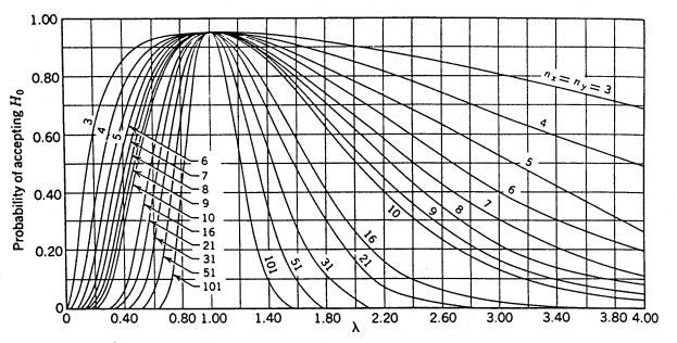 |
| Figure 53. OC Curves for the Two—Sided F—Test for Level of Significance α = 0.05 (Source: Engineering Statistics by A. H. Bowker and G. J. Lieberman.) |
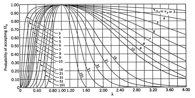 |
| Figure 54. OC Curves for the Two—Sided F—Test for Level of Significance α = 0.01 (Source: Engineering Statistics by A. H. Bowker and G. J. Lieberman.) |
Table 37. F—test Power Values for n = 3 to 10 and s—ratio, λ = 1 to 5
|
|
|
Table 37. F-test Power Values for n = 3 to 10 and s-ratio, λ = 1 to 5 (cont.)
|
|
|
Table 37. F-test Power Values for n = 3 to 10 and s-ratio, λ = 1 to 5 (cont.)
| λ | ny | nx | Power |
|---|---|---|---|
| 5 | 7 | 3 | 0.75893 |
| 4 | 0.84940 | ||
| 5 | 0.90024 | ||
| 6 | 0.93086 | ||
| 7 | 0.95030 | ||
| 8 | 0.96318 | ||
| 9 | 0.97201 | ||
| 10 | 0.97824 | ||
| 8 | 3 | 0.77800 | |
| 4 | 0.86909 | ||
| 5 | 0.91845 | ||
| 6 | 0.94695 | ||
| 7 | 0.96423 | ||
| 8 | 0.97513 | ||
| 9 | 0.98225 | ||
| 10 | 0.98704 | ||
| 9 | 3 | 0.79133 | |
| 4 | 0.88238 | ||
| 5 | 0.93024 | ||
| 6 | 0.95690 | ||
| 7 | 0.97244 | ||
| 8 | 0.98184 | ||
| 9 | 0.98772 | ||
| 10 | 0.99150 | ||
| 10 | 3 | 0.80115 | |
| 4 | 0.89188 | ||
| 5 | 0.93838 | ||
| 6 | 0.96351 | ||
| 7 | 0.97767 | ||
| 8 | 0.98594 | ||
| 9 | 0.99092 | ||
| 10 | 0.99400 |
Table 38. F-test Power Values for n = 3 to 10 and s-ratio, λ = 0.0 to 1.0
|
|
|
Table 38. F-test Power Values for n = 3 to 10 and s-ratio, λ = 0.0 to 1.0 (cont.)
|
|
|
Table 38. F-test Power Values for n = 3 to 10 and s-ratio, λ = 0.0 to 1.0 (cont.)
|
|
Table 39. F-test Power Values for n = 5 to 100 and s-ratio, λ = 1 to 3
|
|
|
Table 39. F-test Power Values for n = 5 to 100 and s-ratio, λ = 1 to 3 (cont.)
|
|
|
Table 39. F-test Power Values for n = 5 to 100 and s-ratio, λ = 1 to 3 (cont.)
|
|
|
Table 39. F-test Power Values for n = 5 to 100 and s-ratio, λ = 1 to 3 (cont.)
|
|
|
Table 39. F-test Power Values for n = 5 to 100 and s-ratio, λ = 1 to 3 (cont.)
| λ | ny | nx | Power |
|---|---|---|---|
| 3 | 80 | 5 | 0.85871 |
| 10 | 0.98476 | ||
| 15 | 0.99831 | ||
| 20 | 0.99980 | ||
| 25 | 0.99998 | ||
| 30 | 1.00000 | ||
| 40 | 1.00000 | ||
| 50 | 1.00000 | ||
| 60 | 1.00000 | ||
| 70 | 1.00000 | ||
| 80 | 1.00000 | ||
| 90 | 1.00000 | ||
| 100 | 1.00000 | ||
| 90 | 5 | 0.86026 | |
| 10 | 0.98537 | ||
| 15 | 0.99844 | ||
| 20 | 0.99983 | ||
| 25 | 0.99998 | ||
| 30 | 1.00000 | ||
| 40 | 1.00000 | ||
| 50 | 1.00000 | ||
| 60 | 1.00000 | ||
| 70 | 1.00000 | ||
| 80 | 1.00000 | ||
| 90 | 1.00000 | ||
| 100 | 1.00000 | ||
| 100 | 5 | 0.86150 | |
| 10 | 0.98584 | ||
| 15 | 0.99855 | ||
| 20 | 0.99985 | ||
| 25 | 0.99998 | ||
| 30 | 1.00000 | ||
| 40 | 1.00000 | ||
| 50 | 1.00000 | ||
| 60 | 1.00000 | ||
| 70 | 1.00000 | ||
| 80 | 1.00000 | ||
| 90 | 1.00000 | ||
| 100 | 1.00000 |
Example 4. Suppose we have nx = 10 contractor tests and ny = 6 agency tests, conduct an α = 0.05 level test, and accept that these two tests represent populations with equal variances. What power did our test have to discern if the populations from which these two sets of tests came were really rather different in variabilities? Suppose the true population standard deviation of the contractor's test population (σx) was twice as large as that of the agency's test population (σy), giving a standard deviation ratio value, λ = 2. If we enter table 37 with λ = 2, nx = 10, and ny = 6, we find the power to be 0.29722. This tells us that with samples of nx = 10 and ny = 6, we have slightly less than a 30 percent chance of detecting a standard deviation ratio of 2 (and correspondingly a four-fold difference in variances) as being different.
t—test for Means. Suppose we have two sets of measurements, assumed to be from normally distributed populations, and wish to conduct a two-sided or two-tailed test to see if these populations have equal means, i.e., μx = μy. Suppose we assume these two samples are from populations with unknown, but equal, variances. If these two samples are x1, x2, …, xnx with sample mean ![]() and sample variance
and sample variance ![]() , and y1, y2, …, yny with sample mean
, and y1, y2, …, yny with sample mean ![]() and sample variance
and sample variance ![]() , we can calculate
, we can calculate
and accept Ho: μx = μy for values of t in the interval ![]() .
.
For this test, figure 51 or 52, depending upon the α value, shows the probability we have accepted the two samples as coming from populations with the same means. The horizontal axis scale is
![]()
where σ - σx = σy is the true common population standard deviation. We access the OC curves in figure 51 and 52 with a value for d of d* and a value for n of n' where
![]()
and
![]()
Example 5. Suppose we have nx = 8 contractor tests and ny = 8 agency tests, conduct an α = 0.05 level test, and accept that these two sets of tests represent populations with equal means. What power did our test really have to discern if the populations from which these two sets of tests came had different means? Suppose we consider a difference in these population means of 2 or more standard deviations as a noteworthy difference that we would like to detect with high probability. This would indicate that we are interested in d = 2. Calculating
![]()
and
We find from figure 51 that β ≈ 0.05 so that our power of detecting a mean difference of 2 or more σ would be approximately 95 percent.
Example 6. Suppose we consider an application where we still have a total of 16 tests, but with nx = 12 contractor tests and ny = 4 agency tests. Suppose that we are again interested in t—test performance in detecting a means difference of 2 standard deviations. Again
![]()
but now
We find from figure 51 that β ≈ 0.12 indicating a power of approximately 88 percent of detecting a mean difference of 2 or more standard deviations.
Figure 52 gives the appropriate OC curves for our use in conducting an α = 0.01 level test on means. This figure is accessed in the same manner as described above for figure 51.
This procedure involves comparing the mean of 5 to 10 contractor tests with a single agency test result. The two are considered to be similar if the agency test is within an allowable interval on either side of the mean of the contractor's test results. The allowable interval is determined by multiplying the sample range of the contractor's test results by a factor that depends on the number of contractor test results. The equations for computing the allowable intervals are shown in table 40.
This comparison method is adapted from an approach for calculating the confidence interval for estimating a population mean. A confidence interval for a population mean is calculated about a sample mean and defines an interval within which there is a given percent confidence that the true population mean falls. When the variability of the population is unknown, a t-distribution, rather than a normal distribution, is used to calculate the confidence interval for the population mean. The t-distribution is what is used to establish the critical values for the t-statistic that is used in the t—test procedure that was presented above.
When calculating a confidence interval for the population mean, the t-statistic, which is similar in general concept to the Z-statistic of a normal distribution, is used. The t-statistic depends upon the degrees of freedom, defined as n - 1 where n is the number of values used to obtain the sample mean. The confidence interval is defined by:
![]()
The value of t depends upon the number of degrees of freedom and the level of significance chosen for the confidence interval. For example, for a 98 percent confidence interval, the value of t would be the value such that 98 percent of a t-distribution with n - 1 degrees of freedom fell within the mean and ± t standard deviations.
The single agency test approach uses this 98 percent confidence interval to approximate the interval within which a single test result should fall if sampled from a population with mean and standard deviation equal to the sample mean and standard deviation of the contractor's test results. For simplicity, the sample range, R, instead of the sample standard deviation, is used to estimate the population standard deviation. The population standard deviation can be estimated by dividing the sample range by a factor known as d2. Therefore, R ÷ d2 is taken as an estimate of the population standard deviation.
The approach assumes that the population mean is equal to the sample mean of the contractor's tests and that the population standard deviation is equal to the contractor's sample range divided by d2. The interval within which the single agency test result must fall is defined by the interval within which 98 percent of the single test results should fall. The 98 percent confidence interval is calculated based on the t-statistic.
To arrive at the factors in the table for determining the interval around the contractor's test mean within which the agency test must fall, the t-statistic for a 98 percent confidence interval and n - 1 degrees of freedom is multiplied by (R ÷ d2). Since it is a two-sided confidence interval, a 98 percent confidence interval corresponds to the ± t-statistic, t.99, above or below which there is only 1 percent of the t-distribution. The values necessary to develop the interval factors for this comparison method are shown in table 40.
Table 40. Derivation of the Single Agency Test Method Allowable Intervals
| Sample Size, n | Degrees of Freedom, n — 1 |
t—statistic for which there is a 1% chance of being exceeded, t.99 | d2 | Interval |
|---|---|---|---|---|
| 10 | 9 | 2.821 | 3.078 | |
| 9 | 8 | 2.896 | 2.970 | |
| 8 | 7 | 2.998 | 2.847 | |
| 7 | 6 | 3.143 | 2.704 | |
| 6 | 5 | 3.365 | 2.534 | |
| 5 | 4 | 3.747 | 2.326 |
To illustrate the lack of power that this method has to discern differences between populations, the computer program ONETEST was developed as part of FHWA Demonstration Project 89.[18] The ONETEST program assumes that the two sets of data have the same standard deviation value (an assumption that is part of the single test comparison method), and designates in standard deviation units the distance between the true means of the two datasets. The program then determines the probability of detecting the difference for various actual differences between the population means.
ONETEST was used to generate 6,000 comparisons for each of a number of different scenarios, i.e., comparing a single test result to samples of size 10, 9, 8, 7, 6, and 5. In each case, the two populations were assumed to have the same standard deviation, and the difference between the means of the two populations, stated in standard deviation units, Δ = (μ1 - μ2)/σ, varied from 0.0 to 3.0 in increments of 0.5. The results from this analysis are plotted as an OC curve in figure 55.
As can be seen in the OC curve in figure 55, even when the difference between population means was three standard deviations, the percentage of the time this procedure was able to determine a difference in populations ranged from only 58 percent for a sample size of 10 to 34 percent for a sample size of 5.
 |
n = 10 n = 9 n = 8 n = 7 n = 6 n = 5 |
|
Difference in Population Means, Figure 55. OC Curves for the Single Agency Test Method |
||

