U.S. Department of Transportation
Federal Highway Administration
1200 New Jersey Avenue, SE
Washington, DC 20590
202-366-4000
Federal Highway Administration Research and Technology
Coordinating, Developing, and Delivering Highway Transportation Innovations
 |
| This report is an archived publication and may contain dated technical, contact, and link information |
|
Publication Number: FHWA-04-122 Date: February 2005 |
Previous | Table of Contents | Next
In HIPERPAV II (software version 3.0), several changes were made to the software from the previous release of HIPERPAV I (software version 2.X). This user's manual outlines those changes and discusses the new input needed. For information on the theory behind HIPERPAV II, refer to the guidelines (chapters 2 through 5).
In HIPERPAV II, the user can now perform early-age behavior analyses for jointed concrete pavement, evaluate the impacts of early-age factors on JPCP long-term performance, and perform analysis for CRCP (see figure 82).
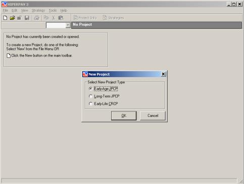
Figure 82. Project type selection screen for HIPERPAV II analysis.
The input screens for these three project types are described below.
After the user selects a project type in the new project window (figure 82), the software creates a strategy with default inputs that the user can modify with the inputs for a specific situation.
There are two primary sections in HIPERPAV II: the project information section discussed below, and strategies section discussed later.
Regardless of the project type, project information is needed for all of the HIPERPAV II analyses. Under the project information screen (figure 83), the user can enter general project information, including the project name, project ID, section name, and beginning and ending stations. A comment box is also provided for any additional information.
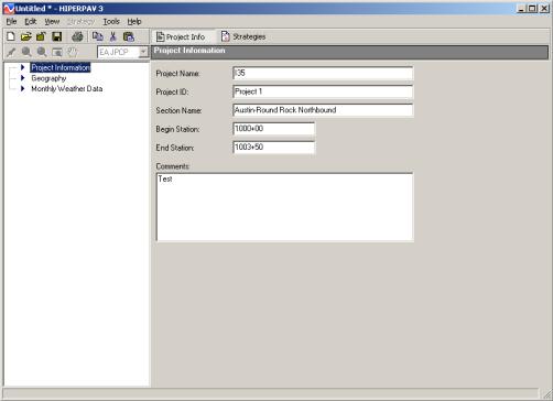
Figure 83. Project information screen for HIPERPAV II analysis.
In the geography screen, the user can select the position within the 50 U.S. States where the project is located (figure 84). Historical weather data from nearby weather stations to the site can be used during the analysis if desired. Climatic information including air temperatures, windspeed, relative humidity, cloudiness, and annual rainfall conditions will be estimated based on this location from the nearest weather stations. Section 7.3.7 provides additional information on selecting the project location.
To navigate the geography screen, five icons are available for use. The user can:
 Magnify the map.
 Decrease magnification of the map.
 Select the location of the project.
 Drag the map.
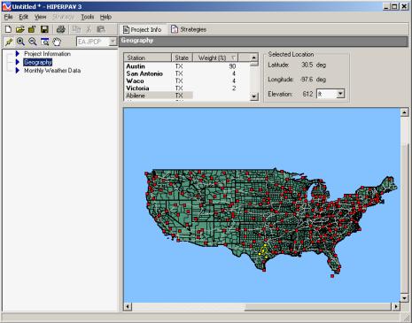
Figure 84. Geography screen for HIPERPAV II analysis.
Monthly rainfall data is used for the long-term analysis only. If the user has more accurate rainfall data, it can be entered in the monthly weather data screen (figure 85).
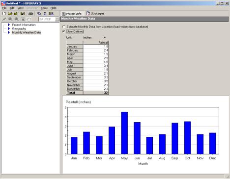
Figure 85. Monthly weather data screen for HIPERPAV II analysis.
After the user selects option 1 in the project type selection screen (figure 82), and the general project information is entered, one or more strategies for that specific location can be created for analysis under the strategies section (figure 86).
The strategies section contains, in tree view, the specific input data required to perform an early-age JPCP analysis under the categories of:
It is possible to have multiple strategies in one project. Each of the strategies can have different design, materials and mix design, construction, and environment inputs.
The strategy toolbar is provided to manipulate strategies. The strategy toolbar includes the following commands:
 Add a strategy
 Copy the currently selected strategy.
 Delete a strategy.
 Validate a strategy to verify that inputs are within allowable ranges.
 Run an analysis for the currently selected strategy.
All the above functions can also be performed by right clicking on the strategy name.
To perform an early-age JPCP analysis, a new strategy must be added. With the strategy created, the strategy information including design, materials and mix design, construction, and environment information can be entered. The screens where this information is entered are listed in a menu format on the left side of the HIPERPAV II screen. As shown on the strategy information screen (figure 86), the user can enter his or her name and chosen reliability level. After the strategy is run, the date of analysis also will appear on this screen. A comment box is available for each strategy.
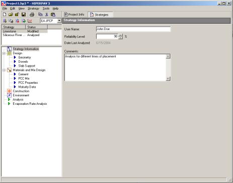
Figure 86. Strategy information screen for HIPERPAV II analysis.
Under the design inputs, the user can enter the pavement design information, including pavement geometry, dowel design, and slab support information.
Under geometry (figure 87), fields to enter the slab thickness, slab width, and transverse joint spacing are provided. For any input in HIPERPAV II, the user can select from several either metric or English units and can convert between unit systems. To convert value, check the convert value box and click on the desired unit.
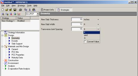
Figure 87. Geometry screen.
A schematic of the geometry input entered in HIPERPAV II is shown in figure 88. The slab width that should be input in HIPERPAV II is the widest spacing between adjacent longitudinal joints. Similarly, the transverse joint spacing in the case of random joint spacings should be the largest spacing between transverse joints (although the user can run each joint spacing as a separate strategy to compare the results).
Figure 88. Schematic of the geometry input in HIPERPAV II.
The dowels design information is entered only if the user wants to evaluate the bearing stresses at the dowels during the early age. The dowel analysis module can assess how dowel bars affect the early-age performance of the joint in jointed concrete pavements (e.g., how the bearing stress of the dowel on the concrete changes as a function of temperature and time will be calculated). If the bearing stress is greater than the concrete's early-age bearing strength, then it is probable that the dowel will loosen in the pavement at a faster rate than if the bearing stress was designed to be less than the concrete's bearing strength. Cyclic loadings, particularly during the early age, commonly cause crushing of the concrete at the dowel interface due to the high stresses at those locations. Voids at the dowel-concrete interface will eventually cause the dowel to provide reduced load transfer efficiency.
If this module is enabled, then the dowel size, Poisson's ratio, and modulus must be input (figure 89). In addition, the 28-day effective modulus of dowel support is required. The modulus of dowel support is defined as "the bearing stress in the concrete mass developing under unit deflection of the bar."(54)Additional information is required on concrete compressive strength under the PCC properties screen if a dowel analysis is to be performed.
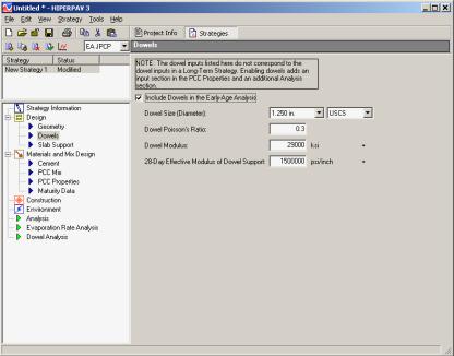
Figure 89. Dowel input screen.
The slab support screen requires information on the material type directly underneath the slab (see figure 90). Options are provided for different subbase types or subgrade conditions (see pulldown menu in figure 91). Additionally, information on the subgrade stiffness in terms of modulus of subgrade reaction (k-value) or subgrade resilient modulus, and subbase thickness and subbase elastic modulus are required.
The k-value may be obtained by: 1) correlations with soil types and other subgrade support tests (i.e., CBR, R-value, etc.); 2) determination of elastic modulus of individual layers (e.g., with the use of deflection testing) and backcalculation methods; or 3) plate load testing methods.
AASHTO T 274 may be used to characterize relatively low stiffness materials such as natural soils, unbound granular materials, stabilized materials, and asphalt concrete. Alternatively, the repeated-load indirect tensile test method ASTM D 4123 may be used to test bound or higher stiffness materials such as stabilized bases and asphalt concrete. The elastic modulus of base materials with a high cement content may be obtained with the ASTM C 469 test method.
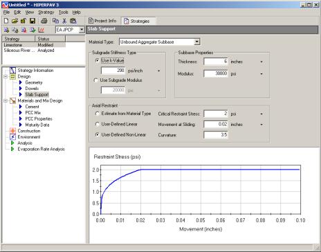
Figure 90. Slab support input screen.
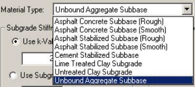
Figure 91. Available subbase types or subgrade conditions.
The axial restraint conditions can be estimated based on the layer directly underneath the slab, or can be user-defined with linear or nonlinear functions that best match the restraint stress-movement curve from field restraint tests. A restraint or pushoff test consists of casting a small slab with an approximate thickness of the projected pavement on top of the same subbase type. A horizontal force is applied on one side of the slab with a hydraulic jack and a load cell is used to measure the applied load. Dial gages are installed at the opposite side to measure the slab movement. The restraint stress is determined from the applied force divided by the area of the test slab. The testing history of restraint stress and slab movement during the pushoff procedure is recorded, and the restraint stress at free sliding is evaluated.(55)
The second input category is materials and mix design. This input category includes the cement, PCC mix, PCC properties, and maturity data inputs.
Under the cement input screen shown in figure 92, the user selects the type of cement either by ASTM cement type classification (pulldown in figure 93), user-defined oxides, or user-defined Bogue compounds. If selected, the user-defined oxides or user-defined Bogue compounds are entered in tabular form.
Blaine fineness can be estimated from the cement type or user-defined if this information is available.
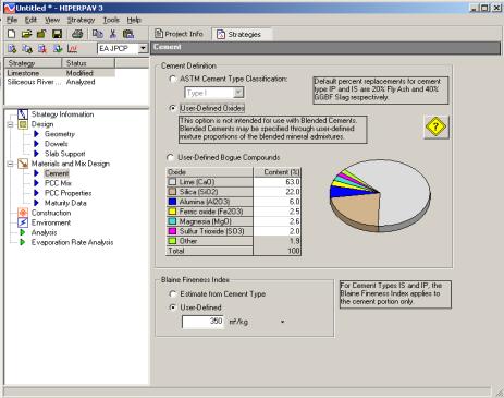
Figure 92. Cement input screen.
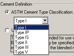
Figure 93. Available cement types in HIPERPAV II.
A help screen that explains the heat of hydration effects of different cementitious materials in HIPERPAV II is available in this screen (see figure 94).
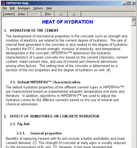
Figure 94. Heat of hydration help screen in HIPERPAV II.
The PCC mix screen is used to enter the mix design related information (figure 95). Under the PCC mix screen, the user selects the type of coarse aggregate used in the mix (see pulldown menu in figure 96), the user can also enter the type of chemical admixtures according to ASTM C 494 (see pulldown in figure 97). Note that Type A and F are not included, because they would not affect the analysis (hover over to see tool tip). If fly ash is used, it is necessary to specify the fly ash class and approximate calcium oxide (lime) content for Class F (see pulldown menu in figure 98). Batch proportions by mass are also entered in this screen.
 Help
icons are provided in several software screens to provide additional guidance on the proper selection of inputs.
Help
icons are provided in several software screens to provide additional guidance on the proper selection of inputs.
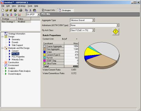
Figure 95. PCC mix input screen.
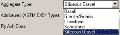
Figure 96. Available coarse aggregate types in HIPERPAV II.
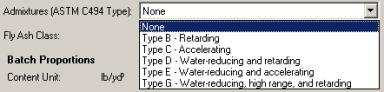
Figure 97. Available admixture types in HIPERPAV II.
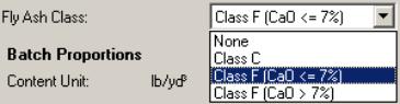
Figure 98. Fly ash class drop-down menu.
The PCC properties screen includes inputs for the 28-day strength, concrete CTE, 28-day modulus, and ultimate drying shrinkage (figure 99).
The 28-day tensile strength is determined through the ASTM C 496 or AASHTO T 198 splitting tensile test. Alternatively, the user can estimate the splitting tensile strength based on relationships with other strength types (see pulldown menu in figure 100). In the equations shown on the screen, "STR" is the PCC 28-day strength type. The splitting tensile strength (STS) is used to predict the formation of cracks in the early-age JPCP. The compressive strength (CS) is used to assess dowel-bearing stresses at early ages with the dowel analysis module. Default conversion values are provided in HIPERPAV II, however, the user is cautioned to develop project specific coefficients based on laboratory testing for the mix in study (see figure 101).
The PCC modulus of elasticity may be determined with ASTM C 469. AASHTO T 160 test procedure at 40 percent relative humidity may be used to determine PCC ultimate drying shrinkage. This test is equivalent to ASTM C 157. The PCC CTE can be entered or estimated by HIPERPAV II based on the coarse aggregate CTE. The latter can be user-defined or estimated based on default values. AASHTO has recently developed a provisional standard that can be used for testing the concrete CTE: TP-60-00, "Standard Test Method for the Coefficient of Thermal Expansion of Hydraulic Cement Concrete."
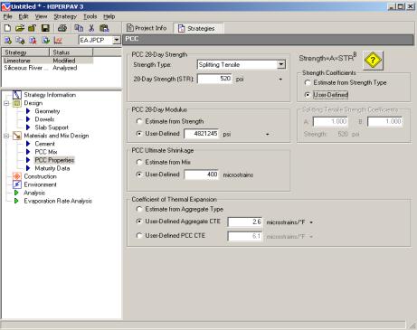
Figure 99. PCC properties screen for early-age JPCP analysis.
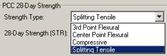
Figure 100. Strength type drop-down menu.
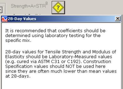
Figure 101. Help icon under PCC properties screen.
The last input under the materials and mix design category is used to enter maturity data, if available. Two methods of maturity are provided: the temperature-time factor with the use of the Nurse-Saul maturity relationships according to ASTM 1074; or the equivalent age method with the use of the Arrhenius relationships. For either method, maturity and strength information are entered in a gridline and automatically plotted on the screen, as shown in figure 102.
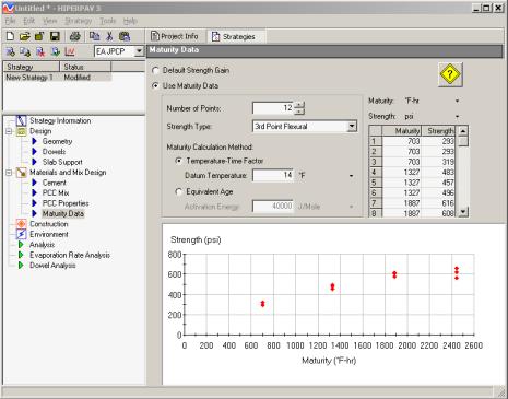
Figure 102. Maturity data input screen.
The third input category corresponds to construction information (figure 103). In this screen, the initial temperatures of the concrete mix and support layer are entered. Information on the curing method used is required, as is the age at which curing is applied. The age when curing is applied is defined as the time elapsed from construction to the time when the slab is covered with membrane curing compounds or polyethylene sheeting. If removable curing methods such as polyethylene sheeting are selected, the age when curing is removed is required. Available curing methods are presented in the drop-down menu for curing method shown in figure 104. A help icon is also available in the curing method inputs, which includes information on the effects of curing type selection.
Information on when joints are cut is also entered in this screen. Three sawcut options are available to the user:
In addition, if a given strength for opening to traffic is required, this information can be entered in the construction inputs screen. Figure 104 shows the strength types that can be entered. Also, as shown in figure 104, a help icon for strength for opening to traffic input is provided. After the analysis is run, the strength for opening to traffic is indicated in the analysis screen (later shown in figure 110) if this strength is achieved within the 72-hour analysis period.
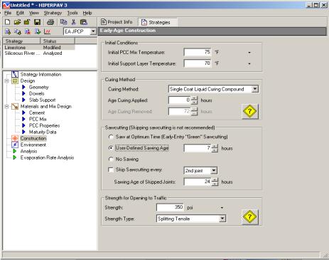
Figure 103. Construction screen.
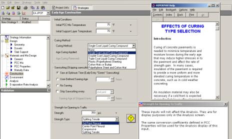
Figure 104. Drop-down menus and help screens under construction inputs.
The last input category corresponds to environment. Under this input category, the user can enter climatic conditions for the 72 hours following construction, as shown in figure 105.
Using the HIPERPAV II environmental database, it is possible to estimate temperature, windspeed, humidity, and cloud cover for any location selected in the geography screen (figure 84). Or, if the user wishes, specific hourly weather data can be entered in the gridlines provided. The information displayed in this screen corresponds to the climatic input selected in the data to display drop-down menu shown in figure 106.
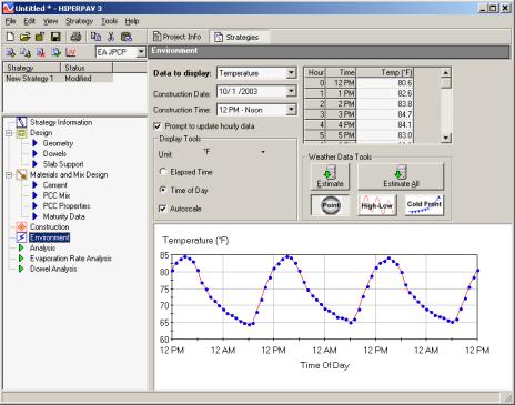
Figure 105. Environment screen.
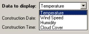
Figure 106. Drop-down menu for selection of climatic input screen to display.
If the construction date or time are changed, it is important that all of the temperature, windspeed, humidity, and cloud cover inputs be estimated again using the "estimate" or "estimate all" icons to match the selected point in time based on the geographic location selected. "Estimate" updates only the data displayed on the current screen. "Estimate all" updates all the weather data under temperature, windspeed, humidity, and cloud cover. The "prompt to update hourly data" checkbox can be unchecked to automatically update weather data as a function of changes in construction time or construction date. Otherwise, a prompt asking to update weather data will appear whenever a change in construction time or date is made.
The user also has the options to:
Options for plotting weather data in terms of elapsed time from construction or for time of day are provided. In addition, an autoscale feature can be selected to cover a wider or narrower weather data range.
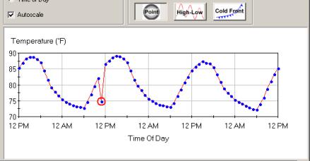
Figure 107. Time-temperature distribution modified with the point feature.
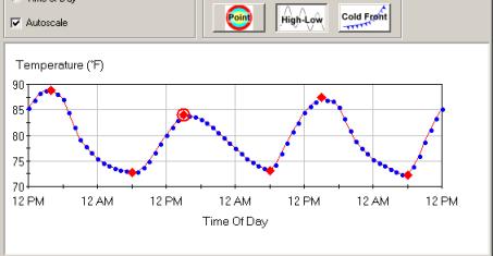
Figure 108. Time-temperature distribution modified with the high-low feature.
Figure 109. Time-temperature distribution modified subjected to a cold front.
With the input assigned, the user should save the inputs before performing an early-age JPCP analysis.
After the analysis is run, a window appears showing the analysis status, and the stresses at the top and at the bottom of the slab are plotted along with the development of the tensile strength in the concrete, as shown in figure 110.
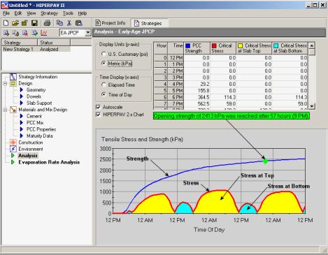
Figure 110. Analysis screen for early-age JPCP.
The numerical stress and strength values also are presented. The critical stress is the largest tensile stress, whether it is at the top or at the bottom of the slab. The numerical value of tensile stress and strength can also be obtained by hovering the mouse over the point of interest. The point in time when the strength for opening to traffic is reached is indicated here in green (highlighted with an arrow and circle for clarity).
Also, because more than one strategy can be analyzed with HIPERPAV II, comparisons can be made between the analysis results more easily. It is possible to toggle between the analysis screens by selecting one strategy and then the other one (for this, the user must have at least two strategies previously analyzed for comparison and toggle between them).
HIPERPAV executes a series of powerful algorithms that calculate the PCC pavement stress and strength development continuously for the first 72 hours following placement. The user is presented with a graphical screen, which plots the results of the analysis as they are computed in real time. The user can observe the trend of the strength and stress development and assess the behavior of the pavement based on the specific user inputs. Following processing, HIPERPAV will then identify possible problem areas and inform the user that the potential for early-age damage is present with the given set of inputs.
Figure 110 shows an output screen from a typical run that demonstrates mix design, pavement design, and construction during PCC pavement placement that lead to a high probability of good performance. The strength curve is the top curve, which remains above the stress curve at all times during the first 72 hours. Note the cyclical manner in which the critical stress occurs. Peaks in the stress curve occur at critical periods when either the axial stresses are dominant or when curling stresses are dominant; the former is in the early morning hours, and the latter is just after midday. In this scenario, the probability for PCC pavement distress (random transverse cracking) is low, because the stress does not exceed the strength during the first 72 hours after placement.
Figure 111 shows an output screen from a typical run where the combination of mix design, pavement design, construction, and the conditions during placement are such that the probability of a poorly performing PCCP is significant. The inputs for this particular run differ from that in figure 110 only by the minimum ambient temperature. A lower value of minimum ambient temperature was used for the scenario presented in figure 111, thus resulting in a thermal shock, which can lead to premature cracking.
The objective of the HIPERPAV guidelines and the accompanying computer software module is to minimize damage to the PCCP during early ages (first 72 hours after placement). By following the general recommendations made in previous chapters of this document in conjunction with the software described in this manual, the chances for achieving this objective are increased substantially.
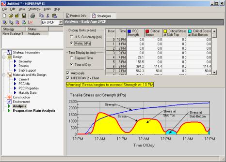
Figure 111. HIPERPAV II early-age analysis showing poor performance.
An analysis screen also is provided for evaporation rate (figure 112). The effect of curing methods is not considered on the evaporation rate analysis. The evaporation rate analysis is a function of the windspeed, relative humidity, air temperature, and HIPERPAV II predicted concrete temperatures. The predicted evaporation rate is presented in both graphic and tabular form in this screen.
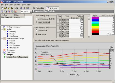
Figure 112. Evaporation rate analysis for early-age JPCP analysis.
The dowel analysis screen compares the concrete bearing strength to the bearing stress generated in proximity to the dowels due to slab curling as shown in figure 113. Because slabs in the field may show different curling conditions from one slab to the other, two scenarios are considered: 1) two slabs with similar curling conditions (curl-curl stress); and 2) one slab flat and the adjacent slab in a curled shape (flat-curl stress). It is believed that the actual stress to which a concrete/dowel may be subjected would be intermediate between these two conditions. Like the analysis screen, the analysis results are presented in both a graphical and a tabular form.
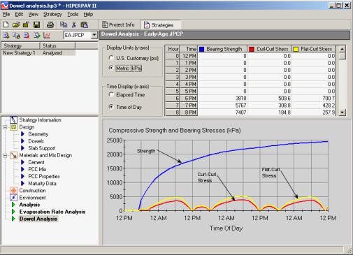
Figure 113. Dowel analysis screen for early-age JPCP.
The main focus of the software is in the early-age behavior of JPCP. The long-term performance module should be used to further optimize early-age pavement design, materials selection, and construction procedures. The long-term performance modeling should examine relative (strategy comparison) rather than absolute performance, based on early-age factors. In this way, the long-term module can reinforce good paving practices. It must not be used for pavement (structural) design purposes.
In this section, the long-term comparative analysis of early-age strategies is demonstrated. The user should be familiar with the early-age JPCP analysis screens before proceeding with this section.
After the user selects option 2 in the project type selection screen (figure 82), the software creates two early-age JPCP strategies with default inputs that the user can modify with the inputs for his or her specific situation.
In the example in figure 114, a limestone coarse aggregate is selected for the second strategy to observe the impact of this change in the long term as compared to the siliceous coarse aggregate used in the first strategy. The strategies are automatically sorted alphabetically. After both strategies have been analyzed, the user can switch to the long-term analysis module by selecting "LT JPCP" under the strategy type pulldown menu.
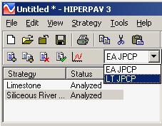
Figure 114. Strategy type pulldown menu.
After generating at least two early-age JPCP strategies and performing analyses on them, it is possible to run a long-term JPCP analysis.
This long-term analysis is designed to be comparative, so an early-age base strategy is selected and compared to the early-age comparison strategy. This allows the user to see how early-age factors affect long-term pavement performance. In this way, long-term performance effects can be reduced with the optimum selection of early-age factors.
Under strategy information, the user selects the base strategy and the comparison strategy (figure 115). Fields for user name and comments also are provided. After the strategy is run, the date of analysis will appear on this screen.
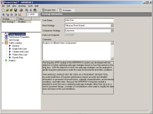
Figure 115. Strategy information for long-term JPCP analysis.
In the performance parameters screen, the user is able to enter the long-term analysis period, the reliability level, and the initial roughness index (figure 116). An option is also provided to assess the effect of built-in curling. Built-in curling is a term used for the curling state that develops at set and that later influences the curled shape of the slab as the thermal gradient is subsequently modified by the hydration process and climatic conditions (see section 2.4.2.2). HIPERPAV II considers two slab curling conditions:
In addition to the above inputs, the user can set the maximum allowable joint faulting, transverse cracking, longitudinal cracking, IRI, and serviceability in this input screen. These set limits are compared to the analysis results in the long-term analysis screen. If the analysis has predicted a level of distress that the user denotes as "terminating" (beyond the predefined distress threshold), HIPERPAV II reports it as the end of the service life for that analysis. However, the analysis continues until the analysis period is reached.
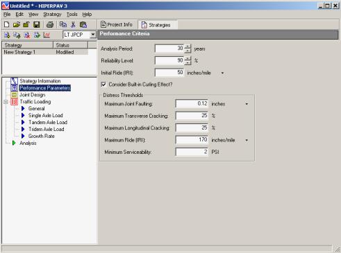
Figure 116. Performance criteria screen for long-term JPCP analysis.
Under the joint design the user selects weather dowels and tie bars are provided. Dowels reinforce the transverse joint while tie bars reinforce the longitudinal joint (figure 117).
Note: The inputs in the early-age dowel analysis module do not apply to the long-term analysis. If dowels are selected as the load-transfer device in the long-term analysis, then for every strategy, dowels are used in the analysis, regardless if they were used or not used in the early-age analysis.
The user can select from no transfer devices, only dowels, only tie-bars, or both dowels and tie bars. If dowels are selected, dowel spacing and length are required in addition to dowel size and modulus. If tie bars are selected, their size and spacing must be input. The transverse sawcut depth is also entered as part of the joint design inputs.
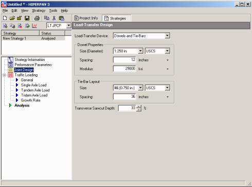
Figure 117. Load-transfer design for long-term JPCP analysis.
Traffic loading also must be input to the long-term analysis, in addition to the strategy information, distress thresholds, and load-transfer design input. Five input screens are provided for this category: one for general traffic information, three for traffic load spectra, and one for traffic growth rate.
In the general traffic input screen (figure 118), the mean truck tire pressure is required. The user can enter a user-defined traffic load spectra or have HIPERPAV II estimate the load spectra based on the input annual ESALs for the design lane. The default traffic load spectra generated by HIPERPAV II is based on typical averages of rural and urban highway traffic (see section B.2.5.4 in appendix B, volume III of this report series). If the user-defined option is selected, the user can enter specific single axle, tandem axle, or tridem axle load values in the gridlines for traffic loading.
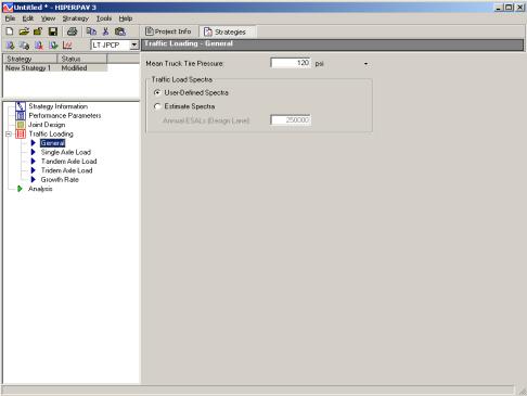
Figure 118. General traffic loading screen for long-term JPCP analysis.
If the user enters the load spectra information, this information is entered in the single axle load, the tandem axle load, and the tridem axle load screens (figure 119).
For each traffic load spectra category, the number of single tire and dual tire axle loads per year are entered against the axle load group. The single tire, dual tire, or total load spectra per axle type is shown on the plot, depending on the column selected. The total number of axles per axle load group is the sum of the respective single tire and dual tire values.
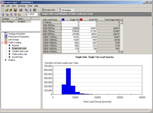
Figure 119. Single axle load screen for long-term JPCP analysis.
Finally, the traffic growth rate information is entered in the growth rate screen (figure 120). Three different growth functions can be specified: linear, exponential, or logistic. Depending on the function selected, the input required varies. For any function shown, the traffic loading is divided by the base-year traffic loading and plotted against time. Two plot methods may be selected: annual or cumulative.
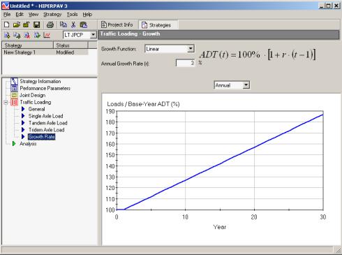
Figure 120. Traffic loading growth rate screen for long-term JPCP analysis.
With the input assigned, the user should save the project file before performing a long-term JPCP analysis. Icons to manipulate strategies similar to those available for early-age strategies can be used for long-term analyses (see section 7.2.1.1).
After the analysis is run, a window appears showing the analysis status. The base strategy first is analyzed followed by the comparison strategy (figure 121). For each strategy, several structural and functional distresses are predicted, including:
Each distress type is plotted as a function of time. The distress magnitudes are presented in tabular format at the end of the prediction lifetime or at the time the threshold value is reached, whichever occurs first.
Using the data values plot method, absolute values of the distress are provided (see plot method drop-down in figure 123. If the change plot method is chosen, the change in predicted distresses between the base strategy and the comparison strategy is plotted.
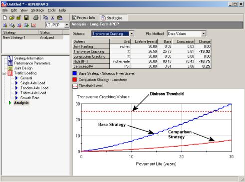
Figure 121. Analysis screen for long-term JPCP.
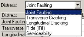
Figure 122. Drop-down menu for distress to plot.
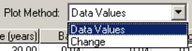
Figure 123. Plot method drop-down menu.
In the long-term module, if more than two early-age strategies are to be compared, this can be done by creating additional strategies with the strategy toolbar. Once the strategy is created, the additional strategies to compare are selected in the strategy information window, as previously described.
In this section, step-by-step instructions are provided to show the effect of aggregate selection on early-age thermal cracking potential and on long-term transverse cracking. The early-age inputs used for this exercise are presented in table 1. Input values in bold represent the inputs that are different for these two early-age strategies.
Table 1. Inputs for 11 a.m. and 7 p.m. times of placement strategies.
|
Input Category |
Input Screen |
Input Value |
|---|---|---|
|
Project Information |
Geography |
Austin, TX |
| Monthly Weather Data |
Estimate Monthly Data from Location |
|
| Strategy Information | Reliability Level |
90% |
Design |
Geometry |
New Slab Thickness = 250 mm New Slab Width = 3.65 m Transverse Joint Spacing = 4.5 m |
| Dowels Analysis |
Disabled |
|
| Slab Support |
Material Type = HMA (rough) k-value = 55 MPa/m Subbase Thickness = 15 mm Subbase Modulus = 3500 MPa Axial Restraint = Estimate from Material Type |
|
|
Materials and Mix Design |
Cement |
ASTM Cement Type Classification = Cement Type I Blaine Fineness Index = Estimate from Cement Type |
|
PCC Mix |
Aggregate Type = Siliceous River Gravel (Baseline Strategy) Limestone (Comparison Strategy) Admixtures = None Fly Ash Class = Class F (CaO <= 7.0% Coarse Aggregate = 1100 kg/m3 Fine Aggregate = 800 kg/m3 Water = 128 kg/m3 Cement = 284 kg/m3 Fly Ash = 60 kg/m3 GGBFS = 0 kg/m3 Silica Fume = 0 kg/m3 |
|
|
PCC Properties |
28-Day Splitting Tensile Strength = 3.2 MPa PCC 28-Day Modulus = 35,000 MPa PCC Ultimate Drying Shrinkage = Estimate from Mix PCC CTE = Estimate from Aggregate Type |
|
|
Maturity Data |
Default Strength Gain |
|
|
Construction |
Construction |
Initial PCC Mix Temperature = 32.2 °C Initial Support Layer Temperature = 31.7 °C Curing Method = Single Coat Curing Liquid Compound Age Curing Applied = 0 Hours Sawcutting: Saw at Optimum Time Skip Sawcutting: Not Used Strength for Opening to Traffic = Not Relevant for This Analysis |
|
Environment |
Environment |
Construction Date: July 18, 2002 (year irrelevant for analysis since temperatures are historical averages) Construction Time: 11:00 a.m. Temperature, Windspeed, Relative Humidity, and Cloud Cover = Estimate from Location |
To perform this analysis, a new long-term JPCP analysis is selected in the project type selection screen (see figure 82). The first step is to select the project location under the geography screen of the project information tab (see section 7.1). If not yet chosen, use the following icons in the geography toolbar to select Austin, TX, in the U.S. map (see figure 84):
 pin
pin
![]() zoom
zoom
![]() drag
drag
Next, select "Estimate monthly data from location" under the monthly weather data screen (see figure 85).
To enter the early-age inputs for the siliceous river gravel strategy, select the strategies tab (see figure 86). To rename this strategy "Siliceous River Gravel," right click on it and select "Rename," or select "Rename" from the strategy option on the HIPERPAV II top menu. Under "Strategy Information," the reliability level is set to 90 percent. In the same way, all other inputs shown in table 1 are entered under the design, materials and mix design, construction, and environment input screens. For this exercise, data for temperature, windspeed, relative humidity, and cloud cover are set to the default values estimated for that location.
After all the above inputs are entered, the user may perform
the analysis by clicking on the
 analysis icon of the strategy toolbar (see
section 7.2.1.1) or by selecting "Run Analysis" from the strategy
option on the HIPERPAV II top menu. The
results from this analysis are presented in figure 124. The results show a high risk of thermal
cracking for the siliceous river gravel strategy.
analysis icon of the strategy toolbar (see
section 7.2.1.1) or by selecting "Run Analysis" from the strategy
option on the HIPERPAV II top menu. The
results from this analysis are presented in figure 124. The results show a high risk of thermal
cracking for the siliceous river gravel strategy.
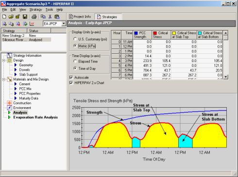
Figure 124. Analysis results for the siliceous river gravel strategy.
To proceed with the second strategy (using limestone coarse
aggregate), the user may either enter the information on a new strategy or
create a copy of the siliceous river gravel strategy. The later is recommended, since all previously entered data that
is identical for the second strategy will be automatically copied to the second
strategy. To do this, select the
siliceous river gravel strategy and click on the
 copy strategy icon. "Copy of Siliceous River Gravel Strategy" appears under the
strategy list. To rename this strategy
"Limestone," right click on it and select "Rename," or select "Rename" from the strategy option on the HIPERPAV II top menu.
copy strategy icon. "Copy of Siliceous River Gravel Strategy" appears under the
strategy list. To rename this strategy
"Limestone," right click on it and select "Rename," or select "Rename" from the strategy option on the HIPERPAV II top menu.
For the limestone strategy, change the aggregate type to limestone in the aggregate type drop-down menu under the PCC mix input screen (see figure 96).
After completing the inputs for the limestone strategy, perform the analysis by clicking on the analysis icon of the strategy toolbar. The result from this analysis is presented in figure 125. Less potential for thermal cracking is observed from the results of the limestone strategy as compared to the siliceous river gravel strategy.
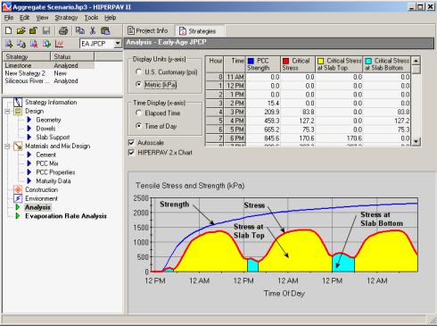
Figure 125. Analysis screen for limestone strategy.
After the two early-age strategies have been analyzed, the long-term analysis is performed using the inputs shown in table 2.
To begin the long-term analysis, select "LT JPCP" under the analysis type drop-down (see figure 114). Then, under "Strategy Information," select the siliceous river gravel early-age strategy as the base strategy and the limestone early-age strategy as the comparison strategy (see figure 126). Complete the rest of the input screens with the information provided in table 2.
Table 2. Long-term inputs for aggregate selection sample scenario.
| Input Category |
Input Screen |
Input
Value
|
|---|---|---|
| Strategy Information |
Strategy Information |
Base Strategy: Siliceous River Gravel Comparison Strategy: Limestone |
| Performance Parameters |
Performance Parameters |
Analysis Period: 30 Years Reliability Level: 90% Initial Ride: 0.8 m/km Consider Built-in Curling Effect: Yes Distress Thresholds: Maximum Joint Faulting: 3 mm Maximum Transverse Cracking: 25% Maximum Longitudinal Cracking: 25% Maximum Ride (IRI): 2.7 m/km Minimum Serviceability: 2.0 |
| Joint Design |
Joint Design |
Load Transfer Devices: Dowels and Tie-bars Dowel Properties: Size (Diameter): 32 mm Spacing: 300 mm Modulus: 200,000 MPa Tiebar Layout: Size: 19.1 mm Spacing: 0.9 m Transverse Sawcut Depth: 33% of Thickness |
| Traffic Loading |
General |
Mean Truck Tire Pressure: 0.84 MPa Traffic Load Spectra: Estimate Spectra from ESAL Annual ESAL (Design Lane): 250,000 |
| Single Axle Load |
Estimate from ESAL |
|
| Tandem Axle Load |
Estimate from ESAL |
|
| Tridem Axle Load |
Estimate from ESAL |
|
| Growth Rate |
Growth Function: Linear Annual Growth Rate: 3% Plot Method: Annual |
After all the inputs have been entered, the user may perform
the analysis by clicking on the  analysis icon of the strategy toolbar (see
section 7.2.1.1) or by selecting "Run Analysis" from the strategy
option on the HIPERPAV II top menu. The
joint faulting analysis is presented after the analysis is run. Transverse cracking may be selected from the
distress to plot drop-down menu (see figure 122). The transverse cracking results for the siliceous river gravel
and limestone early-age strategies are shown in figure 127. The strategy with siliceous river gravel
coarse aggregate shows a greater development of transverse cracking compared to
the strategy with limestone coarse aggregate. From this analysis, selecting the limestone coarse aggregate source with
a lower CTE appears to result in better performance, both in the early age and
in the long term.
analysis icon of the strategy toolbar (see
section 7.2.1.1) or by selecting "Run Analysis" from the strategy
option on the HIPERPAV II top menu. The
joint faulting analysis is presented after the analysis is run. Transverse cracking may be selected from the
distress to plot drop-down menu (see figure 122). The transverse cracking results for the siliceous river gravel
and limestone early-age strategies are shown in figure 127. The strategy with siliceous river gravel
coarse aggregate shows a greater development of transverse cracking compared to
the strategy with limestone coarse aggregate. From this analysis, selecting the limestone coarse aggregate source with
a lower CTE appears to result in better performance, both in the early age and
in the long term.
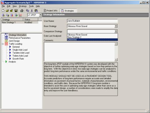
Figure 126. Selection of early-age strategies to compare.
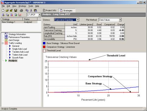
Figure 127. Long-term strategy transverse cracking results.
In this section, the analysis for an early-age CRCP project is demonstrated.
After the user selects option 3 in the project type selection screen (figure 82), the software creates an early-age CRCP strategy with default inputs that the user can modify with the inputs for the specific situation. The input screens are similar to those required for the early-age JPCP analysis, with some differences.
After the general project information is entered, as shown in section 7.1, one or more strategies for that specific location can be created for analysis under the strategies section.
The strategies section contains, in tree view, the specific input data required to perform an early-age CRCP analysis under the categories of:
For information on the strategy toolbar, see section 7.2.1.1.
Under the strategy information screen, the user can enter his or her name. After the strategy is run, the date of analysis also will appear on this screen. A comment box is available for each strategy. This screen is similar to the strategy information screen for early-age JPCP analyses, although no reliability information is required (see figure 86).
Under the design inputs, the user can enter the pavement design information, including pavement geometry, steel design, and slab support information.
The geometry screen (figure 128) provides fields to enter the slab thickness and slab width. The slab width that should be input in HIPERPAV II is the widest spacing between adjacent longitudinal joints.
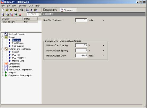
Figure 128. Geometry screen for early-age CRCP analysis.
In addition, long-term desirable CRCP cracking characteristics (after 1 year), including minimum and maximum crack spacing and average crack width, can be entered; these later will be shown by the dashed lines in the early-age CRCP analysis plot.
The longitudinal steel information can be input to the program in the steel design screen (figure 129). Information about the longitudinal steel layout and steel properties is required. For the steel layout, the bar spacing and size are needed, as well as the number of steel mats. The steel properties needed are the steel yield strength, steel modulus, and CTE. HIPERPAV II then calculates, based on the input, the percent steel for the current slab thickness.
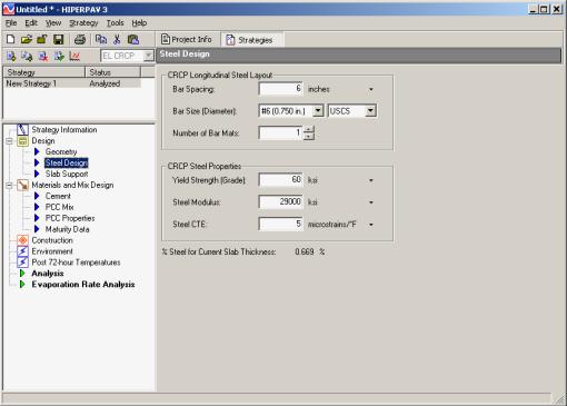
Figure 129. Steel design screen for early-age CRCP analysis.
For information about this screen, see section 7.2.2.3.
The second input category is materials and mix design (see section 7.2.3)
The third input category corresponds to construction information. The construction screen for the early-age CRCP analysis is shown in figure 130. In this screen, the initial temperatures of the concrete mix and support layer are entered. Information on the curing method used (pulldown) is required along with the time of application, and if removable curing methods are selected, the age when curing is removed also is required.
In addition, if the effect of construction traffic is enabled, loading conditions are required. The user can assess the influence of construction traffic on the performance of the CRCP by inputting the days before the wheel load is applied, the wheel load, and the radius of the circular loaded area.
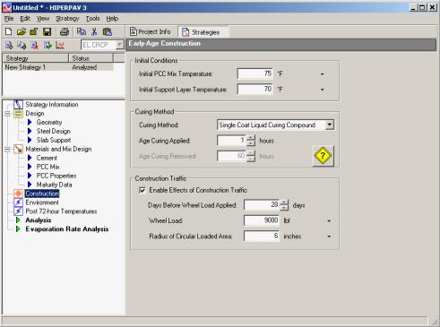
Figure 130. Early-age construction screen for early-age CRCP analysis.
The environment screen is the same as the early-age JPCP screen seen in section .
For the early-age CRCP analysis, the post 72-hour temperatures are required (figure 131). The user may estimate these inputs using the HIPERPAV II environmental database, or the user can define them. The critical analysis period corresponds to the time when construction traffic is applied. For this period, the minimum and maximum air temperatures are also required. In addition, after the critical analysis period, the date of the minimum temperature for the year is needed to estimate the pavement age for the largest temperature drop to which the pavement will be subjected. This date can be estimated by HIPERPAV II, or it can be defined by the user. Similarly, HIPERPAV II can either estimate the minimum and maximum temperatures, or these can be input.
Early age in HIPERPAV II includes the first 72 hours after construction for both JPCP and CRCP. Cracking in CRCP typically progresses until approximately 1 year after construction. After 1 year, cracking typically remains constant. The HIPERPAV II analysis extends beyond early age up to 1 year (early life) to realistically assess the behavior of CRC pavements inservice.
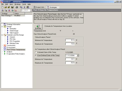
Figure 131. Post 72-hour air temperatures screen for early-age CRCP analysis.
With the input assigned, the user should save the file before performing an early-age CRCP analysis. The analysis screen for an early-age CRCP strategy is shown in figure 132. After the analysis is run, a window appears showing the analysis status. The analysis output, in tabular format, includes the average crack spacing and its standard deviation, the average crack width, the maximum steel stress, and the bond development length. Interpretation of the analysis is performed by comparing the cracking results with the thresholds previously set in "Desirable CRCP Cracking Characteristics" in the geometry input screen. These thresholds are also presented in the analysis screen for comparison.
The plot can either show the incremental or cumulative frequency versus crack spacing. Plots for three different points in time are provided: 1) at 3 days after construction; 2) for the critical analysis period when construction traffic is applied; and 3) at 1 year of age ("Time Period to Plot" pulldown in figure 133). The crack spacing frequency also is presented in tabular format. The numerical value of crack spacing frequency can also be obtained by hovering the mouse over the point of interest in the plot. As shown in figure 134, a help window is provided to caution the user on the validation of the crack width model incorporated in HIPERPAV II. This window also defines the analysis period used for CRCP behavior analyses.
Also, because more than one strategy can be analyzed with HIPERPAV II, comparisons can be made between the analysis results more easily. It is possible to toggle between the analysis screens by selecting one strategy and then the other one (for this, the user must have analyzed at least two strategies previously for comparison and toggled between them).
An analysis screen also is provided for evaporation rate. The evaporation rate analysis is the same as for the early-age JPCP (see section 7.2.6.2).
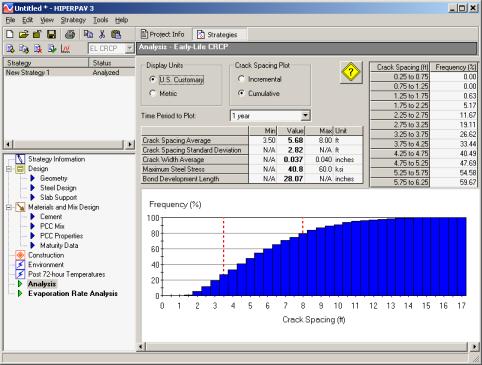
Figure 132. Analysis screen for early-age CRCP.
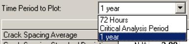
Figure 133. Drop-down menu for time period to plot.
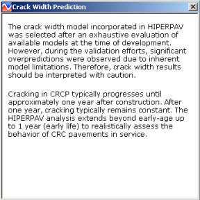
Figure 134. Help icon under CRCP analysis screen.
One of the objectives of the CRCP analysis is to achieve a crack spacing distribution that falls within the predefined thresholds, with only a small percentage of cracks falling above and/or below the maximum and minimum crack spacing limits, respectively, as shown in figure 132. In this analysis, both crack width and crack spacing are within acceptable limits. An example of a CRCP analysis with poor cracking characteristics is shown in figure 135. In this second analysis, neither crack spacing nor crack width fall within acceptable limits. In addition, a large percentage of crack spacings fall below the predefined minimum crack spacing threshold.
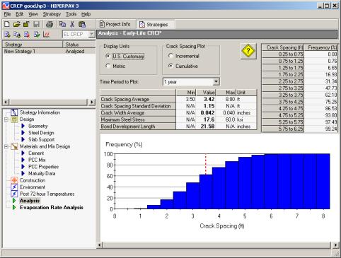
Figure 135. CRCP analysis with poor cracking characteristics.
It is also recommended to compare the maximum steel stress predicted with the steel yield strength to evaluate the potential of wide cracks or steel rupture. The bond development length is predicted to compare with the predicted crack spacing. The user should achieve a minimum average crack spacing of twice the bond development length to ensure good CRCP behavior. For additional information on CRCP behavior, refer to section.
For any HIPERPAV II analysis, reports can be generated by clicking on the print icon on the upper icon toolbar or by selecting "Print" from the file menu. After selecting "Print," a HIPERPAV II report screen is displayed as shown in figure 136. In this screen, options are available to select printing options under the setup icon, send the report to the printer as-is under the print icon, preview the report under the preview icon, and export the results to a Microsoft Excel spreadsheet under the export icon.
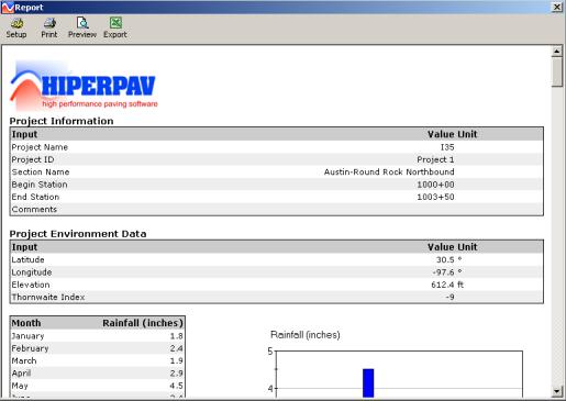
Figure 136. HIPERPAV II report screen.
The Concrete Optimization, Management, Engineering, and Testing (COMET) module is a simplified derivation of the Concrete Optimization Software Tool (COST) that was developed by FHWA and the National Institute of Standards and Technology (NIST) for optimizing concrete mixes. COMET can be accessed within HIPERPAV II by selecting "COMET" in the tools top menu bar shown in figure 137. COMET optimizes concrete mixes based on early-age strength, 28-day strength, and cost.
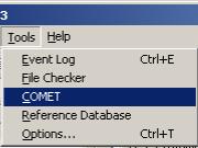
Figure 137. Tools drop-down menu in HIPERPAV II.
Once selected, the COMET initial window appears as shown in figure 138. Inputs and outputs can be selected on the tree view on the left side of the screen. The inputs for the screen selected are displayed on the right. The first item on the tree view, "Event Log," reports potential problems that may arise while running the software. Also, the tree view shows two levels of inputs and outputs. Level 1 inputs generate the experiment design of trial batches required for optimization. Level 2 inputs produce a set of optimum mixes based on the trial batch test results, and desirability functions defined for each response (early-age strength, 28-day strength, and cost).
As shown in figure 138, mix constituents are limited to cement, pozzolan, water, coarse aggregate, and fine aggregate. For each constituent, the specific gravity and cost is required.
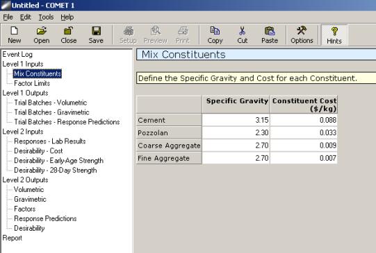
Figure 138. Mix constituents input screen in COMET.
The user provides optimization ranges for coarse aggregate fraction, cementitious content, pozzolan substitution, and w/cm ratio (see figure 139).
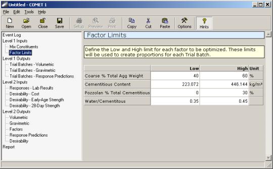
Figure 139. Factor limits input screen in COMET.
With the inputs in level 1, trial batches are developed for the experimental program by running the "Create Trial Batches" command button in the level 1 outputs screen, as shown in figure 140. As a result, 29 trial batches are generated, which can be displayed in volumetric (percent of total volume) and gravimetric (weight per unit of volume) form. The gravimetric form is presented in figure 141.
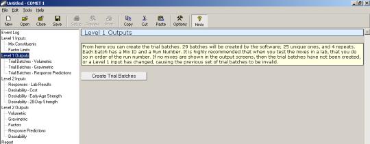
Figure 140. Create trial batches command button in level 1 outputs.
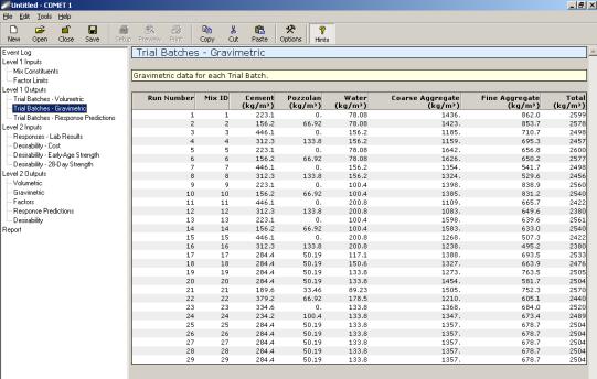
Figure 141. Trial batches in kg/m3, gravimetric form.
In addition, as shown in figure 142, the cost for every trial batch is computed and default models in COMET are used to predict early-age strength and 28-day strength as a function of mix constituents. Predicted responses are only approximate and may be used in a planning stage in which the mix constituents may not be known or are not available for testing.
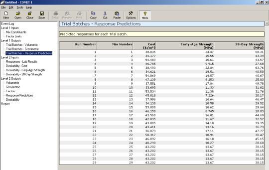
Figure 142. Predicted responses for each trial batch.
After the level 1 inputs and outputs are complete, the user can proceed with level 2 analysis. To continue with this analysis, the user must enter the laboratory testing results for each response for the trial batches generated in level 1 (see figure 143). Alternatively, the user may fill in these values using default models by clicking on the "Reset to Predicted Values" command button, if a preliminary analysis is desirable.
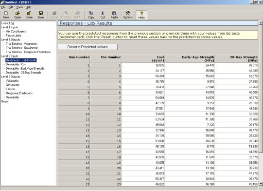
Figure 143. Lab results screen.
The user can assign desirability functions for each of the optimization responses under the cost, early-age strength, and 28-day strength desirability screens (a sample desirability function is shown in figure 144 for 28-day strength).
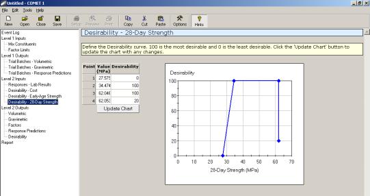
Figure 144. Desirability function for 28-day strength.
After the level 2 inputs are entered, optimization of mixes is performed by clicking the "Optimize Mixes" command button in the level 2 outputs screen (see figure 145). With this command, regression models based on the results from the experimental program or from the predicted responses are developed as a function of the mix proportions.
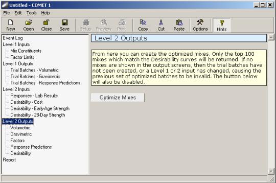
Figure 145. Level 2 outputs—command to optimize mixes.
These models predict responses for a comprehensive set of mixtures within the factor limits specified in the factor limits screen. Finally, optimum mixes are identified in terms of the individual desirability for every response and the maximum overall desirability for all responses, and are presented in volumetric and gravimetric form. Optimum mixes are shown in volumetric form in figure 146.
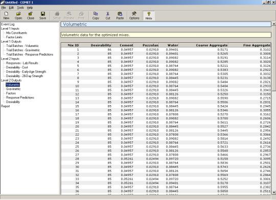
Figure 146. Optimum mixes sorted by desirability in volumetric form.
In addition, the optimum mixes are also displayed in terms of the optimization factors, predicted responses, and individual response desirabilities as shown in figures 147, 148, and 149, respectively.
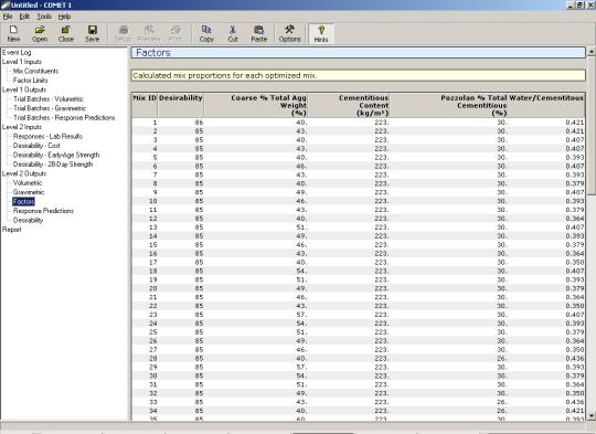
Figure 147. Optimum mixtures in terms of optimization factors.
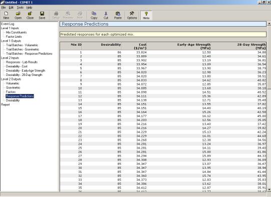
Figure 148. Response predictions for optimum mixtures.
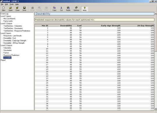
Figure 149. Individual response desirabilities for optimum mixtures.
A report that can be used for printing the inputs and outputs for the entire analysis is generated, as shown in figure 150. To print, click on the print icon on the upper icon toolbar.
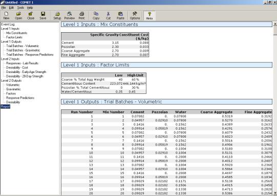
Figure 150. Report view for printing purposes.


 Zoom to show the entire map.