U.S. Department of Transportation
Federal Highway Administration
1200 New Jersey Avenue, SE
Washington, DC 20590
202-366-4000
Federal Highway Administration Research and Technology
Coordinating, Developing, and Delivering Highway Transportation Innovations
 |
| This report is an archived publication and may contain dated technical, contact, and link information |
|
Publication Number: FHWA-HRT-04-127 Date: January 2006 |
Previous | Table of Contents | Next
Four field sites were investigated for validation of the HIPERPAV II system:
It is believed that the number of field sites evaluated will provide the minimum level of information necessary to meet the objectives of this effort successfully. However, future data from field sites could be used for local customization. This section describes the steps performed for validation of both the JPCP and CRCP pavement sites investigated.
JPCP sites investigated include a section on U.S. Highway 50 in Illinois and a bypass section of a farm to market road near Ticuman, Mexico. The selection of both sites was heavily weighted on the fact that extensive early-age and performance information is available for both of these sections.
A field investigation and monitoring of a JPCP test section on U.S. Highway 50 near Carlyle, IL, was performed from August 7-10, 2001. Following is some background information on this section.
The test sections were constructed and instrumented from April to August in 1986 on U.S. Highway 50 just west of Carlyle, IL. Early-age monitoring was performed by researchers at the University of Illinois at Urbana-Champaign.(103) These data were used to develop mechanistic design procedures for the Illinois DOT. The following tables and figures provide a brief summary of the published data. Table 41 gives a brief description of the JPCP test sections.
| Section | Design Thickness (mm) | Underdrains | Sealed Edge Joint | Section Length (m) |
|---|---|---|---|---|
| AA | 241 | Y | N | 304 |
| IA | 216 | N | Y | 311 |
| JA | 216 | N | Y | 305 |
| KA | 216 | Y | Y | 305 |
| LA | 216 | Y | N | 335 |
| MA | 191 | Y | Y | 335 |
| NA | 191 | Y | N | 305 |
Section AA borders a bridge abutment on the west and is located 4.8 km from the other sections, which run continuously between IA to NA from west to east. The JPCP sections in this study were constructed with 6.1-m dowelled transverse joints. A 102-mm cement aggregate mixture (CAM) was used as the subbase. The concrete mix design was kept constant throughout the test sections and is shown in table 42.
| Constituent | Description | Quantity |
|---|---|---|
| Cement | Continental cement | 341 kg/m2 |
| Coarse aggregate | Falling springs quarry 022CAM07 | 1121 kg/m2 |
| Fine aggregate | Keyesport sand and gravel #2 027FAM01 | 666 kg/m2 |
| Water | - | 148 kg/m2 |
| Air entrainment | Darex | - |
| Water reducer | Type A—WRDA® with Hycol | - |
| w/c | - | 0.43 |
| Mortar factor | - | 0.80 |
Strength gain data were reported by Zollinger and Barenberg.(103) The reported centerpoint loading flexural strength at 28 days showed an average of 5.8 MPa, and the third point loading flexural strength at 28 days showed an average of 4.9 MPa. The average 28-day modulus of elasticity for all sections is 28,680 MPa.
Table 43 contains traffic data for each test section between 1987 and 1999 provided by Illinois DOT. This table shows the accumulation of ESALs for all sections. In this analysis, the traffic is divided into vehicular categories and factors to calculate ESALs.
| Year | Average Daily Traffic | Heavy Commercial Vehicles | Multiple Unit Vehicles | Single Unit Vehicles | Passenger Vehicles | MU Factor | SU Factor | PV Factor | Distribution Factor | ESALs (106) |
|---|---|---|---|---|---|---|---|---|---|---|
| 1987 | 3400 | 461 | 340 | 121 | 2939 | 567.21 | 135.78 | 0.15 | 0.5 | 0.10 |
| 1988 | 4175 | 475 | 350 | 125 | 3700 | 567.21 | 135.78 | 0.15 | 0.5 | 0.11 |
| 1989 | 4950 | 594 | 338 | 256 | 4356 | 567.21 | 135.78 | 0.15 | 0.5 | 0.11 |
| 1990 | 4875 | 713 | 325 | 388 | 4162 | 567.21 | 135.78 | 0.15 | 0.5 | 0.12 |
| 1991 | 4800 | 831 | 313 | 519 | 3969 | 567.21 | 135.78 | 0.15 | 0.5 | 0.12 |
| 1992 | 4750 | 950 | 300 | 650 | 3800 | 567.21 | 135.78 | 0.15 | 0.5 | 0.13 |
| 1993 | 4700 | 900 | 350 | 550 | 3800 | 567.21 | 135.78 | 0.15 | 0.5 | 0.14 |
| 1994 | 4800 | 850 | 400 | 450 | 3950 | 567.21 | 135.78 | 0.15 | 0.5 | 0.14 |
| 1995 | 4900 | 800 | 450 | 350 | 4100 | 567.21 | 135.78 | 0.15 | 0.5 | 0.15 |
| 1996 | 5000 | 750 | 500 | 250 | 4250 | 567.21 | 135.78 | 0.15 | 0.5 | 0.16 |
| 1997 | 5100 | 773 | 515 | 258 | 4327 | 567.21 | 135.78 | 0.15 | 0.5 | 0.16 |
| 1998 | 5253 | 796 | 530 | 265 | 4457 | 567.21 | 135.78 | 0.15 | 0.5 | 0.17 |
| 1999 | 5411 | 820 | 546 | 273 | 4591 | 567.21 | 135.78 | 0.15 | 0.5 | 0.17 |
| Total | 1.80 | |||||||||
Table 44 compares the design ESALs versus the consumed ESALs as of 1999. All sections but section AA had surpassed the number of design ESALs by 1999. Sections MA and NA had nearly three times the number of design ESALs by 1999.
| Section | Design ESALS | 1999 Cumulative ESALs | Percent Consumed |
|---|---|---|---|
| AA | 2.60 | 1.80 | 69.1 |
| IA | 1.50 | 1.80 | 119.8 |
| JA | 1.50 | 1.80 | 119.8 |
| KA | 1.50 | 1.80 | 119.8 |
| LA | 1.50 | 1.80 | 119.8 |
| MA | 0.64 | 1.80 | 280.8 |
| NA | 0.64 | 1.80 | 280.8 |
Table 45 gives friction and ride quality data for the test sections at different times between 1990 and 1999, from Illinois DOT records.
| Year | Age (years) | IRI (m/km) |
|---|---|---|
| 1994 | 8 | 1.53 |
| 1996 | 10 | 1.82 |
| 1998 | 12 | 1.78 |
Illinois DOT performed falling weight deflectometer (FWD) tests on the test sections in 1994 and 1998. Table 46 gives the results for D0, deflection under the load, and LTE.
| Section | Year | D0 (microns) |
Design Thickness |
LTE, Transverse (%) | LTE, Shoulder (%) | LTE, Cracks (%) |
|---|---|---|---|---|---|---|
| AA | 1994 | 86.4 | 241 mm | 92.9 | 93.3 | N/A |
| 1998 | 66.0 | 83.8 | 76.4 | N/A | ||
| IA | 1994 | 121.9 | 216 mm | 85.1 | 70.8 | N/A |
| 1998 | 106.7 | 83.9 | 61.7 | N/A | ||
| JA | 1994 | 127.0 | 216 mm | 83.4 | 81.3 | 87.9 |
| 1998 | 109.2 | 84.9 | 51.0 | 61.6 | ||
| LA | 1994 | 104.1 | 216 mm | 91.7 | 89.8 | N/A |
| 1998 | 104.1 | 85.4 | 68.1 | N/A | ||
| NA | 1994 | 139.7 | 191 mm | 89.8 | 75.3 | 88.0 |
| 1998 | 139.7 | 82.8 | 64.0 | 81.0 |
N/A = Not applicable (no cracks observed)
Before construction, the modulus of subgrade reaction was determined at several locations along the site and reported by Zollinger and Barenberg. An average static k-value of 130 psi was observed, although no test date was reported.(103)
In addition, historical condition survey data for the seven test sections were obtained from Illinois DOT and are presented in tables 47 through 53. In summary, each section remains intact, with the only visible distresses being a very small amount of transverse cracking and construction joint deterioration in several sections and some patching in section IA. The sections are performing well, considering the level of ESALs and the age of the pavements.
| Distress | Units | Severity | Year | ||||
|---|---|---|---|---|---|---|---|
| 1990 | 1992 | 1995 | 1997 | 2001 | |||
| Corner break | Number | Low | 0 | 0 | 0 | 0 | 0 |
| Medium | 0 | 0 | 0 | 0 | 0 | ||
| High | 0 | 0 | 0 | 0 | 0 | ||
| Longitudinal cracking | Lane feet | Low | 0 | 0 | 0 | 0 | 0 |
| Medium | 0 | 0 | 0 | 0 | 0 | ||
| High | 0 | 0 | 0 | 0 | 0 | ||
| Random longitudinal cracking | Lane feet | Low | 0 | 0 | 0 | 0 | 1 |
| Medium | 0 | 0 | 0 | 0 | 0 | ||
| High | 0 | 0 | 0 | 0 | 0 | ||
| Spalling | Number | Low | 0 | 0 | 0 | 0 | 17 |
| Medium | 0 | 0 | 0 | 0 | 0 | ||
| High | 0 | 0 | 0 | 0 | 0 | ||
| Transverse cracking | Number | Low | 0 | 0 | 0 | 0 | 0 |
| Medium | 0 | 0 | 0 | 0 | 0 | ||
| High | 0 | 0 | 0 | 0 | 0 | ||
* Data provided by Illinois DOT
| Distress | Units | Severity | Year | ||||
|---|---|---|---|---|---|---|---|
| 1990 | 1992 | 1995 | 1997 | 2001 | |||
| Corner break | Number | Low | 0 | 0 | 0 | 0 | 0 |
| Medium | 0 | 0 | 0 | 0 | 0 | ||
| High | 0 | 0 | 0 | 0 | 0 | ||
| Longitudinal cracking | Lane feet | Low | 0 | 0 | 0 | 0 | 0 |
| Medium | 0 | 0 | 0 | 0 | 0 | ||
| High | 0 | 0 | 0 | 0 | 0 | ||
| Patching | Lane feet | Low | 96 | 96 | 96 | 96 | 0 |
| Medium | 0 | 0 | 0 | 0 | 0 | ||
| High | 0 | 0 | 0 | 0 | 0 | ||
| Random longitudinal cracking | Lane feet | Low | 0 | 0 | 0 | 0 | 0 |
| Medium | 0 | 0 | 0 | 0 | 0 | ||
| High | 0 | 0 | 0 | 0 | 0 | ||
| Spalling | Number | Low | 1 | 1 | 1 | 1 | 2 |
| Medium | 0 | 0 | 0 | 0 | 0 | ||
| High | 0 | 0 | 0 | 0 | 0 | ||
| Transverse cracking | Number | Low | 2 | 2 | 0 | 0 | 0 |
| Medium | 2 | 2 | 4 | 4 | 0 | ||
| High | 0 | 0 | 0 | 0 | 2 | ||
* Data provided by Illinois DOT
| Distress | Units | Severity | Year | ||||
|---|---|---|---|---|---|---|---|
| 1990 | 1992 | 1995 | 1997 | 2001 | |||
| Corner break | Number | Low | 0 | 0 | 0 | 0 | 0 |
| Medium | 0 | 0 | 0 | 0 | 1 | ||
| High | 0 | 0 | 0 | 0 | 0 | ||
| Longitudinal cracking | Lane feet | Low | 0 | 0 | 0 | 0 | 0 |
| Medium | 0 | 0 | 0 | 0 | 0 | ||
| High | 0 | 0 | 0 | 0 | 0 | ||
| Patching | Lane feet | Low | 0 | 0 | 0 | 0 | 0 |
| Medium | 0 | 0 | 0 | 0 | 0 | ||
| High | 0 | 0 | 0 | 0 | 0 | ||
| Random longitudinal cracking | Lane feet | Low | 0 | 0 | 0 | 0 | 0 |
| Medium | 0 | 0 | 0 | 0 | 0 | ||
| High | 0 | 0 | 0 | 0 | 0 | ||
| Spalling | Number | Low | 0 | 0 | 2 | 0 | 1 |
| Medium | 1 | 1 | 0 | 1 | 0 | ||
| High | 0 | 0 | 0 | 0 | 0 | ||
| Transverse cracking | Number | Low | 0 | 0 | 3 | 2 | 0 |
| Medium | 4 | 6 | 3 | 6 | 1 | ||
| High | 0 | 0 | 0 | 0 | 5 | ||
* Data provided by Illinois DOT
| Distress | Units | Severity | Year | ||||
|---|---|---|---|---|---|---|---|
| 1990 | 1992 | 1995 | 1997 | 2001 | |||
| Corner break | Number | Low | 0 | 0 | 0 | 0 | 0 |
| Medium | 0 | 0 | 0 | 0 | 0 | ||
| High | 0 | 0 | 0 | 0 | 0 | ||
| Longitudinal cracking | Lane feet | Low | 0 | 0 | 0 | 0 | 0 |
| Medium | 0 | 0 | 0 | 0 | 0 | ||
| High | 0 | 0 | 0 | 0 | 0 | ||
| Patching | Lane feet | Low | 0 | 0 | 0 | 0 | 0 |
| Medium | 0 | 0 | 0 | 0 | 0 | ||
| High | 0 | 0 | 0 | 0 | 0 | ||
| Random longitudinal cracking | Lane feet | Low | 0 | 0 | 0 | 0 | 0 |
| Medium | 0 | 0 | 0 | 0 | 0 | ||
| High | 0 | 0 | 0 | 0 | 0 | ||
| Spalling | Number | Low | 0 | 0 | 0 | 0 | 5 |
| Medium | 0 | 0 | 0 | 0 | 2 | ||
| High | 0 | 0 | 0 | 0 | 0 | ||
| Transverse cracking | Number | Low | 1 | 1 | 0 | 0 | 0 |
| Medium | 0 | 0 | 0 | 0 | 0 | ||
| High | 0 | 0 | 0 | 0 | 0 | ||
* Data provided by Illinois DOT
| Distress | Units | Severity | Year | ||||
|---|---|---|---|---|---|---|---|
| 1990 | 1992 | 1995 | 1997 | 2001 | |||
| Corner break | Number | Low | 0 | 0 | 0 | 0 | 0 |
| Medium | 0 | 0 | 0 | 0 | 0 | ||
| High | 0 | 0 | 0 | 0 | 0 | ||
| Longitudinal cracking | Lane feet | Low | 0 | 0 | 0 | 0 | 0 |
| Medium | 0 | 0 | 0 | 0 | 0 | ||
| High | 0 | 0 | 0 | 0 | 0 | ||
| Patching | Lane feet | Low | 0 | 0 | 0 | 0 | 0 |
| Medium | 0 | 0 | 0 | 0 | 0 | ||
| High | 0 | 0 | 0 | 0 | 0 | ||
| Random longitudinal cracking | Lane feet | Low | 0 | 0 | 0 | 0 | 0 |
| Medium | 0 | 0 | 0 | 0 | 0 | ||
| High | 0 | 0 | 0 | 0 | 0 | ||
| Spalling | Number | Low | 0 | 0 | 0 | 0 | 5 |
| Medium | 0 | 0 | 0 | 0 | 6 | ||
| High | 0 | 0 | 0 | 0 | 0 | ||
| Transverse cracking | Number | Low | 7 | 7 | 0 | 0 | 0 |
| Medium | 0 | 0 | 0 | 0 | 0 | ||
| High | 0 | 0 | 0 | 0 | 0 | ||
* Data provided by Illinois DOT
| Distress | Units | Severity | Year | ||||
|---|---|---|---|---|---|---|---|
| 1990 | 1992 | 1995 | 1997 | 2001 | |||
| Corner break | Number | Low | 0 | 0 | 0 | 0 | 0 |
| Medium | 0 | 0 | 0 | 0 | 0 | ||
| High | 0 | 0 | 0 | 0 | 0 | ||
| Longitudinal cracking | Lane feet | Low | 0 | 0 | 0 | 0 | 0 |
| Medium | 0 | 0 | 0 | 0 | 0 | ||
| High | 0 | 0 | 0 | 0 | 0 | ||
| Patching | Lane feet | Low | 0 | 0 | 0 | 0 | 0 |
| Medium | 0 | 0 | 0 | 0 | 0 | ||
| High | 0 | 0 | 0 | 0 | 0 | ||
| Random longitudinal cracking | Lane feet | Low | 0 | 0 | 0 | 0 | 0 |
| Medium | 0 | 0 | 0 | 0 | 0 | ||
| High | 0 | 0 | 0 | 0 | 0 | ||
| Spalling | Number | Low | 0 | 0 | 0 | 0 | 5 |
| Medium | 0 | 0 | 0 | 0 | 0 | ||
| High | 0 | 0 | 0 | 0 | 0 | ||
| Transverse cracking | Number | Low | 0 | 2 | 0 | 0 | 0 |
| Medium | 0 | 0 | 0 | 0 | 0 | ||
| High | 0 | 0 | 0 | 0 | 0 | ||
* Data provided by Illinois DOT
| Distress | Units | Severity | Year | ||||
|---|---|---|---|---|---|---|---|
| 1990 | 1992 | 1995 | 1997 | 2001 | |||
| Corner break | Number | Low | 0 | 0 | 0 | 0 | 0 |
| Medium | 0 | 0 | 0 | 0 | 1 | ||
| High | 0 | 0 | 0 | 0 | 0 | ||
| Longitudinal cracking | Lane feet | Low | 0 | 0 | 0 | 0 | 1 |
| Medium | 0 | 0 | 0 | 0 | 0 | ||
| High | 0 | 0 | 0 | 0 | 0 | ||
| Patching | Lane feet | Low | 0 | 0 | 0 | 0 | 0 |
| Medium | 0 | 0 | 0 | 0 | 0 | ||
| High | 0 | 0 | 0 | 0 | 0 | ||
| Random longitudinal cracking | Lane feet | Low | 0 | 0 | 0 | 0 | 0 |
| Medium | 0 | 0 | 0 | 0 | 0 | ||
| High | 0 | 0 | 0 | 0 | 0 | ||
| Spalling | Number | Low | 0 | 0 | 0 | 0 | 17 |
| Medium | 0 | 0 | 0 | 0 | 0 | ||
| High | 0 | 0 | 0 | 0 | 0 | ||
| Transverse cracking | Number | Low | 3 | 6 | 5 | 5 | 0 |
| Medium | 0 | 1 | 4 | 4 | 1 | ||
| High | 3 | 3 | 2 | 3 | 7 | ||
* Data provided by Illinois DOT
The monitoring included the following activities:
The data collected from this experiment were used with early-age information available for this site to validate the long-term JPCP performance models in HIPERPAV II.
A condition survey with photo and video documentation for all seven test sections was performed during the afternoon of August 7, 2001. The location and severity of each distress was documented. As in the historical condition survey data, few distresses were evident in the sections. The major distresses included a few slabs with transverse cracking and some low severity transverse joint spalling. The pavement has performed well, considering all sections except section AA exceeded the number of design ESALs by 1999, according to the original design.
Sections AA, IA, JA, KA, and LA were tested with FWD at midslab for backcalculation of the modulus of subgrade reaction (k) and at transverse and longitudinal shoulder joints for LTE. Each test consisted of a seating drop followed by drops at three increasing loads, typically near 9, 12, and 15 kips. The approach and leave sides of transverse joints were tested. Table 54 provides a summary of center slab deflection bowls that have been normalized to 9 kips and are compared to historical deflections in 1994 and 1998.
| Section | Statistic | 0 mm (1994) | 0 mm (1998) | 0 mm | 304.8 mm | 609.6 mm | 914.4 mm | 1219.2 mm | 1524 mm | 1829 mm |
|---|---|---|---|---|---|---|---|---|---|---|
| AA | Mean | 86.4 | 66.0 | 67.8 | 62.2 | 54.1 | 46.7 | 39.4 | 33.3 | 28.2 |
| St. Dev | - | - | 5.6 | 4.8 | 3.6 | 2.8 | 2.0 | 1.5 | 1.0 | |
| IA | Mean | 121.9 | 106.7 | 135.6 | 123.4 | 106.4 | 88.6 | 72.4 | 57.4 | 43.7 |
| St. Dev | - | - | 26.7 | 23.1 | 17.3 | 12.7 | 9.1 | 6.6 | 4.3 | |
| JA | Mean | 127.0 | 109.2 | 131.6 | 124.0 | 110.5 | 93.0 | 78.0 | 62.2 | 47.2 |
| St. Dev | - | - | 4.3 | 4.3 | 5.1 | 5.1 | 5.1 | 4.6 | 3.8 | |
| KA | Mean | N/A | N/A | 121.2 | 112.8 | 99.3 | 84.6 | 71.9 | 59.2 | 47.5 |
| St. Dev | - | - | 16.3 | 14.2 | 9.9 | 5.1 | 2.0 | 2.5 | 2.3 | |
| LA | Mean | 104.1 | 104.1 | 128.0 | 121.9 | 106.7 | 92.7 | 75.9 | 61.5 | 48.8 |
| St. Dev | - | - | 16.0 | 13.7 | 9.7 | 6.6 | 3.0 | 2.0 | 1.0 |
Table 55 contains load transfer data and statistics for transverse joints for approach slabs.
| Section | Avg. Load (N) | Load Transfer Efficiency | |||||
|---|---|---|---|---|---|---|---|
| 1994 (%) | 1998 (%) | Mean (%) | St. Dev (%) | Median (%) | 15th Percentile (%) | ||
| AA | 39 | 92.9 | 83.8 | 77.3 | 1.41 | 77.2 | 76.1 |
| 52 | 77.1 | 1.01 | 76.8 | 76.2 | |||
| 66 | 77.1 | 1.08 | 77.0 | 76.3 | |||
| IA | 40 | 85.1 | 83.9 | 80.4 | 1.17 | 80.3 | 79.4 |
| 53 | 80.2 | 1.44 | 80.3 | 78.8 | |||
| 68 | 80.0 | 1.38 | 80.3 | 78.7 | |||
| JA | 39 | 83.4 | 84.9 | 81.2 | 1.32 | 81.6 | 80.0 |
| 52 | 80.9 | 0.60 | 80.7 | 80.4 | |||
| 67 | 80.6 | 0.74 | 80.7 | 79.9 | |||
| KA | 39 | N/A | N/A | 81.6 | 1.06 | 81.4 | 80.9 |
| 51 | 81.7 | 0.89 | 81.6 | 81.0 | |||
| 66 | 81.9 | 1.17 | 81.6 | 81.0 | |||
| LA | 38 | 91.7 | 85.4 | 82.5 | 0.56 | 82.6 | 82.0 |
| 50 | 83.2 | 0.99 | 83.5 | 82.3 | |||
| 65 | 82.7 | 0.78 | 83.2 | 81.8 | |||
| Cracks ( Section IA ) | 39 | N/A | N/A | 79.6 | 0.06 | Not enough data (two values) | |
| 51 | 79.9 | 0.51 | |||||
| 66 | 80.1 | 0.20 | |||||
Table 56 includes load transfer data for transverse joints and cracks for leave slabs. Statistical data is also included in the table. The values for the leave slabs are greater than the approach slabs.
| Section | Avg. Load (N) | Load Transfer Efficiency | |||||
|---|---|---|---|---|---|---|---|
| 1994 (%) | 1998 (%) | Mean (%) | St. Dev (%) | Median (%) | 15th Percentile (%) | ||
| AA | 39 | 92.9 | 83.8 | 89.5 | 2.72 | 91.1 | 87.3 |
| 51 | 89.1 | 2.73 | 89.3 | 86.7 | |||
| 65 | 88.9 | 2.98 | 89.9 | 86.3 | |||
| IA | 40 | 85.1 | 83.9 | 87.4 | 1.55 | 87.6 | 86.4 |
| 53 | 87.9 | 1.38 | 87.7 | 86.8 | |||
| 68 | 87.4 | 1.28 | 87.5 | 86.5 | |||
| JA | 39 | 83.4 | 84.9 | 87.4 | 1.86 | 88.4 | 85.5 |
| 52 | 88.4 | 2.38 | 89.1 | 86.1 | |||
| 66 | 87.7 | 2.03 | 88.0 | 85.8 | |||
| KA | 39 | N/A | N/A | 92.2 | 2.08 | 92.7 | 90.5 |
| 51 | 93.5 | 2.53 | 94.1 | 91.1 | |||
| 67 | 92.7 | 1.63 | 93.6 | 91.1 | |||
| LA | 38 | 91.7 | 85.4 | 92.3 | 1.34 | 92.7 | 91.5 |
| 50 | 93.4 | 0.79 | 93.4 | 92.6 | |||
| 64 | 92.7 | 0.68 | 92.6 | 92.2 | |||
| Cracks ( Section IA ) | 42 | N/A | N/A | 92.6 | 0.40 | Not enough data (two values) | |
| 56 | 93.3 | 0.99 | |||||
| 72 | 92.4 | 0.80 | |||||
T-type thermocouples were installed at three different depths (13, 76, and 127 mm) at sections AA, IA, and KA to monitor the temperature profile of the pavement. An additional thermocouple was installed at section AA at 241 mm to monitor the temperature at the bottom of the pavement. Measurements were taken manually to provide corresponding pavement temperature data during FWD and DEMEC testing. Figure 76 gives the temperature profile for section AA.

Figure 76. Pavement temperature profiles for Illinois JPCP evaluation.
The gradient moves from slightly negative and increases throughout the day. The results for sections IA and KA mirrored the trends of section AA.
A DEMEC caliper was used to measure the joint and crack movements by measuring the distance between metal studs epoxied to the pavement surface. Approximately five consecutive transverse joints were tested in each section. In addition, four longitudinal joints and all transverse cracks between the consecutive transverse joints were tested. Transverse cracks were included because they reduce the total movement at transverse joints by allowing expansion and contraction. Figure 77 shows the joint movement in section AA at different transverse joints.
Figure 77. Joint movement for section AA in Illinois JPCP evaluation.
The downward trend indicates joints closing under higher temperatures and opening under cooler temperatures. All other sections showed the same trend. After 36 °C, no further movement is observed, possibly because of joint closure after that temperature. Table 57 gives linear trendline data for all sections and includes transverse joints, transverse cracks, and longitudinal joints. High r² values show that the joint and crack movements follow a linear trend.
| Type* | Section AA | Section IA | Section JA | Section KA | Section LA | Section MA | Section NA | |||||||
|---|---|---|---|---|---|---|---|---|---|---|---|---|---|---|
| mm/°C | r² | mm/°C | r² | mm/°C | r² | mm/°C | r² | mm/°C | r² | mm/°C | r² | mm/°C | r² | |
| T.J. | −0.040 | 0.97 | -0.026 | 0.99 | -0.037 | 0.94 | -0.034 | 0.98 | -0.034 | 0.99 | -0.080 | 1.00 | -0.028 | 0.97 |
| T.J. | -0.035 | 0.97 | -0.054 | 1.00 | -0.049 | 0.97 | -0.024 | 1.00 | -0.029 | 0.98 | -0.041 | 0.97 | -0.023 | 0.97 |
| T.J. | -0.036 | 0.95 | -0.035 | 0.99 | -0.064 | 0.96 | -0.047 | 1.00 | -0.045 | 0.97 | -0.053 | 0.96 | -0.025 | 1.00 |
| T.J. | -0.032 | 0.96 | -0.026 | 0.99 | -0.059 | 0.96 | -0.020 | 1.00 | -0.036 | 0.99 | -0.030 | 0.96 | -0.043 | 1.00 |
| Mean T.J. | −0.036 | - | -0.035 | - | -0.052 | - | -0.031 | - | -0.036 | - | -0.051 | - | -0.030 | - |
| Crack | - | - | -0.054 | 0.93 | - | - | - | - | - | - | - | - | -0.080 | 0.86 |
| Crack | - | - | -0.091 | 0.96 | - | - | - | - | - | - | - | - | - | - |
| L.J. | -0.020 | 0.90 | -0.059 | 0.98 | -0.057 | 0.96 | -0.024 | 1.00 | - | - | - | - | - | - |
*T.J. = Transverse Joint, L.J. = Longitudinal Joint
A Dipstick profiling device was used to establish longitudinal and diagonal surface profiles for pavement slabs and to compute IRI in each section. Profiles were measured during both the morning and afternoon to determine possible environmental effects of curling and warping on the pavement slabs. Figure 78 shows a typical longitudinal profile for section AA after correcting for slope. A curling pattern at every 6-m interval corresponding to the slab length for this section is evident from this figure.
Figure 78. Longitudinal profiles for section AA, 253-mm thickness.
Six 152-mm and six 102-mm cores were drilled. The following list describes the size and locations of the cores:
The 152-mm cores were tested for splitting tensile strength. The 102-mm cores were tested for Young's Modulus of Elasticity (E) and CTE. Thickness measurements were also taken from the cores and are compared to the design thickness in table 58.
| Section | Design Thickness (mm) | Mean Measured Thickness (mm) |
|---|---|---|
| AA | 241 | 253 |
| IA | 216 | 230 |
| JA | 216 | 220 |
| KA | 216 | 220 |
In the past, the project team has closely followed the design, construction, and interim evaluations of a JCP section in Mexico. This section was part of a demonstration project to promote the use of PCC for highways in Mexico. In 1993, a cement producer in cooperation with the Mexican Secretariat of Communications and Transports conducted this demonstration JCP construction project. The project entailed rehabilitating an existing asphalt pavement structure with a JCP overlay.
Pavement evaluation studies were initiated during and immediately after construction. Two years later, a performance evaluation was performed that included deflection testing, evaluation of the riding quality, and condition surveys. On the second evaluation, it was observed that the traffic patterns for that area of the country had changed drastically, subjecting the study section to an excessive increase in traffic loading. Some minor distresses were observed during that evaluation that later progressed as the traffic loads increased.
Given that the Ticuman bypass possessed many of the characteristics desired for validation of the JCP long-term pavement performance models in HIPERPAV II, the project team decided to evaluate this section further after approval from FHWA. This section, describes the Ticuman bypass JCP section and summarizes the design, construction, and post-construction evaluations to date.
The Ticuman bypass section is located on the Yautepec-Jojutla farm-to-market road in the State of Morelos. The section serves as a bypass to the town of Ticuman. Figure 79 shows the general location and layout of the road. The Ticuman bypass is oriented to the north and south and services a resort area, an aggregate quarry, and local farming and ranching operations. The project length is approximately 8.5 km that, for the most part, run along the edge of a ridge, down into a flood plain, and across a river.
Figure 79. Ticuman bypass project location.
The Ticuman bypass is a two-lane road with 3.35-m wide lanes. The pavement structure is composed of a nondoweled JCP overlaying an existing HMA pavement. The slab thickness averages 233 mm and has a joint spacing of 4.5 m. The existing structure is composed of an HMA layer with an average thickness ranging from 50 to 80 mm. From a site inspection before construction, it was observed that the HMA was severely cracked in some areas. Cores extracted before construction showed an average thickness of 250 mm for the base layer. The base layer showed a plasticity index of 16.7 classified as GC under the unified classification system (UCS) or A-2-6 under the AASHTO classification system. The natural soil material showed a plasticity index of 17.6 with classification CL (UCS) or A-6 (AASHTO).
The mix design used for this project had the following proportions:
Given that the existing HMA pavement was in very poor conditions, the traffic for this section was minimal. However, after construction of the JCP, the traffic patterns changed drastically, and significant traffic was generated. Table 59 summarizes the traffic conditions throughout the history of the road.
| Year | Estimated Annual Average Daily Truck Traffic | Estimated Cumulative 18-kip ESAL (106) |
|---|---|---|
| 1993 | 40 | 0 |
| 1995 | 299 | 0.09 |
| 2001 | 759 | 1.71 |
Annual temperatures for Ticuman were reported to range from 5 °C to 38 °C. Historic weather records for the days during construction were obtained from the meteorological center in Mexico (Comision Federal de Electricidad).
The JCP was constructed from September 23 to October 12, 1993, with slip form paving equipment. Construction proceeded as scheduled with minimal delays.
Table 60 shows the concrete compressive strength and stiffness statistics for the specimens taken at the Ticuman bypass (laboratory specimens from samples taken in the field, and core specimens extracted directly from the slab) tested after 28 days. Figure 80 shows the mean concrete compressive and flexural strength gain curves for the Ticuman bypass. This information is based on mean values from test results.
| Statistic | Laboratory (MPa) | Cores (MPa) | Modulus of Elasticity (MPa) |
|---|---|---|---|
| Mean | 30.3 | 29.1 | 23,622 |
| Standard deviation | 4.7 | 5.8 | 3,300 |
| Minimum | 17.4 | 18.4 | 16,250 |
| Maximum | 37.7 | 35.8 | 27,294 |
| Count | 22 | 11 | 11 |
| Coefficient of variation | 15.50% | 19.95% | 13.97% |
Figure 80. Mean concrete compressive and flexural strength gain curves for the Ticuman bypass.
Table 61 shows the statistics for the flexural strength and the splitting tensile test results at 28 days for the Ticuman bypass.
| Statistic | Flexural (kg/cm2) | Splitting (kg/cm2) |
|---|---|---|
| Mean | 48 | 30 |
| Standard deviation | 6 | 4 |
| Count | 22 | 15 |
| Coefficient of variation | 13.20% | 12.50% |
Table 62 shows the summary statistics of the slab thickness, as obtained from PCC cores.
| Statistic | Thickness (cm) |
|---|---|
| Mean | 233 |
| Standard deviation | 22.9 |
| Minimum | 185 |
| Maximum | 270 |
| Count | 28 |
| Coefficient of variation | 10.17% |
The minimum thickness, as specified in the pavement design for the Ticuman bypass, was 200 mm. In the case of this particular project, since the existing asphalt structure was not leveled up, the variability in slab thickness seems reasonable for a JCP overlay, considering the high level of roughness of the existing asphalt structure.
During and after construction, an extensive evaluation of the concrete pavement was performed, including joint cracking surveys and Dynaflect® deflection data collection. A cracking survey was performed on October 12, 1993. The survey consisted of making an inventory by visual inspection of those joints that were cracked. From this evaluation, cracks were observed to occur on average at every third joint (every 13.5 m). However, the spacing between cracked joints was reduced, as demonstrated in subsequent evaluations. During late December 1993 and early January 1994, pavement deflections were measured with Dynaflect equipment. These deflection measurements were taken at the midspan of the slab and at the joints to determine the pavement structural capacity and LTE between joints, respectively. In the case of the Ticuman bypass, load transfer between slabs is provided solely by aggregate interlock, since no load transfer devices were considered or installed during the pavement construction. The deflection measurements on which this analysis is based were taken during the winter, and although the temperature during measurement was not low, it was expected that during the summer this would be higher, and thus, joint openings would be smaller.
During July 1995, Dynaflect deflections were taken at the slab center and edge. In addition, a traffic survey and PSRs were obtained. A distress survey also was conducted in July 1995. That survey concluded that 3.3 percent of the slabs in the project were suffering from some type of cracking or spalling distress. Concurrent with the deflection data collection, 24-hour traffic information was collected over a 6-day period from a portable weigh-in-motion (WIM) station on the Ticuman bypass, which provided directional volumes and axle weights. From this traffic data, an average daily traffic of between 800 and 1200 vehicles was estimated.
As part of this project, an extensive pavement evaluation was conducted for the Ticuman bypass during August 21 through 24, 2001. The pavement evaluation studies included testing deflection with Dynaflect equipment, determining PSI under morning and afternoon conditions, monitoring joint openings, conducting distress surveys, and extracting PCC cores for characterizing PCC properties. An initial data reduction of the above collected information is described in the following sections.
To perform detailed condition surveys, five sections were selected along the project. The stations for those sections are:
Since limited traffic control was available for this project, the above sections were selected based on visibility conditions. A minimum representative sample of at least 40 slabs per section was evaluated (180 m), for a total of 1 km.
Other distresses observed included localized separation of the longitudinal joint. This was reportedly due to the fact that tie bars were not installed on some pavement sections, as was determined soon after construction. Some tie bar retrofitting also was observed on the areas with no tie bars. Some spalling problems that appeared soon after construction were repaired with PCC patches. Although some crack sealing was performed in 1995, no more maintenance was observed thereafter. The majority of the cracks had not been sealed at the time of this survey. In some localized areas, lane-to-shoulder dropoff also was observed. In addition to the detailed condition survey, a video documentation of the entire road was performed at a relatively low speed to capture the distress condition throughout the project. The distress survey indicates that 63 percent of the distresses are located on the northbound direction, with a total of 22.4 percent of slabs presenting some distress type, and 37 percent on the southbound direction, with 13.3 percent distressed slabs. The distress percentages on both directions agree with the load conditions for this road, which indicate a greater percentage of heavy vehicles on the northbound direction.
Figure 81 shows a compilation of the three distress surveys performed at different dates through the history of Ticuman bypass. This figure demonstrates that longitudinal cracking is the predominant distress type. In addition, a considerably large number of slabs have a mix of longitudinal, transverse, and/or corner cracking. These slabs were reported as shattered slabs. Researchers believe that the lack of preventive maintenance has contributed significantly to the distresses observed on this road.
Figure 81. Number of distressed slabs per kilometer for the Ticuman bypass.
In addition to the above distresses, a faulting survey was performed on both lanes. Faulting was considered positive when the approach slab was higher than the departure slab. Figure 82 shows a distribution plot of the faulting recorded for all the sections investigated. Most of the faulting observed in this figure is between 0 and 2.0 mm and ranges between −2.5 mm and +4.0 mm. From this evaluation, section 1 showed slightly higher faulting readings than the rest of the sections. This section also presented a greater occurrence of sealant damage and spalling problems.
DEMEC studs were epoxied at an average of five to six joints and cracks to measure joint movement due to changes in temperature as a consequence of the diurnal cycle. Joint movement monitoring was performed in the morning and afternoon conditions during the days of August 22, 23, and 24. Monitoring of PCC temperature was achieved by installing thermocouple sensors at different depths throughout the slab depth. Figure 83 shows a distribution and cumulative plot of the joint opening at the Ticuman bypass. The average joint opening observed at the joints was in the order of 0.31 mm/°C. This opening varied from 0.18 to 0.39 mm/°C.
Figure 82. Faulting distribution for the Ticuman bypass.
Figure 83. Measured joint opening during August 22 to 24.
Deflection testing was performed on August 22 from 2 p.m. to 6 p.m. on both lanes and under two loading conditions: at midslab to measure structural capacity, and at the joints to measure LTE. From this analysis, an average LTE of 93.0 percent was measured for the southbound direction; 90.2 percent was measured for the northbound direction. A comparison of the LTE analysis performed with 1993 data shows that the LTE in 2001 was much higher than the LTE observed in 1993 (70 percent in average). The higher LTE values measured in 2001 initially were believed to be a difference in temperature conditions for each testing period. However, the range of temperatures observed for 1993 was from 22 °C to 39 °C, and those observed during 2001 ranged from 29 °C to 32 °C. Although a wider range of temperatures was observed during the spring of 1993, a comparison of LTE versus temperature for that period did not show any significant trend in LTE. During winter of 1993, a deflection analysis indicated an average effective joint spacing of 7.9 m. On the other hand, the joint movement analysis for summer of 2001 showed that all joints are working joints; thus the average joint spacing corresponds to the design joint spacing of 4.6 m. Since longer slab lengths result in larger joint openings and therefore reduced LTE, it is believed that the higher LTE values measured during summer 2001 are a result of the effective joint spacing observed.
Structural capacity for this road was performed in several occasions after construction of the JCP on the Ticuman bypass. The first evaluation was performed at the end of 1993. During that evaluation, extensive deflection testing was performed at midslab for most of the slabs. A second evaluation was performed 2 years later, in 1995. Finally, during the visit in 2001, Dynaflect deflections were taken again at midslab for this purpose.
Tables 63 and 64 compare the deflections taken in 1993, 1995, and 2001. Deflections correspond to the sensor under the load (D1) and the farthest sensor from the load (D5), which is believed to represent more closely the soil support conditions. Higher deflections were observed in 2001 than in the previous dates. No deflection data were obtained for the northbound direction in 1993.
| Evaluation | Average D1 | Average D5 | Average D1-D5 |
|---|---|---|---|
| 1993 | 8.6 | 4.8 | 3.6 |
| 1995 | 9.1 | 5.1 | 4.1 |
| 2001 | 12.2 | 6.4 | 5.6 |
| Evaluation | Average D1 | Average D5 | Average D1-D5 |
|---|---|---|---|
| 1995 | 9.1 | 5.1 | 4.1 |
| 2001 | 10.2 | 4.8 | 5.3 |
From a backcalculation analysis, a significant reduction in stiffness was observed in the HMA subbase layer after 1995. It is believed that lack of maintenance, along with the increasing traffic loads in this highway, may have contributed to reduced structural capacity.
To obtain a measure of the ride quality for the Ticuman bypass, Mays meter equipment was used for determination of PSI. A rather low riding quality was measured for this section, with no definitive difference between the southbound and northbound lanes. To detect any changes in the profile of the pavement slabs due to curling and warping, Mays meter measurements were performed in the morning (6:30 a.m.) and afternoon (1 p.m.) conditions. Figures 84 and 85 show the PSI measurements for the morning and afternoon conditions. For the southbound direction, the afternoon readings appear to be significantly higher than the morning readings. However, for the northbound direction, the opposite trend is observed on most of the readings. In these two figures, the PSI measurements taken on summer of 1995 are presented. The PSI measurements taken in 1995 on the southbound direction are slightly higher than the readings taken in the morning of summer 2001. However, they were very similar to those taken in the afternoon of 2001. The PSI results for the northbound direction did not show any definitive trend from morning to afternoon conditions. Furthermore, no difference in PSI readings was observed from summer of 1995 to summer 2001.
Figure 84. Comparison of PSI ratings on the southbound direction (summer 2001 versus summer 1995).
Figure 85. Comparison of PSI ratings on the northbound direction (summer 2001 versus summer 1995).
Twelve PCC cores were obtained for PCC strength, modulus of elasticity, and CTE testing.
The following findings are presented from the site inspection visit on August 2001:
Because of its extensive network of CRCP pavements, the State of Texas was selected for identification of one of the two CRCP sites used for validation of HIPERPAV II. During the summer of 2001, TxDOT was undertaking the improvement of the U.S. Interstate (I)-35/I-30 interchange in Fort Worth, TX. As part of the improvement, a private contractor was constructing CRCP pavement on the approach to a bridge structure on the main lanes and on several access ramps. It was deemed this site could provide an excellent opportunity for validation of the HIPERPAV II module.
On July 16, 2001, a section of CRCP pavement was instrumented and monitored for 72 hours. This section was part of one of the access ramps on the I-35/I-30 interchange. Once at the site, all the preconstruction information was collected, including pavement design, mix design, and materials. The typical cross section at the construction site is shown in figure 86. The concrete was being placed in two stages. The right lane and monolithic curb were constructed first, and tie bars were installed to place the left lane and curb in a second stage.
(1 ft = 0.3048 m, 1 in = 25.4 mm)
Figure 86. Typical cross section for the CRCP instrumented section.
To characterize the properties for the concrete at the site, information was collected on the mix design, admixtures, and additives used, as well as the coarse and fine aggregate properties and geological type. The mix design for this project is shown in table 65.
| Mix Design | Proportions |
|---|---|
| Water | 138 kg/m3 |
| Cement type IP | 309 kg/m3 |
| Fine aggregate | 678 kg/m3 |
| Coarse aggregate, maximum aggregate size 38.1 mm, crushed limestone | 1105 kg/m3 |
| Retarder | 1082 ml/m3 |
| Air entrainer-(5%) | 108 ml/m3 |
On July 12, 2001, the project team met with TxDOT and contractor representatives to identify the section to instrument. Due to repositioning of the paver, the next section to be placed was scheduled for Monday, July 16, 2001. During the days before placing the section to be monitored, the previously placed sections were surveyed to identify the typical crack spacing. In addition, a friction test was performed at the site (as described later in this section). From the previous sections placed, the average crack spacing measured was approximately 4.9 m. This survey helped determine the location for the crack inducers on the instrumented section. The crack inducers were spaced at approximately 4.9 m. Figure 87 shows the position of the crack inducers on the instrumented area.
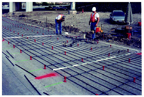
Figure 87. Instrumented section delineated by crack inducers.
RoctestTM embedment vibrating wire gages type EM-5 were installed on the instrumented area at three different depths at midslab, edge, and corner (150 mm from the crack). Type T thermocouples were also installed at seven different depths throughout the pavement depth. The thermocouple located at the PCC surface was installed just after the slip form paver passed by the instrumented area. In addition, resistance gages type CEA-06-125UN-120 were epoxied to the steel rebar at different distances from the expected crack along with embedment gages to monitor the steel and concrete strain. After adhering the gage, mechanical protection was applied to avoid damage of the gage during the construction operations. Figure 88 shows the strain gages in concrete and on the reinforcing steel at the corner location.
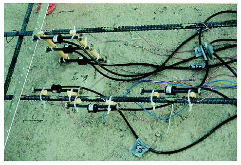
Figure 88. Strain gages in PCC and on reinforcing steel.
On the paving day, the instruments were doublechecked for position, elevation, and tightness. References were marked outside of the slab to determine the exact location of the instruments after the slabs were paved. Every detail in the construction operations was recorded. Shortly before the paver passed by the instrumented slab, the gages and thermocouples were protected with fresh concrete and vibrated with manual equipment. Testers ensured that the concrete used to protect the sensors was from the same batch to be used in the rest of the instrumented area. Some records from the placement activities are:
To measure CTE and free drying shrinkage in the field, two cylinder molds were instrumented with a vibrating wire strain gage and a thermocouple at the center of the specimen.
To ensure development of crack formation, green sawing was performed on the adjacent cracks to the instrumented area with Soff-Cut equipment approximately 2.5 hours after placement.
To measure the slab curling and warping, LVDTs were installed at the edge and at the corner of the test slab. These instruments were installed approximately 10 hours after placement and before the cracks had occurred.
After the concrete had set, DEMEC buttons were glued on the location of the crack inducers and 0.51 m toward the center of the slab along the edge from each crack. On the second day, after the first cracks appeared, DEMEC buttons were also glued at 20 additional cracks to monitor the crack movement due to temperature fluctuations and drying shrinkage.
A friction test also was performed to characterize the friction force developed at the concrete slab-subbase interface. The procedure consisted of casting a 0.9-m wide by 1.5-m long plain concrete slab, with the same thickness of the projected CRCP pavement, on top of the same subbase type. The slab was cast on July 13, 2001, and the friction test was performed 5 days later. For this test, a force was applied on one side of the slab with a hydraulic jack. A load cell was used to measure the applied load. Dial gages were installed at the opposite side to measure the slab movement. The friction force was determined from the applied load and the area under the slab. The history of friction force and slab movement during the pushoff procedure was recorded. The friction force at sliding also was identified. During the determination of the friction for this section, it was observed that the bond between concrete and asphalt was so strong that shear forces developed in the asphalt. This originated a plane of failure in the asphalt along the border of the slab against which the load was applied, as illustrated in figure 89. Both the concrete slab and bonded asphalt slid together, originating the friction force underneath the asphalt subbase, between the asphalt layer and the lime-treated subgrade.
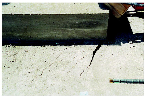
Figure 89. Shear failure as a result of pushoff test.
On the days following placement, pavement profiles were measured with Dipstick equipment to detect any changes in the profile of the CRCP slabs due to curling and warping. The pavement profiles were measured at several slab diagonals in between cracks at two different times during the day. The measurements were made early in the morning, when the pavement was at its coolest temperature at the surface, and in the afternoon, when the pavement surface had warmed up, to capture the maximum difference in shape of the CRCP slabs due to different thermal gradients. The climatic conditions at the site were monitored for the 72-hour period after placement. The air temperatures during the first days after construction ranged from 26.6 °C to 40.0 °C.
Dataloggers were used to constantly monitor the pavement. This equipment was programmed to retrieve concrete strains, concrete temperature, and vertical displacement every 10 minutes during the 72-hour period. Weather conditions were recorded every 15 minutes during the 72-hour period.
Condition surveys were performed for the entire section placed on July 16, 2001, to observe the cracking pattern in terms of crack spacing and crack width. During the same period, crack movement and PCC strain were monitored with DEMEC calipers twice a day.
During construction, the surface of the pavement was finished on two 76 by 76-mm squares 457 mm from the slab edge and separated 305 mm from each other, center to center. This was done to estimate the PCC set time with pulse velocity equipment. These areas were finished to leave a smooth surface. During monitoring of the test slab, the pulse velocity transducers were placed against both surfaces separated 305 mm apart, center to center, to obtain the transit time of the ultrasonic pulses traveling in the concrete from one transducer to the other. Although the reinforcing steel affected the pulse velocity measurements (resulting in an overestimation of the elastic modulus), the rate of change in pulse velocity with time provided a good indication of when set time occurred. Analysis of this information indicates that set time occurred at approximately 3 hours, which seems to correlate well with the high placement temperatures observed.
During the condition surveys, it was observed that a crack formed at the location of both crack inducers, as planned. The average crack spacing for the rest of the placement on that day was very close to the crack spacing observed in previous days. On the second and third day, additional cracks were observed at some areas with previously large crack spacings. However, for the instrumented section, no intermediate cracks were observed during the monitoring period. Figure 90 shows the sensor locations with respect to the observed cracks as constructed.
Figure 90. Position of strain gages and thermocouples as constructed.
Concrete specimens were prepared at the site with the same batch of concrete delivered on the instrumented section. Personnel with the FHWA Mobile Concrete Laboratory helped prepare the concrete specimens. The specimens were cured in the field for the first 24 hours, then cured under laboratory conditions according to ASTM C 192. While at the site, sufficient materials to replicate the concrete mix in the laboratory were collected. The materials collected were used to perform adiabatic calorimetry, drying shrinkage, and set time tests.
The second field section for the CRCP model validation was selected in the State of South Dakota. At the end of the summer of 2001, the South Dakota DOT was reconstructing I-29 south of Sioux Falls, SD, from approximately milepost 59 to milepost 70. In contrast to the CRCP instrumentation in Texas with air temperatures from 26.6 °C to 40.0 °C, the air temperatures in South Dakota ranged from 1 °C to 24.4 °C, providing a significant difference in terms of temperature and behavior under which the CRCP module will be evaluated and validated.
South Dakota DOT representatives and a member of the South Dakota Chapter of the American Concrete Pavement Association (ACPA) helped locate a CRCP construction job in South Dakota. Beginning on September 25, 2001, a section of CRCP pavement was instrumented and monitored for 72 hours. Once at the site, all the preconstruction information was collected, including pavement design, mix design, and materials. The typical cross section at the construction site on I-29 is designed to accommodate a four-lane divided road. Each direction is 12.2-m wide, with a 1.8-m left shoulder, two 3.65-m lanes, and a 3-m right shoulder as indicated in figure 91 (this figure shows the section in the opposite direction to traffic). The central portion of the pavement was being constructed with CRCP pavement to conform a 3.65-m wide right lane with 0.6-m PCC widened shoulder and a 3.65-m wide left lane. The rest of the shoulders were being paved with HMA. A longitudinal joint was being cut between lanes. The CRCP pavement is 279 mm thick on top of a 102-mm granular subbase.
1 ft = 0.3048 m
Figure 91. Typical cross section for I-29, South Dakota (from opposite direction to traffic).
To characterize the properties for the concrete at the site, information was collected on the mix design, admixtures, and additives used, as well as the coarse and fine aggregate properties and geological type. The mix design for this project is shown in table 66.
| Mix Design (Saturated Surface Dry) | kg/m3 |
|---|---|
| Water | 140 |
| Cement type I/II | 303 |
| Fly ash class F | 67 |
| Fine aggregate | 724 |
| Coarse aggregate, maximum aggregate size 25.4 mm, crushed ledge rock (Sioux quartzite) | 1043 |
| Water reducer-WRDA 82 | 774-1160 ml/m3, depending on weather conditions |
| Air entrainer-Daravair® R | 690 ml/m3 (6.5 percent air) |
The field crew arrived at the project the morning of September 24, 2001. After a briefing on the instrumentation procedures, the South Dakota DOT helped identify the section to instrument. The section that was placed on Friday, September 21, 2001, was surveyed to identify the average crack spacing. The crack spacing observed varied from 4.3 m to 18.3 m, with an average spacing of 9.1 m. This survey helped determine the location for the crack inducers on the instrumented section. The crack inducers thus were spaced at approximately 9.1 m.
Similar to the instrumentation of the CRCP section in Texas, embedment gages type EM-5 were installed at midslab, edge, and corner at three different depths. Thermocouples were also installed at seven different depths throughout the pavement. Micromeasurements CEA-06-125UN-120 gages were also installed on the steel rebars at different distances from the crack. In addition, similar procedures were used to monitor climatic conditions, CTE and free drying shrinkage in the field, slab curling and warping, and cracking behavior.
To position the Roctest vibrating wire gages type EM-5, two wood dowels were driven into the subbase (granular subbase), separated approximately 102 mm for each set of gages, as indicated in figure 92. The gage then was fixed on the dowels at the proper height with plastic zip ties. Wood dowels were also used to install type T thermocouples at seven different depths throughout the pavement. The thermocouple located at the PCC surface was installed just after the slip form paver passed by the instrumented area.
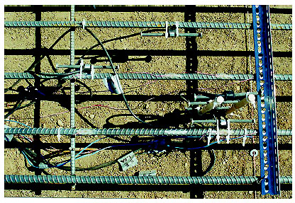
Figure 92. Strain gages in PCC and on reinforcing steel.
The procedure to install the micromeasurements CEA-06-125UN-120 steel gages consisted of grinding the rebar corrugations to leave a smooth surface. After the corrugations were ground, a file was used to smooth any surface indentations. The surface was smoothed even more with sandpaper grade 60, then with sandpaper grade 400. The grinding was done so as not to reduce the diameter of the rebar. Before adhering the resistance gage to the surface, isopropyl alcohol was used to clean and degrease the treated surface of the rebar. The gages with preattached lead wires were taped to the rebar. A conditioning solution was brushed on the surface of the rebar and on the area of the gage to be bonded to the rebar. After 1 minute of drying, M-bond 200TM adhesive was used to adhere the resistance gage to the rebar. After M-bond 200 was applied, the gage was held down against the surface of the rebar for at least 1 minute. After adhering the gage, researchers applied mechanical protection to avoid damage of the gage during the construction operations.
After all the gages were installed, a small trench was dug into the subbase on the area of the paver track to lead all the sensor wires out of the pavement and to the dataloggers.
Some records from the placement activities are:
As discussed previously, the crack spacing initially estimated for this section was approximately 9.1 m. However, the cooling cycle after placement reached a low temperature of 1 °C, which was beyond the forecasted low temperature of 4.4 °C. This excessive temperature drop significantly reduced the crack spacing, and one intermediate crack occurred at the instrumented section on the first day. On the second day, two additional cracks were observed (see figure 93). However, the additional cracks in the instrumented section did not affect the main objective of the experiment, which was to determine the development of concrete and steel strains near the crack locations. In addition, the data collected for this site complemented the data collected for the Fort Worth, TX, section, where no intermediate cracks were observed. Figure 94 shows the sensor locations with respect to the observed cracks as constructed.
Figure 93. Cracking pattern on instrumented section.
Figure 94. Location of the sensors with respect to the pavement edge and cracks as constructed.
Concrete specimens were prepared at the site. These specimens were prepared to characterize the concrete properties under laboratory and field conditions. Two sets of laboratory concrete specimens were prepared as described in table 67. The first was cured under field conditions according to ASTM C 31, and the second set was cured under laboratory conditions according to ASTM C 192. The difference in curing procedures was done to verify the maturity properties for this specific concrete.
| Test | Field Curing Conditions | Laboratory Curing Conditions |
|---|---|---|
| Splitting tensile | Three repetitions at 1, 2, and 3 days | Three repetitions at 1, 3, 7, and 28 days |
| Compression | - | Three repetitions at 3, 7, and 28 days |
| Modulus of elasticity | - | Three repetitions at 7 and 28 days |
| CTE | - | Two repetitions at 28 days |
| Temperature monitoring | One specimen | One specimen |
This appendix presents the laboratory testing data for the HIPERPAV II sites in Illinois, Mexico, South Dakota, and Texas. Laboratory testing included compressive strength, splitting tensile strength, modulus of elasticity, CTE, drying shrinkage, and set time. The testing matrix is provided in table 68.
| Site | Compressive Strength | Splitting Tensile Strength | Modulus of Elasticity | Drying Shrinkage | Set Time | CTE |
|---|---|---|---|---|---|---|
| Illinois | X | X | X | - | - | X |
| Mexico | X | X | X | - | - | X |
| South Dakota | X | X | X | X | X | X |
| Texas | X | X | X | X | X | X |
The laboratory results are presented in the sections below, as are the concrete mix designs.
The concrete mix designs for the sites in Illinois, Mexico, South Dakota, and Texas are given in table 69.
| Illinois | Mexico | South Dakota | Texas | |
|---|---|---|---|---|
| Cement type | I | I | II | IP |
| Cement content | 341 kg/m3 | 280 kg/m3 | 303 kg/m3 | 309 kg/m3 |
| Cementitious materials content | - | - | Fly ash class F 67 kg/m3 | - |
| Water content | 148 kg/m3 | 158 kg/m3 | 140 kg/m3 | 138 kg/m3 |
| Coarse aggregate content | 1121 kg/m3 | 1006 kg/m3 | 1043 kg/m3 | 1105 kg/m3 |
| Maximum aggregate size | - | 38.1 mm | 25.4 mm | 38.1 mm |
| Aggregate type | - | - | Sioux quartzite | Limestone |
| Fine aggregate content | 666 kg/m3 | 932 kg/m3 | 724 kg/m3 | 678 kg/m3 |
| Water reducer | Type A WRDA with Hycol | 1333 ml/m3 | WRDA 82 774-1160 ml/m3 |
HPS-R 1082 ml/m3 |
| Air entrainer | Darex® AEA | 115 ml/m3 | Daravair R 690 ml/m3 |
AIR-INTX 108 ml/m3 |
At the Fort Worth, TX, I-35 West/I-30 interchange, a 203-mm thick CRCP was constructed on July 16, 2001. More details on the highway construction are given in section C.2.1. Several cylinders were molded to measure concrete material properties at 0.5, 1, 3, 7, and 14 days. The concrete specimens were cured in the field for the first 24 hours and then under laboratory conditions according to ASTM C 192. The compressive strength, splitting tensile strength, and modulus of elasticity as a function of time are shown in figures 95 to 97. All specimens were soaked until the time of testing. The individual data points are hollow, and the average is shown as a solid point.
Figure 95. Time growth of Texas compressive strength.
Figure 96. Time growth of Texas splitting tensile strength.
Figure 97. Time growth of Texas modulus of elasticity.
Because the compressive strength was measured on 102-mm and 152-mm diameter cylinders, it had to be adjusted for the different cylinder sizes.(61) All the splitting tensile tests were completed on 152-mm cylinders. The compressive strength and the splitting tensile strengths continue to increase from 0.5 to 14 days. Variability of the splitting tensile strength is high at early ages.
The modulus of elasticity data do not increase with time. The modulus increases from 0.5 to 3 days, and then drops at 7 and 14 days. The FHWA Mobile Concrete Laboratory tested the early-age concrete (0.5 to 3 days), and Construction Materials Research Group at the University of Texas at Austin tested the 7- and 14-day samples. Variability in testing and data interpretation may have contributed to the difference in modulus values. Using the ACI correlations between compressive strength and concrete modulus of elasticity shown in equations 259 and 260:(58)
ACI 318 Code (1):
![]() (259)
(259)
and
ACI 318 Code (2):
 (260)
(260)
It is apparent that the expected modulus of elasticity value lies below the high values at early ages, and above the low values at 7 and 14 days. The raw laboratory data for the Texas site are given in tables 71 to 74 in sections C.8 to C.10.
The laboratory results for compressive strength, splitting tensile strength, and modulus of elasticity are presented here for the CRCP constructed in South Dakota on I-29. More details on the construction process and monitoring are provided in section C.2.2. It is apparent that the compressive strength, tensile strength, and modulus of elasticity increase with time in figures 98 to 100. Likewise, the modulus of elasticity for South Dakota is estimated from the compressive strength data using the ACI and ACI 318 models in figure 100. The model predictions are lower than the measured data.
Figure 98. Time growth of South Dakota compressive strength.
Figure 99. Time growth of South Dakota splitting tensile strength.
Figure 100. Time growth of South Dakota modulus of elasticity.
An extensive pavement evaluation was conducted on the JCP section of the Ticuman bypass on August 21-24, 2001. This pavement was originally constructed from September 23 to October 12, 1993. The early-age laboratory data from 1993 are compared to the properties measured in 2001 in the figures below (figures 101 to 103). The concrete strength continued to increase over time, as expected, as does the splitting tensile strength and the modulus of elasticity. The modulus of elasticity is estimated using the ACI and ACI 318 models in figure 103. The predicted values are in the same range as the measured ones.
Figure 101. Time growth of Mexico compressive strength.
Figure 102. Time growth of Mexico splitting tensile strength.
Figure 103. Time growth of Mexico modulus of elasticity.
U.S. Highway 50, a JPCP near Carlyle, IL, was monitored from August 7 to 10, 2001. It was originally constructed from April to August of 1986. At that time, air content was 5.4 percent, slump was 51 mm, the 14-day flexural strength was 4.9 MPa, and the 28-day flexural strength was 492 MPa. Cores of the pavement were taken and tested in May 2002. The resulting concrete properties are listed in table 70.
| Illinois | Concrete Properties (MPa) |
CV (%) |
|---|---|---|
| Compressive strength | 40.7 | 3.9 |
| Splitting tensile strength | 4.57 | 1.6 |
| Modulus of elasticity | 27,441 | 2.2 |
The flexural strength data, which are assumed to be measured under centerpoint loading, were also used to estimate the early-age compressive strength of this concrete using the relationship shown in equation 261:
 (261)
(261)
Its comparison to the compressive strength measured in May 2002 is shown in figure 104. After 14 days, the data show a minimal increase in compressive strength, except for the 90-day calculated value.
Figure 104. Time growth of Illinois compressive strength.
Likewise, the estimated compressive strength values are used to predict the modulus of elasticity (figure 105). They correlate well to the measured modulus of elasticity, except for the 90-day value as mentioned previously. Modulus of elasticity is relatively stable after 14 days.
Figure 105. Time growth of Illinois modulus of elasticity.
The drying shrinkage of the concrete placed in Fort Worth, TX, and South Dakota was measured in the laboratory using ASTM C 157, with minor modifications. The specimens were 102-mm prisms that were 286 mm long. The concrete mix quality control parameters are given in table 72. They were cured 24 hours at 100 percent RH and 23 °C, then were stored at 50 percent RH at 23 °C for the remaining period of time. Readings were taken every day for the first 7 days, and then at 14, 28, and 112 days. The time growth of drying shrinkage is shown in figure 106 for South Dakota and in figure 107 for Texas. The Baźant-Panula drying shrinkage model is fit to the laboratory data, as shown (described in section B.1.3). If the ultimate shrinkage is known, it can be input to the model, or the Baźant-Panula model can predict ultimate shrinkage. A more accurate prediction is made if the ultimate drying shrinkage is known.
Figure 106. Drying shrinkage of South Dakota concrete.
Figure 107. Drying shrinkage of Texas concrete.
The drying shrinkage input parameters for the Baźant-Panula model are listed in table 71. The concrete mix proportions that were input to the model were taken from table 69.
| Input | South Dakota | Texas |
|---|---|---|
| 28-day compressive strength (MPa) | 37.3 | 33.4 |
| 28-day modulus of elasticity (MPa) | 33,784 | 27,580 |
| Set time (days) | 0.28 | 0.20 |
| D (= 2 * volume/surface area) (mm) | 46 | 46 |
| ks | 1.28 | 1.28 |
| a1 | 0.85 | 1 |
| a2 | 1 | 1 |
The 28-day compressive strength and modulus of elasticity values were estimated from the measured laboratory data. Set time was taken from the data in the following section. Finally, ks, the shape parameter, represents the shape of the laboratory produced drying shrinkage specimens.
The set times for the concrete placed in Fort Worth, TX, and South Dakota were determined by following ASTM C 403. The quality control data for these mixes are given in table 72.
| Concrete Property | South Dakota | Texas |
|---|---|---|
| Slump | 45 mm | 70 mm |
| Batching temperature | 22.2° C | 21.7° C |
| Batching date | 10/26/2001 | 10/26/2001 |
| Batching time | 10:39 a.m. | 11:27 a.m. |
| Air content (%) | 4 | 5.5 |
| Unit weight (kg/m3) | 2340 | 2262 |
The set time data for Fort Worth, TX, were fit using a power function, with an r² of 0.99 (figure 108). The corresponding initial and final setting times are listed in table 73. The ambient temperature for measuring the Texas mix set time was 37.8 °C.
Using a regression analysis, the r² for the South Dakota data is 0.97. This is less than the 0.98 required by the specification for the set time analysis, so the data were hand fit, as shown in figure 108. The initial and final setting times are listed in table 73. The ambient temperature for the set time measurements using the South Dakota concrete was 18.3 °C.
Figure 108. Setting times of concrete for Texas and South Dakota concretes.
| Setting Time | Texas | South Dakota |
|---|---|---|
| Initial setting (min) | 242 | 304 |
| Final setting (min) | 292 | 396 |
The concrete and air temperatures for the fresh concrete mixes from South Dakota and Texas are shown in figures 109 and 110.
Figure 109. Concrete and ambient air temperatures for the South Dakota concrete.
Figure 110. Concrete and ambient air temperatures for the Texas concrete.
CTE tests were also performed on concrete specimens for each field site on June 6, 2002. AASHTO test method TP-60-00 was followed. The average CTE values obtained for the PCC specimens tested are listed in table 74.
| PCC Specimen ID | CTE (x 10-6 m/m/°C) |
|---|---|
| Fort Worth, TX | 7.48 |
| Illinois | 6.85 |
| Mexico | 7.00 |
| South Dakota | 10.91 |

