U.S. Department of Transportation
Federal Highway Administration
1200 New Jersey Avenue, SE
Washington, DC 20590
202-366-4000
Federal Highway Administration Research and Technology
Coordinating, Developing, and Delivering Highway Transportation Innovations
 |
| This report is an archived publication and may contain dated technical, contact, and link information |
|
Publication Number: FHWA-RD-98-155 Date: FEBRUARY 1999 |
This chapter provides a number of key concepts related to the current PRS approach that must be understood before attempting to use the revised PRS prototype. The chapter starts with a general discussion of pavement performance and how it is defined under the PRS approach. The specific step-by-step PRS procedure used to predict the performance of a given lot is presented. Next, the concept of computing and using the lot LCC as the overall measure of quality (for both the as-designed and as-constructed pavements) is explained. The step-by-step procedures used to compute an overall lot LCC are discussed. Finally, the procedures used to compute Level 1 and Level 2 pay adjustments (based on the estimated as-designed and as-constructed LCC's) are explained.
The underlying concept of PRS is that knowledgeable decisions related to pavement lot acceptance and corresponding pay adjustments are based on the predicted pavement performance. Under the current PRS approach, pavement performance is expressed in terms of different identified pavement distresses, referred to as distress indicators. In a previous PRS study, many distress indicators were identified that were not only assumed to have a significant effect on the service life of the pavement, but were also under the control of the contractor.(1) Based on each identified distress indicator's significance to concrete pavement performance and the availability of mathematical-based prediction models, the following four distress indicators were selected for inclusion in the original, and also the revised, prototype PRS:(1)
Although the chosen distress indicators are exclusively related to the concrete slab,
distress indicators related to other pavement components (such as the subgrade, base, and
shoulders) should eventually be included in more comprehensive PRS. The current PRS
methodology allows for the eventual inclusion of any number of distress indicators.
These four distress indicators included in the revised PRS are predicted
over a chosen analysis period using the best prediction models available.
These mathematical models are functions of a series of defined project-specific
constant values (e.g., traffic, climatic variables, design characteristics,
drainage and support conditions, project dimensions, and unit costs) and
relevant AQC sample means. The general inputs and outputs for each of
the available PRS distress indicator models are shown in figure 1.Each
distress indicator model is explained in detail in
appendix E (volume III).
Figure 1. Inputs and outputs of the distress indicator prediction models available in the revised PRS prototype.
Although pay adjustments are applied on a lot basis, pavement performance is predicted for each sublot under the current PRS approach. A sublot is a discrete amount of pavement (part of a lot) from which AQC's are measured. A chosen number of AQC samples are taken from each sublot and tested using agency-approved testing procedures. Note that the number of samples per sublot may differ for each AQC. The sublot means of the AQC testing values, and the project-specific constant values, are then used in the distress indicator models to predict the respective sublot distresses over time. This procedure is repeated for every sublot within a lot; therefore, the performance of the entire lot is defined in terms of the independently predicted sublot distresses. Because the predicted sublot distresses are dependent on the representative sublot AQC means, changes in the between-sublot quality level impact the predicted between-sublot performance. Figure 2 illustrates an example of the procedure used to predict the pavement performance of a given lot. (Note: The AQC sampling types and frequencies chosen for this example are for illustration purposes only.)
Figure 2. Process for predicting the pavement performance of a given lot (sample types and number of samples per sublot are for illustration purposes only).
A driving concept of the current PRS approach is that the predicted future LCC of a pavement lot is the overall quality characteristic used for determining contractor pay adjustments. The lot LCC can generally be defined as the cumulative PW value of the future pavement performance-related costs expected to be incurred by the SHA (and users, if so desired) over the chosen analysis period. This LCC definition is, of course, very much dependent on what specific types of costs the agency chooses to include. Under the current PRS approach, the agency may choose to consider not only expected M & R costs, but user costs as well. Each of the specific cost types available for inclusion are discussed in more detail below.
The costs incurred by the agency include all of the M &
R costs expected to be required to keep the pavement lot in service (at an acceptable
quality level) over the chosen analysis period. Rehabilitation costs are divided
into localized and global rehabilitation costs. Each of these agency-incurred cost
types is discussed separately below.
Maintenance costs are those costs associated with the
application of day-to-day maintenance activities performed to address safety and
operational concerns and prevent the rapid deterioration of the pavement structure.
These activities are generally referred to as preventive or routine
maintenance. This maintenance is typically applied at certain fixed intervals of
time over the life of a pavement lot (commonly on an annual basis). The current PRS
approach limits maintenance costs to those resulting from transverse crack and transverse
joint sealing.
Local rehabilitation costs are those resulting from the
application of localized rehabilitation activities (used to correct localized distresses).
Localized distresses are those that affect an individual joint (transverse joint
spalling and transverse joint faulting) or an individual slab (transverse slab cracking).
The current PRS approach considers costs resulting from the following local
rehabilitation activities:
Global rehabilitation costs are those costs resulting from activities applied to the entire pavement lot in response to declining global pavement conditions. These activities are specifically applied to address pavement conditions such as decreasing pavement smoothness, increasing amounts of localized distress, or increasing amounts of applied localized rehabilitation. These activities are referred to as global because they are applied to the entire lot (all sublots) at the same point in time (based on the consideration of the individual performance of all sublots within the lot). In the current PRS approach, global rehabilitation costs can be the result of AC overlays, PCC overlays, or diamond grinding.
The concept of having the contractor pay adjustment dependent on estimated future costs incurred by pavement users has long been debated when discussing PRS. User costs are defined as pavement condition-related costs incurred by the users of the facility over the chosen analysis period. The current PRS approach allows the consideration of the following four user cost types defined by McFarland and presented in a recent report discussing LCC's:(10,13)
The inclusion of user costs in the lot LCC's used to compute PRS pay adjustments continues to be a controversial issue. In response, the revised prototype PRS allows for the inclusion of a specified percentage of the estimated total user costs over the chosen analysis period. This percentage may be set equal to zero if an agency does not wish to include any user costs. The inclusion of user costs does, however, allow the SHA to emphasize the effects of pavement smoothness on LCC's and subsequent pay adjustments.
The calculation of the representative LCC for a given lot is
based on estimating all of the future maintenance, rehabilitation, and user costs (if
included) related to the predicted performance of the given lot. The performance of
the lot, defined in terms of sublot distresses versus time, is predicted using the
procedure outlined in figure 2. An
agency-defined M & R plan is applied to these streams of sublot distresses in order to
determine when and what type of M & R activities are expected to be applied.
Typically, a series of defined pavement conditions (individual distress levels,
combinations of distress levels, and limits on the number of applied localized repairs) is
used to trigger localized and global rehabilitation.
Following is the step-by-step procedure used to determine
the particular timing of M & R activities and their associated costs, which are, in
turn, summarized into a representative lot LCC.
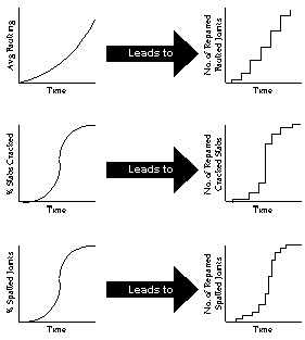 |
| Figure 3. Example of the relationships between the predicted distress indicators and the application of corresponding localized rehabilitation for a given sublot. |
The schedule of applied maintenance is slightly more complex, as it depends not only on the scheduled timing of the maintenance activities (defined in the M & R plan), but also on the amounts of the predicted localized distress. For example, as the total linear feet of predicted slab cracking increases, so does the amount of required crack sealing. Similarly, every transverse joint that is replaced to correct spalling results in two new joints (both sides of the new patch) that require sealing.
- Individual distress indicators—i.e., percent (or number) of cracked slabs, percent (or number) of spalled joints, and average faulting per joint.
- Combinations of individual distress indicators—e.g., apply global rehabilitation if percentage of cracked slabs = 20 percent and percentage of spalled joints = 30 percent.
- Applied levels of localized rehabilitation—e.g., apply global rehabilitation when a total of 20 percent of the transverse joints have been repaired for spalling.
Predicted distresses, and their corresponding required localized rehabilitation, are estimated each year over the progressing life of the pavement. The computed cumulative distresses, or localized rehabilitation, are then compared to the agency-defined lot threshold trigger values. When a computed cumulative distress or localized rehabilitation value surpasses a predefined lot threshold trigger value, the first global rehabilitation is triggered for application at that age.
An example of this lot threshold trigger value method is illustrated in figure 4. For this example, the agency has chosen to determine the timing of the first global rehabilitation based on two different lot threshold trigger values: (1) if the cumulative percentage of replaced slabs due to cracking equals 20 percent or (2) if the average sublot PSR equals 2.5. Both of these trigger values are checked each year over the progressing life of the pavement. For this particular example, it is the average sublot PSR that is the controlling criterion, since it reaches its respective trigger value at an earlier age than the percentage of cracked slabs. The average sublot PSR reaches a value of 2.5 at an age of 17.5 years, while the percentage of cracked slabs did not reach its trigger value of 20 percent until year 19.25. Therefore, the first global rehabilitation is scheduled to be applied to the lot (all sublots) at an age of 17.5 years.
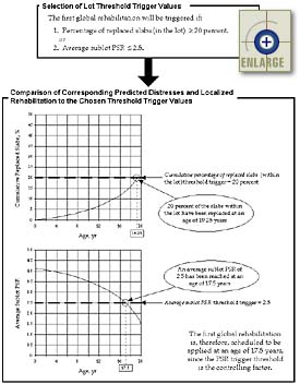 |
| Figure 4. Example of the lot threshold trigger method used to determine the timing of the first lot global rehabilitation. |
An example of this PSF method is illustrated in figure 5. For this example, the lot is made up of six sublots. The agency-defined PSF threshold value is 20 percent; therefore, this threshold value will be surpassed when two of six sublots are labeled as failed (33 percent > 20 percent). The independently determined sublot failure ages are shown for each sublot within the example lot. These sublot failure ages are then used to create a plot of PSF versus age. Based on the individually determined sublot failure ages and an agency-defined PSF threshold value of 20 percent, the first global rehabilitation is scheduled to be applied when the second sublot fails at an age of 19.50 years. It is strongly recommended that a trigger value of 10 to 30 PSF be used as the lot trigger value for determining global rehabilitation. This criterion is realistic and provides for a reasonable effect of variability on the LCC and pay adjustment.
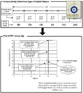 |
| Figure 5. Example of the PSF method used to determine the timing of the first lot global rehabilitation. |
Determine types and life spans of additional global rehabilitation applications.
After the timing of the first global rehabilitation is determined, the agency must
define the types and timings of additional global rehabilitation applications. Each
global rehabilitation activity is applied with an assumed life span (e.g., apply an AC
overlay with an assumed 15-year overlay life). Additional global rehabilitation
activities are then applied at the end of each assumed life span. (Note: Each
additional global rehabilitation does not have to be of the same activity type as the
preceding applied rehabilitation. For example, the agency could choose to apply
diamond grinding for the first and second global applications, and then follow those with
AC overlay applications until the end of the analysis period.) Global rehabilitation
activities may have different assumed life spans (e.g., an AC overlay may be assumed to
last 15 years, whereas diamond grinding may be assumed to last 8 years).
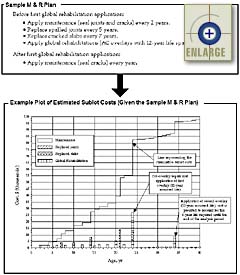 |
| Figure 6. Example showing the estimation of different M & R costs for one sublot (over the chosen analysis life). |
This entire lot LCC calculation process can be represented mathematically by the cost relationship shown in equation 7.
LCCLOT = S ALL SUBLOTS S YEARS [PW(MNT) + PW(LR) + PW(GR) + (A/100)*PW(UC)] (7)where
LCCLOT =Total present worth lot LCC, PW$.
PW(MNT) = Present worth of maintenance costs, PW$.
PW(LR) = Present worth of localized rehabilitation costs, PW$.
PW(GR) = Present worth of global rehabilitation costs, PW$.
A = Percentage of user costs to be included. (e.g., 3 percent is entered as 3).
PW(UC) = Present worth of user costs, PW$.
Pay adjustments under the revised prototype approach are based on a direct comparison of representative LCC's determined independently for both the as-designed and as-constructed pavement lots. Both as-designed and as-constructed representative lot LCC's are determined using the procedure described in the previous section.
Project-Specific Characteristics
The agency begins this comparison for a given project by defining and fixing those items that will not differ between the as-designed and as-constructed LCC determinations. These project-specific decisions include the following:
With all of these project-specific components held constant, the only variables that may differ between the as-designed and as-constructed pavements are the means and standard deviations of the chosen AQC's. Therefore, the difference between the resulting as-designed and as-constructed lot LCC's is the direct result of differences in the AQC quality.
Basic Pay Factor and Pay Adjustment Principles
The actual pay adjustment (incentive or disincentive) for a given lot is calculated as the difference between the as-designed LCC (LCCDES) and the as-constructed LCC (LCCCON). This pay adjustment may be expressed as a percentage of the representative contractor bid price for the given lot of concrete pavement. This relationship to the bid price is termed the pay factor (see equation 3).
Simulation of the Representative As-Designed Lot LCC
The representative as-designed lot LCC is simulated using the PaveSpec 2.0 computer software. As-designed target AQC means and standard deviations are selected by the agency and used to define the agency-desired pavement quality. If the as-constructed pavement is found to exactly match this desired quality (based on conducted AQC acceptance sampling and testing), the contractor will receive 100 percent of the submitted bid price (on average). The PaveSpec 2.0 software is used to simulate AQC sample sets (from the target AQC distributions) for N as-designed pavement lots. Each of the N simulated AQC sample sets results in the calculation of one possible LCC representing the as-designed target lot. The overall representative as-designed target LCC is, therefore, computed as the average of the N simulated lot LCC's. This process is illustrated in figure 7.
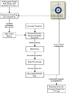 |
| Figure 7. Flow chart showing the process used to simulate the representative as-designed lot LCC (LCCDES). |
Simulation of the Level 1 Individual AQC Pay Factor Curves
The data flow process used to compute the LCC for any one
as-constructed lot is exactly the same as that used to compute the LCC for any one target
as-designed simulated lot. As mentioned previously, the same constant variables,
distress indicator models, acceptance sampling and testing plan, M & R plan, and cost
models are used for both the as-designed and as-constructed lot simulations. The
only difference between the procedures involves the AQC means and standard deviations used
to define the quality of the as-designed and as-constructed pavement lots.
If a Level 1 pay adjustment approach is chosen, independent
pay factor charts and corresponding equations are developed for each AQC. These pay
factor charts are developed prior to the bidding on the project and are made available to
the contractor. Hypothetical combinations of individual AQC means and standard
deviations are selected and assumed to be equal to the as-constructed pavement lot
quality. For each hypothetical combination, a representative as-constructed LCC is
simulated using exactly the same procedure used for the simulation of the representative
as-designed lot LCC (i.e., N AQC sample sets are simulated, resulting in N computed lot
LCC's—the representative as-constructed lot LCC is computed as the mean of the N
simulated as-constructed LCC values). Pay factors associated with each
representative as-constructed LCC (hypothetical combination of AQC mean and standard
deviation) are then determined using equation 3.
(Note: Since these curves must be made available prior to accepting contractor bids, a
representative bid price is used to compute the pay factors making up these curves [see
the section titled Selecting
an Appropriate Bid Price for Developing Level 1 Preconstruction Output in chapter
5, for more information]). Individual pay factor curves are constructed for specific
levels of AQC standard deviation (chosen by the agency), and over a chosen range of AQC
means, using the simulated representative as-constructed LCC's. Best-fit
regression equations are then determined, representing the data making up the individual
AQC pay factor curves. An example of a Level 1 pay factor chart for concrete
strength is shown in figure 8.
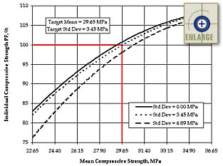 |
| Figure 8. Example of an individual Level 1 pay factor chart for concrete strength. |
It is important to emphasize that only one AQC is allowed to vary at a time when developing these Level 1 AQC pay factor curves. For example, when representative pay factors are being simulated for the individual concrete strength pay factor chart, all simulated pay factors (from hypothetical combinations of concrete strength mean and standard deviation) are determined with the other AQC means and standard deviations (for slab thickness, air content, initial smoothness, and percent consolidation) set equal to their target values. Figure 9 contains a flow chart showing the general simulation process used to develop Level 1 AQC pay factor curves and corresponding pay factor regression equations. A more detailed step-by-step procedure for generating these Level 1 AQC pay factor curves and corresponding pay factor regression equations is presented in chapter 7.
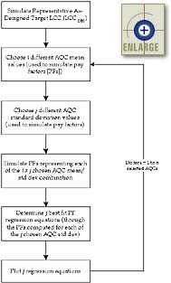 |
| Figure 9. Flow chart showing the process used to develop Level 1 AQC pay factor charts and corresponding equations. |
Level 1 Composite Pay Factors
After the construction of an actual pavement lot, the agency
takes samples from the pavement in accordance with the chosen acceptance sampling and
testing plan. The AQC sampling and testing values measured in the field (for the
given lot) are summarized into representative lot AQC means and standard deviations.
The lot means and standard deviations are then used in the individual AQC pay
factor regression equations to determine the corresponding independent AQC pay factors.
The procedure used to determine individual AQC Level 1 pay factors from the pay
factor charts is described in more detail in chapter
7.
Finally, the overall representative as-constructed Level 1
lot pay factor is determined by combining the individually calculated AQC pay factors into
one CPF representing the lot. The CPF equation essentially provides the appropriate
weighting factors for each independently determined AQC pay factor. This specific
CPF function is determined by the agency. A more detailed discussion of the commonly
used CPF equations is contained in chapter 6
in the section titled Defining a
Level 1 Composite Pay Factor Equation. Figure 10 contains a flow chart
showing the general process used to compute a Level 1 lot CPF.
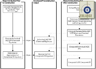 |
| Figure 10. Flow chart showing the process used to determine a Level 1 lot composite pay factor. |
The Level 2 pay adjustment does not require the use of a CPF equation. The lot pay factor is directly computed through simulation with the PaveSpec 2.0 software. After the placement of the as-construction pavement lot, samples are taken from each sublot according to the agency-chosen acceptance sampling and testing plan. Each set of AQC sublot samples is then statistically summarized to obtain AQC means representing each sublot. The sublot means are used in the chosen distress indicators to predict sublot performance, predicted sublot M & R activities, and their associated sublot LCC's. Finally, these sublot LCC's are summarized into one representative lot present worth LCC. The overall as-constructed lot pay adjustment and pay factor are then determined using this calculated as-constructed lot LCC in equations 1 and 2, respectively. Figure 11 contains a flow chart showing the general simulation process used to calculate a Level 2 lot pay factor.
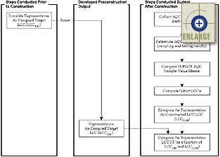 |
| Figure 11. Flow chart showing the process used to determine a Level 2 lot pay factor. |
Major Differences Between Level 1 and Level 2 Pay Adjustment Procedures
Three of the primary differences between the Level 1 and 2 pay adjustment procedures include the following:
It is important to emphasize that the Level 1 lot CPF is actually an estimate of the computed Level 2 lot pay factor. The Level 2 approach represents a simulated construction, sampling, testing, performance, and M & R over many years. Level 1 is a simplified method used to estimate the same pay factor as determined in Level 2, using more conventional pay factor curves.
Operating characteristic (OC) curves must be generated by the agency to determine if the chosen acceptance plan will perform as intended. The OC curves used with the PRS approach are similar to those used for conventional accept/reject acceptance plans, except that a set of OC curves is needed to reflect different payment options.(15) An example of the OC curves, commonly constructed for adjustable payment acceptance plans using actual lot percent defective procedures, is illustrated in figure 12. Each set of OC curves is specific to a chosen sampling plan (i.e., number of sublots per lot, number of AQC samples per sublot, and types of AQC samples and tests). The development of these curves is an integral part of the specification development process in that they provide the agency and the contractor with information regarding their respective risk. Similar OC curves can be developed for Level 1 specifications using the PaveSpec 2.0 computer software. The OC curves developed under the PRS approach are plots of probability of acceptance at the pay level specified versus AQC mean (rather than percent defective). More detailed information regarding the development of these curves using PaveSpec 2.0 is contained in chapter 7 in the section titled Developing Operating Characteristic Curves.
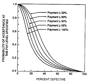 |
| Figure 12. Example of typical OC curves for an adjustable payment acceptance plan.(15) |