Volume 1: Practical Guide, Final Report and Appendix A

 

Introduction

After the agency makes all of the decisions required to develop a project-specific PRS, the final step required before actually using the specification is the generation of the appropriate preconstruction output. This chapter is provided as a step-by-step guide to generating preconstruction output for both Level 1 and Level 2 specifications.

 

Identifying Required Inputs

A number of steps are the same whether the agency chooses a Level 1 or Level 2 pay adjustment procedure. These steps require the collection of much project-specific information required to conduct LCC simulations. The specific steps for identifying the required inputs are detailed below.

Step 1—Define the General Project Information. The general project information should be identified as a first step. This information includes items such as project location, lane configuration, starting and ending stations, and lane widths. These are selected in accordance with the guidelines presented in the section titled Design-Related Variables, in chapter 5 of this volume.

Step 2—Define Pavement Performance. The agency must select the distress indicators that will be used to define pavement performance. These are selected in accordance with the guidelines presented in the section titled Defining Pavement Performance, in chapter 5 of this volume.

Step 3—Select the AQC's to be Included in the Specification. The agency must select the AQC's that are to be sampled and tested for acceptance. These are selected in accordance with the guidelines presented in the section titled Selection of Included AQC's, in chapter 5 of this volume.

Step 4—Define the Required Constant Values. A number of design-, climatic-, and traffic- related variables must be defined for use in the chosen distress indicator models. These are selected in accordance with the guidelines presented in the section titled Identification of Constant Variable Values, in chapter 5 of this volume.

Step 5—Define the AQC Acceptance Sampling and Testing Plan. The agency must define the sampling and testing procedures to be used in measuring the AQC's in the field. This plan not only defines the actual required sampling and testing methods to be used, but also defines the number of samples per sublot, the methods for determining random sampling locations, and some general information on retesting. The defined acceptance sampling and testing plan is determined in accordance with the guidelines presented in the section titled Selecting an AQC Acceptance Sampling and Testing Plan, in chapter 5 of this volume.

Step 6—Define the Required As-Designed AQC Target Values. The agency must select as-designed target means and standard deviations for each of the included AQC's. (Note: The selected means and standard deviations are dependent on the selected sampling and testing plan—defined in step 5.) Guidelines for selecting appropriate target values (interpreting existing specifications or from historical AQC construction data) are presented in the section titled Selection of AQC Target Values, in chapter 5 of this volume.

Step 7—Define Lots and Sublots. Lots and sublots must be clearly defined for the project. This primarily consists of defining the target lengths of each. The definitions for both lots and sublots are determined in accordance with the guidelines presented in the section titled Definition of Lots and Sublots, in chapter 5 of this volume.

Step 8—Define the Maintenance and Rehabilitation Plan. The agency must select an appropriate M & R plan to be used for the specific project. This involves selecting the type and frequency of application for maintenance, localized rehabilitation, and global rehabilitation activities. The defined M & R plan is determined in accordance with the guidelines presented in the section titled Selecting a Maintenance and Rehabilitation Plan, in chapter 5 of this volume.

Step 9—Define the Included Costs. The agency must identify the particular costs to be included in the overall lot LCC. These decisions include identifying the M & R unit costs associated with the chosen M & R activities, deciding on an appropriate percentage of user costs to be included, and determining an appropriate discount rate. All of these cost-related decisions are made in accordance with the guidelines presented in the section titled Cost-Related Decisions, in chapter 5 of this volume.

Step 10—Define the Simulation Parameters. In order to conduct any LCC simulations for the as-designed or as-constructed pavement, the agency must define the required simulation parameters, such as the number of simulation lots required to simulate a lot LCC and the appropriate range of number of sublots per lot. These simulation-related parameters are determined in accordance with the guidelines presented in the section titled Selecting Simulation Parameters, in chapter 5 of this volume.

Step 11—Choose the Appropriate Pay Adjustment Procedure. The agency must select one of two pay adjustment methods available in the prototype PRS—Level 1 or Level 2. Level 1 should be selected for initial implementation of PRS. This decision is made in accordance with the guidelines presented in the section titled Selecting a Pay Adjustment Procedure (Level 1 or Level 2), in chapter 6 of this volume. The details for each of these pay adjustment methods are explained separately in the following sections.  

Level 1—Generating Individual AQC Pay Factor Curves

For the Level 1 specification, the preconstruction output involves simulating data points making up the individual AQC pay factor charts. Each AQC pay factor chart is made up of a series of pay factor curves (each specific to a different AQC standard deviation) plotted over a chosen AQC mean range. Pay factor regression equations are fit through the data making up each pay factor curve. Individual AQC pay factors may then be determined using the developed regression equations (or read directly from these charts) by knowing the as-constructed AQC lot means and standard deviations. If the measured AQC standard deviation does not exactly match that of one of the simulated pay factor curves, the pay factor is determined by interpolating between the appropriate pay factor equations. An explanation of the development of the Level 1 pay factor curves (and corresponding pay factor regression equations) is contained in more detail in this section.

Level 1, Step 12—Simulate the As-Designed LCC. In order to calculate pay factors for different hypothetical levels of as-constructed AQC quality, the representative target as-designed LCC must first be simulated. The PaveSpec 2.0 specification simulation software is used to estimate representative target as-designed LCC's for the different numbers of sublots per lot chosen by the agency (see the section titled Selecting Simulation Parameters, in chapter 5 of this volume). For example, the agency may decide to simulate as-designed LCC's for three different scenarios where the number of sublots per lot would equal 3, 4, and 5. Each of these simulated LCC's (representing a specific number of sublots per lot) is a function of many different agency-defined variables, including the number of simulation lots, acceptance and sampling plan, M & R plan, AQC target values, analysis life, and chosen costs. Individual Level 1 pay factor charts will be developed independently for each scenario chosen by the agency.

Level 1, Step 13—Choose a Range of As-Constructed Means for Each AQC. Reasonable ranges of AQC means are selected that will define the values used in the simulation of the Level 1 AQC pay factor curves. These chosen ranges of AQC simulation means are based on the chosen AQC target values. The agency is required to define the range of the AQC means and the number of simulation points within the range. The agency-chosen values will be used to define the x-axis range of the developed Level 1 pay factor charts. It is recommended that the boundary conditions of this range be defined as the agency-defined AQC RQL's and MQL's (see the section titled Retesting Procedures in chapter 5 of this volume).

Level 1, Step 14—Choose a Range of As-Constructed Standard Deviation Levels for Each AQC. The pay factor curves (contained in the Level 1 pay factor charts) depend not only on the as-constructed AQC mean, but also on the as-constructed AQC standard deviation. Therefore, it is important to choose a range of as-constructed standard deviation levels that will show the influence of the AQC variability. Three to five different levels of standard deviation are typically chosen for each AQC. (One of the chosen standard deviation levels should always be the AQC target standard deviation.)

Level 1, Step 15—Simulate As-Constructed LCC's and Calculate an Independent AQC Pay Factor for Each Hypothetical As-Constructed Mean/ Standard Deviation Pair. The hypothetical as-constructed mean/standard deviation pair values (coming from combinations of means and standard deviations defined in Level 1, steps 13 and 14, respectively) are used to define individual simulation sessions in PaveSpec. Each AQC is investigated independently for each simulation session (e.g., if strength is being investigated, all of the other AQC as-constructed means and standard deviations are set equal to the target values). Each mean/standard deviation pair is used in PaveSpec to simulate a corresponding representative as-constructed LCC mean (AC-LCC_MEAN). A pay factor is calculated for each hypothetical pair using equation 3 in chapter 3 of this volume. (Note: Pay factors are calculated using an agency-selected appropriate bid price determined in accordance with the guidelines set forth in the section titled Selecting an Appropriate Bid Price for Developing Level 1 Preconstruction Output in chapter 5.)

Level 1, Step 16—Determine Individual AQC Pay Factor Regression Equations. Best fit regression equations are defined for each set of simulated pay factors related to each as-constructed AQC standard deviation (chosen in Level 1, step 14). These individual pay factor equations are generated using the PaveSpec 2.0 software.

Level 1, Step 17—Plot Pay-Factor Equations vs. AQC Mean. The defined pay factor regression equations (determined in Level 1, step 16) can be graphed easily as a function of the AQC mean. Pay factor charts (containing plots of all of the regression equations defined in Level 1, step 16) are then plotted for each AQC independently. These charts are created for each number of sublots per lot chosen by the agency (see the section titled Selecting Simulation Parameters in chapter 5 of this volume).

Level 1, Step 18—Define the CPF Equation. The agency must define a governing CPF equation in accordance with the guidelines presented in the section titled Defining a Level 1 Composite Pay Factor Equation, in chapter 6 of this volume.

Level 1, Step 19—Define Pay Factor Limits. The agency must define pay factor limits that are applied to the computed individual AQC pay factors, or the lot CPF, or both. Any chosen pay factor limits are determined in accordance with the guidelines presented in the section titled Selecting Pay Factor Limits, in chapter 6 of this volume.  

Level 2—Simulating the As-Designed LCC

For a Level 2 specification, the preconstruction output only involves the simulation of the target as-designed life-cycle cost (LCC_DES). Overall lot pay factors are calculated directly as a function of this LCC_DES, the determined as-constructed LCC (LCC_CON), and the contract bid price (using equation 3 in chapter 3 of this volume). This Level 2 LCC_DES is determined using the same procedure described in Level 1, Step 12.

 

Developing Operating Characteristic Curves

Under the Level 1 PRS, operating characteristic (OC) curves are generated for each AQC using the PaveSpec 2.0 computer software. Each set of OC curves is developed specific to a defined sampling plan (i.e., number of sublots, number of samples per sublot, and sample and test types). The following steps outline the general procedure used within the software to generate these charts:

For each AQC, the following applies:

1. Distributions of pay factors for different AQC mean values (over the chosen range of AQC means) are simulated by setting the as-constructed AQC standard deviation equal to the target value. Each distribution is the result of a minimum of 500 simulated lot pay factors.
   
   
2. Pay factor means and standard deviations (computed at each hypothetically chosen AQC mean) are plotted over the chosen range of AQC means. Relationships of pay factor mean and pay factor standard deviation versus AQC mean are determined. Figures 20 and 21 illustrate these respective relationships for slab thickness on an example project. Figure 20 is commonly referred to as an expected pay (EP) curve.
   
   
3. The user must define the different pay factor acceptance levels for which the probability of acceptance will be investigated (e.g., PF ³ 80%, PF ³ 100%, PF ³ 110%).
   
   
4. Finally, OC curves for each of the chosen pay factor acceptance levels are plotted using the results of steps 1 through 3. Figure 22 contains the example OC chart plotted using the relationships determined for the slab thickness example (determined in step 2).
   
   

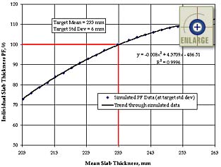Figure 20. Example of a simulated pay factor mean versus AQC mean relationship used to develop OC curves for a Level 1 PRS.

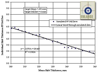Figure 21. Example of a simulated pay factor standard deviation versus AQC mean relationship used to develop OC curves for a Level 1 PRS.

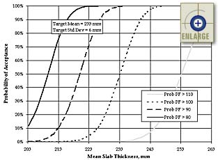Figure 22. Example of an OC curve constructed for a Level 1 PRS—case of four sublots and two samples per sublot (for each AQC). This chart reflects the relationships presented in figures 20 and 21.

Different examples of interpreting figure 22 are given as the following:

• If the contractor wishes to have a 50-percent probability that he/she will obtain a PF ³ 100 percent, then a mean slab thickness of 233 mm must be constructed.
  
  
• If the contractor wishes to have a 90-percent probability that he/she will obtain a PF ³ 100 percent, then a mean slab thickness of 240 mm must be constructed.
  
  
• If the contractor wishes to have a 90-percent probability that he/she will obtain a PF ³ 110 percent, then a mean slab thickness of 260 mm must be constructed.
  
  
• f the contractor actually builds a mean slab thickness of 223 mm (the target was 233 mm), the probability that he/she will receive a PF ³ 100 percent is approximately 5 percent. The probability that he/she will receive a PF ³ 90 percent is 70 percent.