U.S. Department of Transportation
Federal Highway Administration
1200 New Jersey Avenue, SE
Washington, DC 20590
202-366-4000
Federal Highway Administration Research and Technology
Coordinating, Developing, and Delivering Highway Transportation Innovations
 |
| This report is an archived publication and may contain dated technical, contact, and link information |
|
Publication Number: FHWA-RD-99-059 Date: FEBRUARY 1999 |
In PaveSpec, a project-specific PRS is created or edited using the Specification Wizard. This feature is comprised of 11 sequential steps (dialogue boxes) that lead the user through all aspects of developing a PRS-based specification. This chapter contains detailed descriptions of each dialogue box in the Wizard, as well as instructions on how to use them. The chapter ends with an explanation of the output report produced at the completion of the Specification Wizard steps.
Each dialogue box included in the Specification Wizard is equipped with four control buttons. The buttons may be activated by clicking on the selected button. The specific function of each of these buttons is described below:
| Allows the user to save the current specification document and return to the PaveSpec main window. (Note: A specification document can only be saved after all of the Specification Wizard steps have been completed.) | |
| Allows the user to quit the current specification development procedure (without saving changes) and return to the PaveSpec main window. | |
| Moves backward to the previous dialogue box in the Specification Wizard. | |
| Moves forward to the next dialogue box in the Specification Wizard. |
Whenever you choose to set up a new or previously developed specification, PaveSpec will start the Specification Wizard, and the Basic Specification Information dialogue box will appear. This dialogue box allows you to name the current specification, choose the type of specification to be developed (Level 1 or Level 2), and enter general descriptive project information. An example of this dialogue box is presented as figure 5.
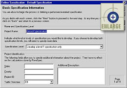 |
Figure 5.
Basic Specification Information dialogue box. |
To change the name of the current specification, type a new name in the Project Name input box. The name you enter will show up as the specification document name in the Specifications tab of the Database Control dialogue box.
The specification type must also be selected within this dialogue box. Currently, the user may choose to develop only a Level 1 specification or both Level 1 and Level 2 specifications at the same time. When defining specifications, the data required (and, therefore, the data input screens) vary depending on what specification type is selected. Any such differences will be explained in this chapter.
There are five different inputs grouped under the Project Identification heading. The data entered or selected in these fields are optional. These fields are included to allow the user to document descriptive information about the project to which the developed specification applies. Specific input fields include State, County, Project ID, Traffic Direction, and Additional Description. (The Additional Description input box is a notepad where you may enter any additional project information.)
Inputs used to describe the project’s lane configuration, location, and length are contained in the Dimensions and Lane Configuration dialogue box. An example of this dialogue box is presented in figure 6.
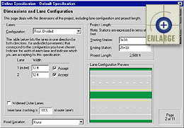 |
Figure 6.
Dimensions and Lane Configuration dialogue box. |
Choose the appropriate lane configuration describing the project’s layout from the Configuration drop-down box. The lane configuration is expressed as a combination of the total number of lanes making up the road (both traffic directions) and whether traffic (going in opposite directions) is divided by a median or barrier. The following six lane configurations are available to the PaveSpec user:
Note that the number of lanes being accepted at one time using the PRS is independent of the chosen lane configuration. For example, the lane configuration could be a six-lane divided highway; however, you may only be accepting (computing pay factors for) two lanes of paving.
Next, you must select the specific lanes that you would like to accept at one time using this specification. Select or deselect lanes by clicking on the Accept check box next to the lane of interest. For those lanes chosen for acceptance, lane widths must be entered in terms of either feet or meters (e.g., "12 ft" or "3.66 m"). (Note: You may toggle between English and metric units within any numerical input box using the " ` " key on your keyboard.) If an outer lane (lane adjacent to a shoulder) is chosen for acceptance and it is defined as a widened lane, select Widened Outer Lanes by clicking on that check box. To deselect the check box, simply click on the box again, and the "x" will disappear.
If you choose to accept an outer lane and an inner lane at the same time, you will need to specify the amount of inner lane cracking as a percentage of the predicted outer lane cracking. For example, if you select this number to be 100%, it will be assumed that all inner lanes being accepted will develop the same amount of cracking predicted for the outer lane. Conversely, if you select this number to be 0%, it will be assumed that all inner lanes being accepted will exhibit no cracking.
Select whether the project is located in an urban or rural setting by choosing the appropriate item in the Road Location drop-down box.
Lane Configuration Preview Window
The Lane Configuration Preview window provides an illustration of the type of lane configuration selected. Selecting a different item from the Configuration list box will change the contents of this preview window.
The starting and ending stations (expressed in ft or m) are also inputs in this Dimensions and Lane Configuration dialogue box. The specified station values are used to compute the total project length shown below the station input boxes.
The design-related variables used in defining a specification are grouped into three module documents. Not only does this simplify the logic of the process, but it also allows you to save and reuse groups of variables, which, in turn, simplifies the data entry itself. An example of the Design-Related Modules dialogue box is presented in figure 7.
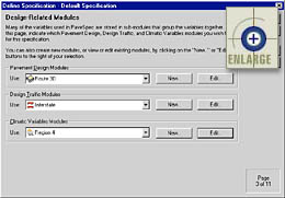 |
Figure 7. Design-Related Modules dialogue box. |
You
may access existing modules by clicking on the appropriate drop-down arrow
and highlighting the module you wish to use. To make changes to
a displayed module, click the ![]() button associated with that module type.
To create a new module, click on the
button associated with that module type.
To create a new module, click on the ![]() button. Whether
you decide to edit an existing module or create a new one, the data entry
screens will be the same—only the displayed input values will be
different. The data entry procedures for each module type will be
discussed separately.
button. Whether
you decide to edit an existing module or create a new one, the data entry
screens will be the same—only the displayed input values will be
different. The data entry procedures for each module type will be
discussed separately.
An example of the dialogue box used to define a Pavement Design module is presented in figure 8.
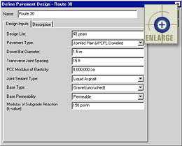 |
Figure 8.
Pavement Design Module dialogue box. |
The Pavement Design dialogue box is made up of two tabs: Design Inputs and Description. By default, the Design Inputs tab is displayed when you first enter the Pavement Design dialogue box.
All of the modules defining user inputs are contained in the Design Inputs tab. You can change the name of the Pavement Design module by entering a new name in the Name box. This name will then show up as the specification document name in the Modules tab of the Database Control dialogue box. The remaining design-related inputs in the Design tab are defined by entering appropriate values.
When entering data into the input boxes, the program presents the default units in English or metric depending on what Preferred Units type is selected in the program preferences. You may toggle between English and metric units within any numerical input box using the " ` " key. The following default units are used for both preferred unit types:
The Description tab contains a text box in which you may enter any detailed text describing the defined Pavement Design module. It is important to note that information entered in this text box is not used in the simulation process; therefore, it is optional.
Once
you are finished making changes or defining a Pavement Design module,
click on the ![]() button. If you would
like to exit the Pavement Design dialogue box without saving your
changes, click on the
button. If you would
like to exit the Pavement Design dialogue box without saving your
changes, click on the ![]() button. Clicking either button will return
you to the Design-Related Modules dialogue box.
button. Clicking either button will return
you to the Design-Related Modules dialogue box.
An example of the dialogue box used to define a Design Traffic module is presented in figure 9.
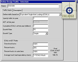 |
Figure 9.
Design Traffic Module dialogue box. |
The Design Traffic dialogue box includes two tabs: Traffic Inputs and Description. By default, the Traffic Inputs tab is displayed when you first enter the Design Traffic dialogue box.
All inputs used to compute yearly ESAL’s are contained in the Traffic Inputs tab. This dialogue box acts as a traffic calculator, allowing you to compute traffic over time based on an entered cumulative design ESAL or ADT at a specified year, a defined growth rate, and a chosen growth type (simple or compound). The relationship between ESAL’s and ADT is determined using the inputs defined in the ESAL-to-ADT Ratio section of the dialogue box. Cumulative ESAL’s are required by many of the distress indicator models, while yearly ADT values are used in the computation of any included user costs.
You can change the name of the Design Traffic module by entering a new name in the Name input box. This name will then show up as the specification document name in the Modules tab of the Database Control dialogue box. The remaining traffic-related inputs in the Traffic Inputs tab are defined by entering appropriate values.
The Description tab contains a text box in which you may enter any detailed text describing the defined Design Traffic module. Any information entered in this text box is optional, as it is not used in the simulation process.
Once
you are finished making changes or defining a Design Traffic module,
click on the ![]() button. If you would
like to exit the Design Traffic dialogue box without saving your
changes, click on the
button. If you would
like to exit the Design Traffic dialogue box without saving your
changes, click on the ![]() button. Clicking either button will return
you to the Design-Related Modules dialogue box.
button. Clicking either button will return
you to the Design-Related Modules dialogue box.
An example of the dialogue box used to define a Climatic Variables module is presented in figure 10.
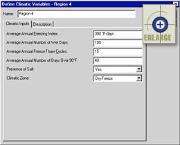 |
Figure 10. Climatic Variables Module dialogue box. |
The Climatic Variables dialogue box is made up of two tabs: Climatic Inputs and Description. By default, the Climatic Inputs tab is displayed when you first enter the Climatic Variables dialogue box.
All of the modules defining user inputs are contained in the Climatic Inputs tab. You may change the name of the Climatic Variables module by entering a new name in the Name input box. This name will then show up as the specification document name in the Modules tab of the Database Control dialogue box. The remaining climatic-related inputs in the Climatic Inputs tab are defined by entering appropriate values. For more information concerning the definitions and units of these variables, please see the section titled Climatic Variables in volume I.
The Description tab contains a text box in which you may enter any detailed text describing the Climatic Variables module. Because information entered in this text box is not used in the simulation process, it is optional.
Once
you are finished making changes or defining a Climatic Variables
module, click on the ![]() button. If you would
like to exit the Climatic Variables dialogue box without saving
your changes, click on the
button. If you would
like to exit the Climatic Variables dialogue box without saving
your changes, click on the ![]() button. Clicking either button will return
you to the Design-Related Modules dialogue box.
button. Clicking either button will return
you to the Design-Related Modules dialogue box.
Pavement performance is defined in page 4 of the Specification Wizard. An example of the Definition of Pavement Performance dialogue box is presented in figure 11.
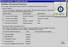 |
Figure 11.
Definition of Pavement Performance dialogue box. |
Pavement performance is expressed in terms of one or more of the four distress indicators (transverse joint faulting, transverse joint spalling, transverse slab cracking, and decreasing smoothness) shown in the Distress Indicators box. To select or deselect a distress indicator, click on the check boxes next to the distress indicators (a check mark signifies that the distress indicator is selected). For your convenience, the required and optional AQC’s associated with each distress indicator model are listed.
The second step in defining pavement performance requires the selection of AQC’s that you choose to measure in the field. The Status column next to the listed AQC’s indicates whether each AQC is Required, Optional, or Unnecessary. Those AQC’s required by the selected distress indicator models are automatically selected for inclusion (the corresponding check box is checked and the Status is shown as Required). Those AQC’s that are optional may be selected or deselected by clicking on the check boxes. AQC’s not required by the selected distress indicator models are automatically deselected (the corresponding check box is un-checked and the Status is shown as Unnecessary). If you choose to deselect an AQC that is required by one of the chosen distress indicator models, you will be asked to enter a model default value that will be used by those performance models requiring a value for that AQC.
The AQC sampling and testing plans are defined in page 5 of the Specification Wizard. You will see a tab for each AQC that you selected in the previous dialogue. Each AQC data entry screen is discussed separately.
This
AQC has two different data entry screens—one for sampling
information and one for testing information. If you chose
to develop a level 1 specification only, you can toggle between the level
1 sampling and testing data entry screens using the ![]() and
and ![]() buttons. If you chose to develop a level
1 and level 2 specification at the same time, you can also toggle between
the level 2 sampling and testing data entry screens using the
buttons. If you chose to develop a level
1 and level 2 specification at the same time, you can also toggle between
the level 2 sampling and testing data entry screens using the ![]() and
and ![]() buttons. (Note: The level 1 and level
2 sampling data entry screens are identical, as are the level 1 and level
2 testing data entry screens. Separate data entry screens are provided
for each PRS level only because you can choose to use different sampling
and testing plans for the different specification levels.)
buttons. (Note: The level 1 and level
2 sampling data entry screens are identical, as are the level 1 and level
2 testing data entry screens. Separate data entry screens are provided
for each PRS level only because you can choose to use different sampling
and testing plans for the different specification levels.)
An example of the concrete strength sampling data entry screen is shown in figure 12. The data inputs contained in this screen define how concrete strength is to be sampled under the developed PRS. First, you must select the sample type from the list box. If the sample type selected is Cores, you must choose an appropriate age from the Timing of Cores box. (Note: The selected timing of cores indicates when the cores will be extracted from the pavement; this age is not necessarily the age of testing for the cores.) Next, the number of Sampling Locations per Sublot and number of Samples per Sampling Location (replicates) are chosen. Finally, you may enter any notes regarding the defined concrete strength sampling and testing plan in the Additional Sampling or Testing Comments text box (this field is optional).
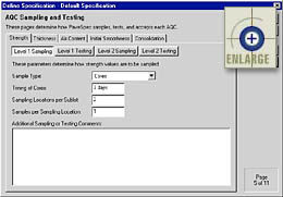 |
Figure 12. AQC Sampling and Testing dialogue box (Concrete Strength Sampling data entry screen). |
An example of the concrete strength testing data entry screen is shown in figure 13. The data inputs contained in this screen define the testing procedures to be used to measure concrete strength within the developed PRS. The testing-related inputs are divided into two groups: Testing and Acceptance.
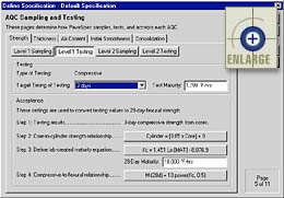 |
Figure 13.
AQC Sampling and Testing dialogue box (Concrete Strength Testing data entry screen). |
Within the testing group, the Type of Testing is provided as feedback. This testing type reflects the sample type chosen in the associated sampling data entry screen. The first input included in this testing group is the Target Timing of Testing. Use this input field to indicate the sample age at which testing is to be performed (e.g., if cylinders are to be tested at 7 days to obtain 7-day compressive strengths, this field should be set equal to 7 days). If the timing of testing is chosen to be less than 28 days, you must then enter an apporpriate Test Maturity value. This value should be equal to the equivalent laboratory maturity representing the chosen number of days selected in the Target Timing of Testing list box.
The
Acceptance group illustrates the steps required to estimate the
28-day flexural strength (required by the distress indicator models) based
on the chosen sample type and timing of testing. Each of these steps
will change based on the chosen sampling and testing procedures.
If a button is visible next to any step description, a specific relationship
needs to be defined by the user. For example, the ![]() button is visible next to step
2 in figure 13. This button indicates that the user must define
a cylinder vs. core relationship as part of the selected testing procedure.
Clicking on the
button is visible next to step
2 in figure 13. This button indicates that the user must define
a cylinder vs. core relationship as part of the selected testing procedure.
Clicking on the ![]() button brings up the Core-to-Cylinder Strength Relationship
dialogue box shown in figure 14.
button brings up the Core-to-Cylinder Strength Relationship
dialogue box shown in figure 14.
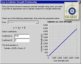 |
Figure 14.
Core-to-Cylinder Strength Relationship dialogue box. |
The dialogue shown in figure 14 is used to define the appropriate linear relationship between cylinder and core strength. The equation form is displayed directly beneath the Form box. Next, the coefficients defining the actual chosen relationship are defined in the supplied coefficient input boxes. The chosen equation coeffients are then shown in the actual developed equation displayed beneath the coefficient input boxes. Finally, the right side of the dialogue box shows a preview graph of the user-defined relationship. This preview graph is provided to help you visualize the defined relationship.
The button associated with concrete strength acceptance step 3 brings up a dialogue box (if required) that allows you to define the required Laboratory-Created Maturity Equation (strength versus maturity relationship). The Equation Definition dialogue box is nearly identical to the Core-to-Cylinder Strength Relationship dialogue box. The only difference is that the equation form is not limited to linear. Available equation forms include Linear, Second-Order Polynomial, Third-Order Polynomial, Exponential, Logarithmic, and Power. The final piece of information required under step 3 is the specified 28-day Maturity. This value is the equivalent maturity measured in the laboratory at 28 days.
Finally, the button associated with step 4 allows you to define an appropriate Compressive Strength-to-Flexural Strength relationship (if required). This pop-up dialogue box is also nearly identical to the Core-to-Cylinder Strength Relationship dialogue box (shown in figure 14). As with the pop-up dialogue box discussed for step 3, the only difference is that the equation form is not limited to linear. Available equation forms include Linear, Second-Order Polynomial, Third-Order Polynomial, Exponential, Logarithmic, and Power.
Selecting
the Thickness tab brings up a data entry screen used to define
the slab thickness sampling and testing plan. An example of this
data entry screen is shown in figure 15. If you chose to develop
a level 1 and level 2 specification at the same time, separate data entry
screens are provided for each specification level. You can toggle
between the level 1 and level 2 data entry screens using the ![]() and
and ![]() buttons. (Note: The level 1 and level
2 data entry screens are identical.) If you chose to only develop
a level 1 specification, only the
buttons. (Note: The level 1 and level
2 data entry screens are identical.) If you chose to only develop
a level 1 specification, only the ![]() button will be displayed.
button will be displayed.
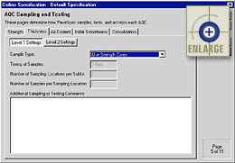 |
Figure 15.
AQC Sampling and Testing dialogue box (Slab Thickness data entry screen). |
The data inputs contained in this data entry screen define how slab thickness is to be sampled under the developed PRS. First, you must select a sample type from the Sample Type list box: Use Strength Cores, Independent Cores, Probe, or Ground-Penetrating Radar. If the sample type selected is Use Strength Cores, the remaining input boxes reflect the concrete strength sampling plan defined in the Strength tab.
Additional required slab thickness sampling plan inputs include the Timing of Samples, Number of Sampling Locations per Sublot, and Number of Samples per Sampling Location (replicates). Finally, you may enter any relevant notes in the Additional Sampling or Testing Comments text box (this field is optional).
Selecting
the Air Content tab allows you to define the entrained air content
sampling and testing plan. An example of this slab thickness sampling
and testing data entry screen is shown in figure 16. If you chose
to develop a level 1 and level 2 specification at the same time, separate
data entry screens are provided for each specification level. You
can toggle between the level 1 and level 2 data entry screens using the ![]() and
and ![]() buttons. (Note:
The level 1 and level 2 data entry screens are identical.) If you
chose to only develop a level 1 specification, only the
buttons. (Note:
The level 1 and level 2 data entry screens are identical.) If you
chose to only develop a level 1 specification, only the ![]() button will be displayed.
button will be displayed.
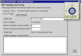 |
Figure 16. AQC Sampling and Testing dialogue box (Air Content data entry screen). |
The data inputs on this screen define how entrained air content is to be sampled under the developed PRS. You must first select one of the following three sample types provided in the Sample Type list box: Cores, Air Pressure Meter, or Danish Air Void Analyzer. If Cores is selected as the sample type, you must then specify when the cores are to be extracted from the pavement. (Note: The Timing of Samples input box is automatically set equal to At construction if the sample type selected is Air Pressure Meter or Danish Air Void Analyzer.) Next, you must define values for the other required entrained air content sampling plan inputs, including the Number of Sampling Locations per Sublot and Number of Samples per Sampling Location (replicates). Finally, you may enter relevant notes in the Additional Sampling or Testing Comments text box (field is optional).
Selecting
the Initial Smoothness tab allows you to define the sampling and
testing plan associated with measuring initial smoothness. An example
of this data entry screen is shown in figure 17. If you chose to
develop a level 1 and level 2 specification at the same time, separate
data entry screens are provided for each specification level. You
can toggle between the level 1 and level 2 data entry screens using the ![]() and
and ![]() buttons. (Note: The level 1 and level 2 data entry screens
are identical.) If you chose to only develop a level 1 specification,
only the
buttons. (Note: The level 1 and level 2 data entry screens
are identical.) If you chose to only develop a level 1 specification,
only the ![]() button will be displayed.
button will be displayed.
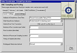 |
Figure 17. AQC Sampling and Testing dialogue box (Initial Smoothness data entry screen). |
The inputs required on this data entry screen define how initial smoothness is to be sampled under the developed PRS. First, you must select the indicator which you would like to use to express smoothness over time. Two indicators are available in the Indicator of Smoothness Over Time list box: Present Serviceability Rating (PSR) and International Roughness Index (IRI).
Second, you must select the appropriate Initial Smoothness Indicator that specifies how initial smoothness is to be measured. The following three Initial Smoothness Indicator types are availble:
Third, a button will appear (if required) that allows you to define a relationship between the chosen initial smoothness indicator and the initial smoothness over time indicator (PSR or IRI). This relationship is required to determine the initial PSR or IRI value in the prediction of smoothness over time. Based on the chosen settings for Indicator of Smoothness Over Time and Initial Smoothness Indicator, the appropriate equation type will be shown on the button. Clicking on the button will bring up the Define Initial to Over-Time Smoothness Indicator Translation Function dialogue box. This dialogue is nearly identical in layout and function to the Core-to-Cylinder Strength Relationship dialogue box shown in figure 14. Within this dialogue box, you can change the equation type or adjust the coefficients to define the appropriate smoothness-related relationship.
Other inputs included on this initial smoothness data entry screen include the Number of Pass Locations per Sublot and Number of Passes per Sampling Location (replicates). Additional text boxes are also included to allow you to enter comments related to the Pass Locations and the Timing of Samples (these two text fields are optional).
Percent Consolidation Around Dowels
Selecting
the Consolidation tab brings up a data entry screen used to define
the percent consolidation around dowels sampling and testing plan.
An example of this data entry screen is shown in figure 18. If you
chose to develop a level 1 and level 2 specification at the same time,
separate data entry screens are provided for each specification level.
You can toggle between the level 1 and level 2 data entry screens using
the ![]() and
and ![]() buttons. (Note:
The level 1 and level 2 data entry screens are identical.) If you
chose to only develop a level 1 specification, only the
buttons. (Note:
The level 1 and level 2 data entry screens are identical.) If you
chose to only develop a level 1 specification, only the ![]() button will be displayed.
button will be displayed.
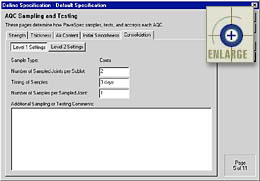 |
Figure 18.
AQC Sampling and Testing dialogue box (Percent Consolidation Around Dowels data entry screen). |
The data inputs contained in this data entry screen define how percent consolidation around dowels is to be sampled under the developed PRS. Under the current PRS approach, percent consolidation around dowels is measured by conducting relative density testing of core samples. Additional inputs required on this data entry screen include the Number of Sampled Joints per Sublot, Timing of Samples (timing of extracting cores), and the Number of Samples per Sampled Joint (replicates). You may also enter additional notes in the Additional Sampling or Testing Comments text box (this field is optional).
The as-designed target AQC target means and standard deviations are defined on page 6 of the Specification Wizard. If you chose to define a level 1 and level 2 specification at the same time, this dialogue box will contain two tabs titled Level 1 Settings and Level 2 Settings. If you only chose to develop a level 1 specification, only the Level 1 tab will be visible. The level 1 and level 2 data entry screens are identical, and an example is presented in figure 19.
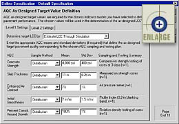 |
Figure
19. AQC As-Designed Target Value Definition dialogue box. |
First, you must decide on the method by which you would like to determine the as-designed target LCC. The following options are available:
The remainder of the data entry sheet contains input fields used to select the AQC as-designed target values. Only values for those AQC’s selected for inclusion in the PRS are required. The input fields for those AQC’s not included in the specification are grayed out, signifying that you cannot enter data.
If you choose to estimate the LCC through simulation, for each AQC included in the specification you must identify a Sample Method by which samples will be determined, a target AQC Mean value, and a target AQC standard deviation (Std Dev). You can choose from two different methods for determining samples within the simulation of the as-designed LCC: Include Variability or Means Only. If Include Variability is chosen, random as-designed samples are determined based on a normal distribution defined by the inputted AQC mean and standard deviation. If Means Only is chosen, sample values are assumed to be equal to the mean value that you entered. For this case, we assume that the variability of this AQC is not important. For example, let’s assume that concrete strength has been "specified" at 4,000 psi. Therefore, only one strength pay factor curve (the case for strength std dev = 0 psi) will be developed in the strength pay factor chart. All other pay factor curves will be simulated with the strength samples specified equal to 4,000 psi (with std dev = 0 psi). Similarly, if the Calculate LCC Using AQC Means Only option is chosen, all AQC pay factor charts will only contain one curve each (the case with std dev = 0).
As mentioned previously, PaveSpec uses English units as defaults. Values input in metric units are automatically converted to the corresponding English units. When entering an appropriate value in one of these input boxes, type the value followed by the appropriate units abbreviation (e.g., "254 mm"). Acceptable unit abbreviations for each AQC are as follows:
(Note: Within any numerical input box, you may toggle between default English and metric units using the " ` " key.)
Finally, the Sampling and Testing Summary area of the dialogue box provides feedback regarding the specific sampling and testing procedures defined on page 5 of the Specification Wizard. This information is important because the AQC target values typically differ for different sampling and testing procedures.
The life-cycle cost-related variables used in defining a specification are grouped into two types of module documents—Maintenance and Rehabilitation Plan and Unit Costs modules. Again, this organization not only simplifies the logic of the process, but it also allows you to save and reuse these groups of variables, which, in turn, simplifies the data entry itself. An example of the Life-Cycle Cost-Related Modules dialogue box is presented in figure 20.
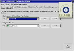 |
Figure 20. Life-Cycle Cost-Related Modules dialogue box. |
You
can access existing modules by clicking on the appropriate drop-down arrow
and highlighting the module you wish to use. To make changes to
a displayed module, click the ![]() button associated with that module type.
To create a new module, click on the
button associated with that module type.
To create a new module, click on the ![]() button. Whether
you decide to edit an existing module or create a new one, the data entry
screens will be the same (only the displayed input values will be different).
The data entry procedures for each module type will be discussed separately.
button. Whether
you decide to edit an existing module or create a new one, the data entry
screens will be the same (only the displayed input values will be different).
The data entry procedures for each module type will be discussed separately.
Maintenance and Rehabilitation Plan Module
An example of the dialogue box used to define a Maintenance and Rehabilitation Plan module is presented in figure 21. The Maintenance and Rehabilitation Plan dialogue includes a Name input box and four tabs titled Maintenance, Local Rehab, Global Rehab, and Description. By default, the Maintenance tab is displayed when you first enter into the Maintenance and Rehabilitation Plan dialogue box.
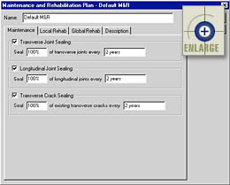 |
Figure 21. Maintenance and Rehabilitation Plan Module dialogue box. |
You can change the name of the Maintenance and Rehabilitation Plan module by entering a new name in the Name input box. The name you enter will show up as the specification document name in the Modules tab of the Database Control dialogue box.
Maintenance Tab
The Maintenance tab allows you to define the type, amount, and timing of routine maintenance activities used in the computation of LCC’s. Three different types of maintenance activities may be considered: transverse joint sealing, longitudinal joint sealing, and transverse crack sealing. To select one or more of these maintenance activities for inclusion in the M&R plan, click on the activity’s name or the corresponding check box.
The details of the routine maintenance plan are determined by defining: (1) how often the sealing crew will go to the field and (2) what percentage of joints or cracks will be sealed each time they go to the field. For example, if the agency typically seals 100 percent of transverse joints every 3 years on a repetitive schedule, the transverse joint sealing sentence should read "Seal 100% of transverse joints every 3 years." You should define each of these descriptive sentences carefully to match the routine maintenance methods actually used by your agency.
Local Rehab Tab
The Local Rehab tab (displayed in figure 22) allows you to define the localized rehabilitation plan in terms of a step-by-step prioritized procedure. Specifically, you can:
The complete list of localized rehabilitation steps is organized into a prioritized list in the main scroll box of this data entry screen.
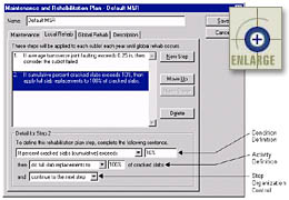 |
Figure 22. Local Rehab tab in the Maintenance and Rehabilitation Plan dialogue box. |
To create
a new step in the prioritized list, first select the step in the list
that you would like the new step to follow. Next, click on the ![]() button. If a step is accidentally inserted
in the wrong place, or if you wish to change the order of the steps at
any time, use the
button. If a step is accidentally inserted
in the wrong place, or if you wish to change the order of the steps at
any time, use the ![]() and
and ![]() buttons. To delete a step from the
list, highlight it and click on the
buttons. To delete a step from the
list, highlight it and click on the ![]() button.
button.
Condition Definition of a Localized Rehabilitation Step
The details making up each step in the prioritized list are defined using the input fields grouped at the bottom of the data entry screen. When an existing step is selected, the input settings making up the step description are defined by making changes in these input fields. Each step description is developed in the form of an If…then statement (i.e., if a certain pavement condition is present, then do activity X).
The first of the three lines of inputs (defined as the Condition Definition line, as shown in figure 22) is used to define a specific pavement condition. The first list box on the condition definition line allows you to select a pavement performance-related condition to which an action is to be applied. The list is mostly made up of predetermined "If" statements; however, you can also select to apply rehabilitation activities every year by selecting Always from the list, or at constant intervals (e.g., every 2 years) by selecting Every from this list. The different mechanisms available for determining when localized rehabilitation is applied are described below.
Applied at regular time intervals—If the agency is confident that it will apply a certain type of localized rehabilitation activity at regular time intervals over the life of a pavement, then select Every from the condition list. The second box in the condition definition line then becomes the input box for the specific time interval. For example, the condition definition line could read Every 3 years.
Based on individual sublot performance conditions—Using the PRS approach, the performance of each sublot is expressed in terms of predicted distress indicators. As stated in chapter 4 of volume I, it is recommended that the timing of the first global rehabilitation for a lot be based on the percentage of sublots determined to be failed (PSF). One method for determining if a particular sublot is failed is by comparing the predicted distress indicator levels to user-defined trigger values. The condition definition list box contains the following seven sublot pavement performance conditions to which defined trigger values may be applied:
- If percent cracked slabs (cumulative) exceeds…. This condition triggers on the cumulative percentage of cracked slabs (both fixed and unfixed).
- If percent cracked slabs (unfixed) exceeds…. This condition triggers on only the unfixed percentage of cracked slabs (i.e., cumulative percentage of cracked slabs minus the cumulative amount already fixed).
- If average transverse joint faulting exceeds….
- If percent spalled joints (cumulative) exceeds…. This condition triggers on the cumulative percentage of spalled joints (both fixed and unfixed).
- If percent spalled joints (unfixed) exceeds…. Triggers on only the unfixed percentage of spalled joints (i.e., cumulative percentage of spalled joints minus the cumulative amount already fixed).
- If PSR is less than….
- If IRI is greater than….
If any of these seven items is selected, the second condition definition input box becomes the input box for the corresponding trigger value. The appropriate units for the corresponding trigger values are the following:
- Percent cracked slabs—Default unit for this trigger value is "%".
- Average transverse joint faulting—Acceptable metric abbreviations include "cm" and the default units of "mm", with the default English values in terms of "in".
- Percent spalled joints—Default unit for this trigger value is "%".
- PSR—This indicator is expressed as a number between 0 and 5; it is dimensionless.
- IRI—Metric values are expressed in terms of "mm/km", while English values are in terms of "in/mi".
Based on the cumulative amount of applied localized rehabilitation for an individual sublot—An individual sublot may also be considered failed if certain amounts of repairs (localized rehabilitation) have been applied (e.g., the sublot is considered failed if 35 percent of the total slabs have been replaced). The condition definition list box contains the following four sublot cumulative localized rehabilitation conditions to which defined trigger values may be applied:
- If repaired joints per mile exceeds….
- If percent of repaired joints exceeds….
- If repaired slabs per mile exceeds….
- If percent of repaired slabs exceeds….
If any of these four items is selected, the second condition definition input box becomes the input box for the corresponding trigger value. The appropriate units for the corresponding trigger values are the following:
- Repaired joints per mile—This indicator is expressed as a number with no dimensions.
- Percent of repaired joints—Default unit for this trigger value is "%".
- Repaired slabs per mile—This indicator is expressed as a number with no dimensions.
- Percent of repaired slabs—Default unit for this trigger value is "%".
Based on the lot average of sublot performance conditions—If you do not want to use the percentage of sublots failed approach for determining the timing of the first global rehabilitation application, you can choose to base this event on the average of the yearly predicted sublot distresses. In other words, at each year of the analysis life, the individual sublot distresses are computed and then averaged for the entire lot. These lot averages of yearly sublot distresses are then compared to user-defined trigger values to determine the timing of the first global rehabilitation application. The condition definition drop-down box contains the following five lot average conditions to which defined trigger values may be applied:
- If lot average percent cracked slabs exceeds….
- If lot average transverse joint faulting exceeds….
- If lot average percent spalled joints exceeds….
- If lot average PSR is less than….
- If lot average IRI is greater than….
If any of these five items is selected, the second condition definition input box becomes the input box for the corresponding trigger value. The appropriate units for the corresponding trigger values are the following:
- Lot average percent cracked slabs—Default unit for this trigger value is "%".
- Lot average transverse joint faulting—Acceptable metric abbreviations include "cm" and the default units of "mm", whereas English values are expressed in terms of "in".
- Lot average percent spalled joints—Default unit for this trigger value is "%".
- Lot average PSR—This indicator is expressed as a number between 0 and 5; it is dimensionless.
- Lot average IRI—Metric values are expressed in terms of "mm/km", while English values are in terms of "in/mi".
The last input in the condition definition drop-down box is If percent sublots failed exceeds…. This allows you to use the percent sublots failed (PSF) condition that will trigger the first application of a global rehabilitation. If this item is selected, the second condition definition input box becomes the input box for the corresponding trigger value. The PSF trigger value is expressed in units of "%".
Activity Definition of a Localized Rehabilitation Step
Once a specific condition is defined, you must determine what type of activity to apply in response to it. The second line of input fields in the Localized Rehab data entry tab (referred to as the Activity Definition line, as shown in figure 22) is used to define this responsive activity. The available activity items are described below.
Do nothing—You have the option to select Do no rehab for this step from the activity list. If this item is selected, the remaining input boxes making up the Activity Definition line disappear.
Apply localized rehabilitation in response to individual sublot performance conditions—If you have selected a condition item that defines a trigger on an individual sublot performance condition (e.g., If percent cracked slabs exceeds 10%), then the following localized rehabilitation-responsive activities are available:
- Do partial slab replacements to….
- Do full slab replacements to….
- Do full-depth repairs to….
- Do partial-depth repairs to….
If any of these four items is selected in the activity input list box, the second input box will allow you to input a percentage of the cracked slabs or spalled joints that will be replaced during the year. Those cracked slabs or spalled joints that are not fixed during a particular year are carried over to the next year.
Note: The localized rehabilitation activities are limited to repairing cracked slabs (transverse slab cracking) or spalled joints (transverse joint spalling). The effects of transverse joint faulting and pavement smoothness (PSR or IRI) are addressed with global rehabilitation.
Designate the sublot as failed—If the PSF method is being used to determine the timing of the first global rehabilitation application, you need a method to designate the sublot as failed. Therefore, in response to a defined set of individual sublot performance conditions, or cumulative applied localized rehabilitation, you can choose the consider the sublot failed activity item.
Apply a global rehabilitation scenario—You may choose to apply a global rehabilitation in response to any of the available condition types. The activity list contains three predefined global rehabilitation scenarios (these will be discussed under the explanation of the Global Rehab tab). These correspond to the following three choices contained in the activity input list:
- Begin global rehab scenario 1.
- Begin global rehab scenario 2.
- Begin global rehab scenario 3.
Step Organization Control
The third line of input fields in the Localized Rehab data entry tab (referred to as the Step Organization Control input, as shown in figure 22) provides some additional control for determining the behavior of the prioritized list. This drop-down box contains the following three inputs:
These determine what action is to be taken after the defined activity of a step is applied. The default value for this input list box is Continue to the next step; however, the other two options become very useful when organizing a complicated prioritized list.
Global Rehab Tab
The Global Rehab tab allows you to define up to three different global rehabilitation scenarios. Each scenario includes the localized rehabilitation to be completed before the first global rehabilitation application, as well as details of how global rehabilitations are to be applied over the analysis period. An example of the Global Rehab tab is displayed in figure 23.
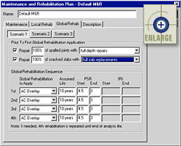 |
Figure 23. Global Rehab tab in the Maintenance and Rehabilitation Plan dialogue box. |
The Global Rehab tab contains buttons that allow you to define up to three different global rehabilitation scenarios. (Note: The input fields are identical within each of the three scenario data entry screens.)
On the Global Rehab screen, the first area (titled Prior to First Global Rehabilitation Application) allows you to define the types and amount of localized rehabilitation to be completed prior to applying the first global rehabilitation. The localized rehabilitation is limited to repairing cracked slabs (due to transverse slab cracking) or repairing transverse joints (due to transverse joint spalling). You may first select which of these localized rehabilitation types to apply (if any) by clicking on the corresponding check box. If a localized rehabilitation type is selected for inclusion, you must enter the percentage (between 0 and 100 percent) of cracked slabs or spalled joints you wish to repair, then select the method to be used to repair them.
The second area on this screen (titled Global Rehabilitation Sequence) is used to define the details of the global rehabilitation schedule making up the scenario. The scenario allows you to define different global rehabilitations up until the fourth application. For example, you could choose to apply diamond grinding for the first two scheduled global rehabilitations and asphalt overlays for all subsequent applications. You must also input an assumed life for each chosen global rehabilitation (i.e., number of years until next global rehabilitation is applied), as well as an assumed smoothness value in terms of chosen smoothness over time indicator (PSR or IRI) at the start and end of the global rehabilitation’s life. The smoothness during the defined rehabilitation life is assumed to decrease linearly from the chosen starting smoothness value to the chosen ending smoothness value.
Description Tab
The Description tab contains a text box in which you may enter any detailed text describing the defined Maintenance and Rehabilitation Plan module. Information entered in this tab is not used in the simulation process, so it is completely optional. An example of the Description tab is shown in figure 24.
 |
Figure 24. Description tab in the Maintenance and Rehabilitation Plan dialogue box. |
Saving or Exiting the Maintenance and Rehabilitation Plan Module Dialogue Box
Once
you are finished defining a Maintenance and Rehabilitation Plan
module, click on the ![]() button to save your named module. If you
would like to exit the Maintenance and Rehabilitation Plan dialogue
box without saving your changes, click on the
button to save your named module. If you
would like to exit the Maintenance and Rehabilitation Plan dialogue
box without saving your changes, click on the ![]() button. Clicking
either button will return you to the Life-Cycle Cost-Related Modules
dialogue box.
button. Clicking
either button will return you to the Life-Cycle Cost-Related Modules
dialogue box.
An example of the dialogue box used to define a Unit Costs module is presented in figure 25. The Unit Costs dialogue box includes a Name input box and three tabs titled Maintenance, Rehabilitation, and Other. By default, the Maintenance tab is displayed when you first enter the Define Unit Costs dialogue.
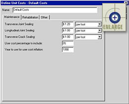 |
Figure 25. Define Unit Costs dialogue box. |
You may change the name of the Unit Costs module by entering a new name in the Name input box. The name you enter will show up as the specification document name in the Modules tab of the Database Control dialogue box.
Maintenance Tab
The maintenance-related unit costs are defined in the Maintenance tab of the Define Unit Costs module dialogue box (shown in figure 24). For each listed maintenance activity, you must input an appropriate unit cost in dollars and select the appropriate unit from the corresponding list box.
Rehabilitation Tab
The localized and global rehabilitation-related unit costs are defined in the Rehabilitation tab. An example of the Rehabilitation tab is shown in figure 26. For each listed rehabilitation activity, you must input an appropriate unit cost in dollars and select the appropriate unit from the corresponding list box.
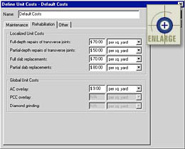 |
Figure 26.
Rehabilitation tab in the Define Unit Costs dialogue box. |
Other Tab
The Other tab contains miscellaneous unit cost-related items required to compute LCC’s. For example, the interest and inflation rates required for determining present-worth LCC’s are included in this tab (Discount Rate = Interest Rate – Inflation Rate). Other input boxes include the assumed width of a full-depth or partial-depth joint repair (required if the joint repair unit cost is expressed in terms of dollars per area) and the assumed width of a partial slab replacement.
A text box is also included in which you may enter text describing the defined Unit Cost module. This field is optional. An example of the Other tab in the Define Unit Costs dialogue box is presented in figure 27.
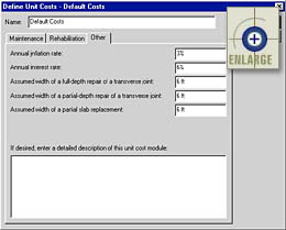 |
Figure 27.
Other tab in the Define Unit Costs dialogue box. |
Saving or Exiting the Define Unit Costs Module Dialogue Box
Once
you are finished making changes or defining a Unit Cost module,
click on the ![]() button to save your named
module. If you would like to exit the Unit Cost dialogue
box without saving your changes, click on the
button to save your named
module. If you would like to exit the Unit Cost dialogue
box without saving your changes, click on the ![]() button. Clicking either button
will return you to the Life-Cycle Cost-Related Modules dialogue
box.
button. Clicking either button
will return you to the Life-Cycle Cost-Related Modules dialogue
box.
Details regarding the simulation process are defined on page 8 of the Specification Wizard. The tab displayed when you first enter this page, titled Generic Settings, contains all of the simulation parameters that do not change between a level 1 and level 2 specification. The additional tabs depend on the AQC’s you selected to include in the specification. Clicking on the appropriate AQC tab will bring up a data entry screen used to define the level 1 pay factor curves for that AQC. An example of the Simulation Control dialogue box is presented in figure 28.
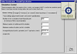 |
Figure 28.
Simulation Control dialogue box. |
The Generic Settings tab is made up of five different inputs that define the simulation procedures used to develop level 1 and level 2 preconstruction output. First, you must define the number of lots used to simulate each factorial point (a value of 500 is recommended). If this value is set at 500, it means that the level 2 as-designed LCC will be computed as the average of 500 simulated lot LCC’s. For the level 1 pay factor curves, each simulated point used to define each curve will also be based on the average of 500 simulated lot LCC’s.
The second and third inputs in the Generic Settings tab define the minimum and maximum number of sublots per lot to be considered in the simulations. These inputs are required because an agency never knows ahead of time (i.e., before going out into the field) how many sublots will make up the next lot. Since the number of sublots per lot affects the computed pay factors, the program allows you to simulate the same specification for different numbers of expected sublots per lot. The minimum and maximum sublots selected in these inputs defines the range over which preconstruction output will be simulated. For example, if you select to simulate 1 to 4 sublots per lot, different level 1 pay factor curves will be developed for the cases of 1, 2, 3, and 4 sublots. For the level 2 specification, four different as-designed LCC’s (representing 1, 2, 3, and 4 sublots) will be simulated.
The fourth input on this tab is the assumed contractor bid price used to compute the level 1 pay factors. It is recommended that this assumed price be an average contractor bid price computed using historical agency bid price data. This input may be entered in metric units of "$/m2" or English units of "$/yd2".
Finally, the last input in the Generic Settings tab defines the analysis life used for computing LCC’s. This is the period of time over which future M & R costs are to be considered in the LCC analysis.
The tabs for the included AQC’s are identical in layout and function. Each AQC-related tab is provided to define the level 1 pay factor curves (for the specific AQC) that make up the level 1 preconstruction output. An example of one of these tabs (Strength) is presented in figure 29.
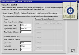 |
Figure 29. Example of an AQC-related tab within the Simulation Control dialogue box. |
Each AQC-related tab is used to define a factorial design of combinations of AQC mean and standard deviation. The simulated pay factors are used to develop level 1 pay factor curves. The AQC-related tab is divided into the following three areas:
The simulation of preconstruction output begins on page 9 of the Specification Wizard. The Building Document and Preconstruction Output dialogue box is provided as a status window for this simulation process. An example of this dialogue box is presented in figure 30.
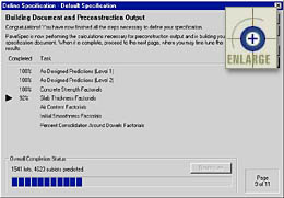 |
Figure 30.
Building Document and Preconstruction Output dialogue box. |
The dialogue box is divided into two parts. The first part contains a list of the different tasks being performed, including initializing (building) the specification output document, conducting the as-designed simulations, conducting the simulations defined in the AQC level 1 factorials, and summarizing the simulated data. The percentage completed is displayed beside each task description.
An Overall Completion Status bar is also included at the bottom of the dialogue box. This status bar illustrates the in-progress status of the number of lots and sublots being predicted (simulated). When complete, the visual status bar will be replaced with a message that states, The document is up-to-date with your specification settings. If changes are made in any previous step of the Specification Wizard after the simulation is complete, the specification document will be resimulated when you get to this page.
After the specification has been simulated, the Level 1 Preconstruction Output Control dialogue box allows you to specify the level 1 regression equations fit through the simulated pay factor data. An example of this dialogue box is presented in figure 31.
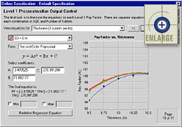 |
Figure 31. Level 1 Preconstruction Output Control dialogue box. |
The first list
box, View equations for, contains a list of all the simulated
pay factor charts. Each chart represents the simulated data for
the combination of one AQC and one number of sublots per lot.
For example, if you selected all five AQC’s for inclusion in the
specification, and you chose to simulate level 1 preconstruction output
for four different numbers of sublots per lot, then this list box will
contain 5 * 4 = 20 level 1 pay factor charts. You may view any
pay factor chart by selecting it from the View equations for
list box or by using the ![]() and
and ![]() buttons to scroll through the list.
buttons to scroll through the list.
Each pay factor chart contains simulated data making up the pay factor curves. Each pay factor curve is specific to one standard deviation. The area on the left side of the Level 1 Preconstruction Output Control dialogue box contains a number of different input fields used to specify the pay factor curves and corresponding equations. You can select a particular pay factor curve within the selected pay factor chart using the drop-down box just below the View equations for box. This box lists all the available pay factor curves by AQC standard deviation. This list is also color-coded to match the curves in the displayed pay factor chart.
After you select a specific pay factor curve, you may use the remaining input fields to define the regression equation representing this curve. The first step is to select the regression equation form you would like to use. The program provides five different equation forms: linear, second-order polynomial, third-order polynomial, exponential, and logarithmic. An example of the chosen equation form is displayed below the Form box.
By
default, when you first select a different equation form, the displayed
coefficients are those automatically determined by the program’s
regression analysis tool. The final equation (including coefficients)
will be displayed at the bottom of the dialogue box. You may also
choose to change the equation coefficients. If you wish to reset
the coefficients to those determined automatically by PaveSpec, simply
click on the ![]() button.
button.
It is recommended that you view each pay factor curve independently to make sure that you are content with the defined curve and corresponding equation. The level 1 individual AQC pay factor equations defined in this dialogue box will be used in the field to compute level 1 individual AQC contractor pay factors.
To compute an overall level 1 lot pay factor, a level 1 composite pay factor equation needs to be defined as a function of the individual AQC level 1 pay factors. This dialogue box allows you to define the actual composite pay factor equation to be used in the computation of contractor pay factors. An example of this composite pay factor-related dialogue box is presented in figure 32.
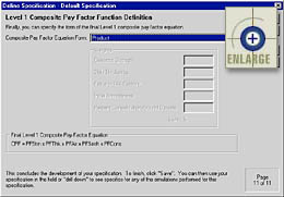 |
Figure 32. Level 1 Composite Pay Factor Equation Definition dialogue box. |
First, you must choose the composite pay factor equation form from the provided list box. Five different equation forms are provided for use within PaveSpec: Simple Average, Weighted Average, Product, Minimum, and Maximum. If Weighted Average is chosen as the equation form, the individual weighting factors are entered in the provided input boxes. The final defined Level 1 composite pay factor equation, used in the computation of actual contractor pay factors, is then displayed toward the bottom of this dialogue box.