U.S. Department of Transportation
Federal Highway Administration
1200 New Jersey Avenue, SE
Washington, DC 20590
202-366-4000
Federal Highway Administration Research and Technology
Coordinating, Developing, and Delivering Highway Transportation Innovations
 |
| This report is an archived publication and may contain dated technical, contact, and link information |
|
Publication Number: FHWA-HRT-07-021
Date: April 2007 |
|||||||||||||||||||||||||||||||||||||||||||||||||||||||||||||||||||||||||||||||||||||||||||||||||||||||||||||||||||||||||||||||||||||||||||||||||||||||||||||||||||||||||||||||||||||||||||||||||||||||||||||||||||||||||||||||||||||||||||||||||||||||||||||||||||||||||||||||||||||||||||||||||||||||||||||||||||||||||||||||||||||||||||||||||||||||||||||||||||||||||||||||||||||||||||||||||||||||||||||||||||||||||||||||||||||||||||||||||||||||||||||||||||||||||||||||||||||||||||||||||||||||||||||||||||||||||||||||||||||||||||||||||||||||||||||||||||||||||||||||||||||||||||||||||||||||||||||||||||||||||||||||||||||||||||||||||||||||||||||||||||||||||||||||||||||||||||||||||||||||||||||||||||||||||||||||||||||||||||||||||||||||||||||||||||||||||||||||||||||||||||||||||||
Durability of Segmental Retaining Wall Blocks: Final ReportCHAPTER 4: LABORATORY EVALUATIONS4.1 OVERVIEWThis chapter summarizes a comprehensive laboratory evaluation focusing on the frost resistance (with and without salts) of SRW blocks. The chapter is based upon the research described in Chan (2006), Hance (2005), and Haisler (2004), as well as the other technical documents produced under this FHWA project (see section 1.4). Because of the extensive amount of laboratory work performed in this project, efforts have been made to synthesize the key research and to present only the most important and relevant results with an eye toward which ones can or should be implemented into accelerated test methods and specifications to ensure long-term durability of SRW blocks in aggressive, cold environments. Much of the research described in this chapter is related to ASTM C 1262 (2003), which was the most commonly used test method for assessing freeze-thaw durability of SRW blocks when this project was initiated. Because this method was being used and/or specified by a number of SHAs, including those States that reported durability problems associated with SRWs, the decision was made from the onset of this project to focus on refining and improving reliability and reproducibility of the test. To elaborate on this point, it should be noted that ASTM C 1262 (2003) test had received significant criticism from end users due to concerns over the repeatability of test results, even within one set of samples from the same lot of SRW blocks. There were also questions as to the actual relation between the test results and field exposure conditions and performance. Given the shortage of previous published research on this general topic (frost resistance of SRW blocks) and on this specific issue (test methods to predict field performance), fundamental research was initiated to improve the understanding of the distress mechanisms associated with SRW blocks and in properly testing potential SRW blocks for use in aggressive environments. Figure 27 shows the overall scope of research that was performed on the various aspects of ASTM C 1262 (2003), with the basic information on each of the areas of concentration. It is not feasible to discuss in detail all of these aspects of the research program; figure 27 provides the reader with the overall scope of the efforts launched under this project. It should also be noted that some of the research focusing on damage assessment methods was performed in a separate research project funded by National Concrete Masonry Association (NCMA), but this work was performed by essentially the same research team as the FHWA project, and the work was done parallel to the research described in this project report. Only a brief synopsis of these NCMA-funded efforts is presented herein.
The remainder of this chapter is organized as follows:
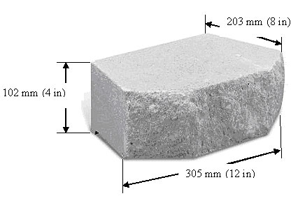
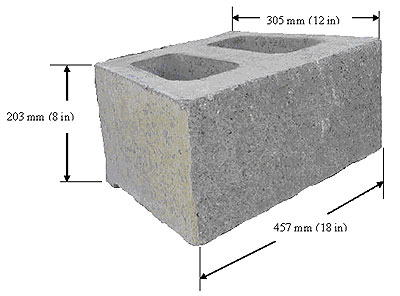
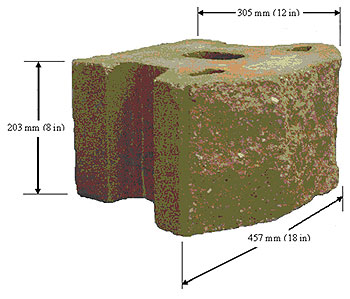
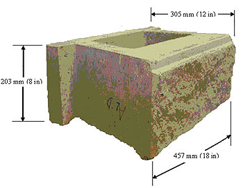
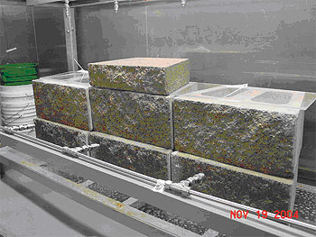
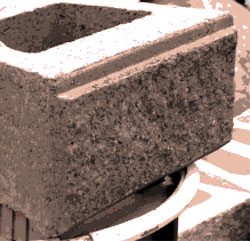
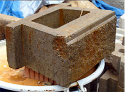
4.2 SAMPLING CONSIDERATIONS FOR SRW BLOCKSOne of the initial steps in the freeze-thaw testing of SRW units involves extracting test specimens from representative units. These steps are covered in sections 6 and 7 of the ASTM C 1262 (2003) standard. The specific manner in which a laboratory technician selects the units and extracts test specimens from them may influence the outcome of test results, as will be described in this section. Before proceeding further, a brief overview of the manufacturing process is provided. SRW units are manufactured in block plants typically by compacting (while simultaneously vibrating) concrete mixes into steel molds, followed by immediate removal of the molds. The shaped units are subsequently conveyed to curing chambers maintained at elevated temperatures and humidity where the units are kept for a certain time period (which may be variable) before being withdrawn. In one plant visited in early 2004, residence time of SRW units in the curing chamber was understood to last anywhere from 1 to 3 days, depending on production schedule. In many cases, units are cast as sets of conjoined pairs, which are then split in the middle to produce a natural-looking or "split face" fractured surface. Following splitting, the units are stacked on pallets and stored in a nonstandard manner. These steps are illustrated in figures 28 through 31. From this description and in reference to figure 32, the following locations on the units are identified for the solid and hollow units shown in the figure:
Also shown is the height, H, of the units for which 200 mm (8 inches) and 150 mm (6 inches) are common dimensions. For the rest of this report, the term unit will be used to refer to a whole block as produced in manufacturing plants, as shown in figures 32 and 33. Specimens or coupons are typically cut from the units for testing such as ASTM C 140 (2000) tests for compressive strength, absorption and density and ASTM C 1262 (2003) freeze-thaw tests. ASTM C 1262 (2003) uses the words specimens and coupons interchangeably, as does this report.
4.2.1 Current Sampling GuidelinesIn the procurement of test specimens from SRW units, there are two levels of sampling. The first is sampling of SRW units from lots (defined below) and the second is extraction of test specimens from individual units. This research project did not investigate the first level of sampling in detail; however, some general comments are provided. As for sampling units from lots, section 6 of ASTM C 1262 (2003) states the following: Clause 6.1: "Select whole units representative of the lot from which they are selected. The units shall be free from visible cracks or structural defects." Clause 6.2 "Select five units for freezing and thawing tests." Meanwhile, ASTM C 140 (2000) defines "lot" as follows (Clause 4.1.2): Any number of concrete masonry units of any configuration or dimension manufactured by the producer using the same materials, concrete mix design, manufacturing process, and curing method While this clause provides a generalized statement of what a "lot" encompasses, various details of this definition still remain unclear. The length of production time (1 year, 1 month, one project or one batch) during which "the same materials, concrete mix design, manufacturing process, and curing method" were used is not clear. The manner in which units are to be selected from the lot also remains vague. For example, are units to be randomly sampled as they come out of the production line, or are units to be sampled from pallets during storage at the block plant or at a jobsite? ASTM C 140 (2000) includes curing method as one characteristic of a lot, but it does not necessarily imply curing time or duration. Production plant logistics play a role in determining how long SRW units are kept in the curing chamber. This is critical because the overall quality of concrete varies with early-age curing; and whether units are cured for 1 day or 3 days plus curing conditions (temperature and relative humidity) impact the quality of the material. Furthermore, depending on ambient weather conditions, the storage condition of the SRW units is critical, as illustrated by the picture in figure 34. Units sampled from within a pallet that is shrink-wrapped may be of different quality than ones from unprotected pallets, as shown in this figure. When extracting test specimens from SRW units, ASTM C 1262 (2003) requires "saw-cutting solid coupons (test specimens) from full sized units" (Clause 7.1), and for units with exposed nonplanar surface which could be split, fluted or ribbed, the coupon should be cut "from another flat molded surface" (Clause 7.1.1). Aside from these statements, there is no further indication of where or how these specimens should be sampled within parent units. As will be discussed in the next sections, material properties within SRW units vary systematically with location, and thus a simple random scheme for specimen extraction (whereby specimens are extracted from random locations over a unit) may not work. An alternate method known as stratified random sampling is shown to reduce variability. The challenge in sampling equally applies to ASTM C 1262 (2003) specimens extracted for freeze-thaw testing or ASTM C 140 (2000) specimens extracted for material property determination.
Two different philosophies with respect to sampling are possible depending on the intended purpose of the tests. These are:
In the first case, it may be desired to sample whole units and extract specimens from these units in such manner that variability between test specimens is reduced. Ways in which this can be achieved are described in this chapter. For site acceptance of units, however, it is more sensible to sample units that are most vulnerable (i.e., of lowest quality among the population of units) and to extract specimens from the most vulnerable locations within the unit. The following sections describe how quality varies over a unit and how knowledge of this variation helps with the decision on choosing samples from units. 4.2.2 Spatial Variability of Material Properties4.2.2.1 Within-Manufacturer VariabilityStudies were conducted to investigate spatial variation in selected material properties in SRW units obtained from a single block manufacturer (Chan et al., 2005a and b). These units are depicted in figures 35 through 38. Figures 35 and 36 were referred to as large wall unit, and figures 37 and 38 were referred to as small wall unit. Specimens from each of these types of SRW units were extracted in the manner shown in the figures and tested for flexural strength to ASTM C 78 (ASTM 2002), flexural elastic modulus, 24-hour absorption to ASTM C 140 (2000), and boiled absorption to ASTM C 642 (ASTM 2002). An example of the spatial distribution in the 24-hour water absorption observed in these units is shown in figures 35 through 38. The values shown in this figure are average values across each of the rows of specimens shown (i.e., four specimens per row in the front face of large wall units, two to three specimens per row in the back face of large wall units, and two to three specimens per row in the small wall units). Three units were tested for each type of wall unit (large or small), and each of these units showed similar patterns in the measured properties, as follows:
Flexural strength and flexural elastic modulus, followed the same trend, although inverse of absorption (i.e., locations exhibiting lower absorptions displayed higher flexural strength and flexural elastic modulus, while locations exhibiting higher absorptions displayed lower flexural strength and flexural elastic modulus). These patterns altogether suggested that the material in the middle layer on the front face was likely of lowest quality (highest absorption and lowest flexural strengths and moduli) in the unit, while material in the back face was likely of higher quality (Chan et al., 2005a). A general linear model (GLM) analysis (Ott 1993) was also performed on the absorption data to verify the statistical significance of trends at the 95 percent confidence level (Chan et al., 2005b). This model confirmed a parabolic distribution of absorption along the casting direction (along the y-axis shown in the figure with maximum absorption in the middle layer), and a linear distribution of absorption in a direction from front to back face (with maximum absorption at the front face and minimum at the back face). These distributions are depicted in figures 35 through 38. No statistically significant distributions were detected along the x-axis. Systematic spatial variations of properties in the SRW units tested suggest that the specific method of sampling alone can lead to disparate test results. For instance, on the front face of the large wall unit shown in figures 35 and 36, water absorption values of specimens in the middle layer were 24 percent higher than those in the bottom layer; while on the back face, water absorption values of specimens in the middle layer were up to 60 percent higher than those in the bottom layer. This indicates that extraction of test specimens from random locations without consideration of the forms of distribution augments test variability. To reduce apparent variability due to the spatial distributions of properties, an alternate sampling scheme known as stratified random sampling (as opposed to simple random sampling) can be employed (Chan et al., 2005b). The difference between these two methods is shown in figure 39 for sampling from 12 possible locations on the face of an SRW unit. In simple random sampling, replicate specimens in a test set are randomly extracted from the various locations, tested for a particular material property and their results averaged. On the other hand, in stratified random sampling, specimen sampling is carried out in a more systematic manner reflecting the expected distribution of properties (Lohr, 1999). For the types of distribution observed here, an equal number of specimens is extracted from each of the rows or strata (three shown in Figure 39) to form the test set. Other size test sets consisting two or five specimens can also be selected under stratified random sampling, but the computation of average value of the measured property for the test set needs to be adjusted accordingly. Details on this calculation are covered in Chan et al. (2005b). This technique yields results that are more representative of the overall unit and is shown to reduce the apparent variability in test results. For the population of front face specimens, it is demonstrated that test variability (as measured by coefficients of variation) is reduced by approximately one-third when using stratified random sampling as opposed to Simple Random.
It should be emphasized that stratified random sampling yields results that are more representative of the entire SRW unit and with lower variability. This approach may not be applicable in cases where the quality of the entire SRW unit (i.e., at every location on the unit) needs to comply with minimum quality standards, such as ASTM C 1372 (2003) for compressive strength, absorption, and density. In these cases, sampling from the middle layers is preferred because material in this layer is typically of lowest quality in a given face of the unit. Compliance with specifications of this middle layer thus increases the likelihood that the unit overall is satisfactory. 4.2.2.2 Between-Manufacturer VariabilityThe studies described in the previous section focused on systematic spatial variations in material properties in SRW units from a single, residential-grade manufacturer. Further investigations were conducted to determine whether similar trends also existed in SRW units from other manufacturers producing commercial grade units. SRW units from four major block manufacturers (identified as Manufacturers A, B, C and D) were also evaluated for systematic spatial distributions of properties. Complete details and results of this investigation on spatial variability are provided in Chan et al. (2006c). A brief discussion is presented here. Each of the four participating manufacturers were asked to provide two grades of SRW units:
DOT units generally possessed denser internal structure with higher paste volume and lower compaction void volume, and freeze-thaw durability compliant with ASTM C 1372 (2003) or State specifications. On the other hand, most non-DOT units had a leaner internal structure and contained larger volume of compaction voids. The various types of SRW units were then labeled as follows: A-D (for Manufacturer A, DOT unit), A-N (for Manufacturer A, non-DOT unit), B-D, B-N, C-D, C-N, D-D and D-N. Mixture designs, production methods or curing, and storage details of these units were not available. Similar block samples from each manufacturer were also tested using ASTM C 1262 (2003) (in water and saline), and these results will be discussed later in this chapter. For these units, only the front (split) faces were evaluated, and specimens were extracted at approximately 25 to 50 mm (0.98 inch to 1.96 inch) from the split surface, as shown in figure 40a. As in the previous studies, three layers along the casting direction were also considered. Figure 40b shows the features on the side faces of the SRW units that were used as position references to identify the exact locations of specimen extraction. These side faces were referred to as either lipped/grooved (containing intentional indentations, ledges, or both), and flush side (consisting of a smooth surface with no features). Material properties evaluated in these SRW units included the following:
Figure 40. Drawing and photos. Sampling of test specimens from SRW units from different manufacturers. Examples of the spatial distribution exhibited by some of these properties are shown in figure 41 for ASTM C 642 (2002) boiled absorption, figure 42 for volumetric paste content, and figure 43 for volumetric compaction void content. The values shown in these figures represent the average absorption value of specimens in each of the layers shown (typically three to four specimens per layer). As with the SRW units described in section 4.2.2.1, variations in the measured values of these properties could arise depending on where samples were extracted from. For example, for unit C-D, samples taken from the middle layer showed 23 percent higher boiled absorption, 3 percent lower paste contents, and 63 percent higher compaction void contents compared to samples extracted near the lipped/grooved side. Also, as with the SRW units described in the previous section, the middle layer showed highest absorption of all sampled locations on this particular face. A perhaps more significant observation was the consistency in the locations where maximum or minimum values occurred for various properties. As demonstrated in figures 41, 42, and 43, boiled absorption was generally highest in the middle layer of the units, which is also where paste volume was generally lowest and compaction void volume highest. Oven-dried density was also lowest in this layer (Chan et al., 2006c). Although these observed relationships in the properties were as expected, the consistency in the locations where maximum values occurred indicated that the above distributions were not random, but systematic in nature. These trends occurred similarly for all manufacturers and SRW unit grades evaluated, suggesting that these distributions in properties were likely tied to the manufacture of SRW units. As before, stratified random sampling methods would be more applicable for these units compared to simple random sampling. From the preceding sections, it is evident that spatial distributions of material properties in SRW units were systematic in nature, and their statistical significance was demonstrated for units from a single manufacturer. While it is suspected that these distributions are related to manufacturing processes such as compaction and curing (Chan et al. 2005a), the existence of these patterns lead to several consequences. First, from a mix qualification standpoint, there may be units of lower quality compared to the ones tested here where sampling location could make the difference between compliance and noncompliance. For example, if the overall average water absorption of a given unit was hypothetically right on the specification limit for this property, specimens extracted from the middle layers would be found noncompliant, while specimens extracted from the outer layers would be found compliant. Second, due to spatial distributions of properties, the interpretation of material variability, operator variability or test method variability will be affected by sampling location. For the units described here, a laboratory technician who consistently chose to sample from the middle layers would obtain different results from a technician who consistently chose to sample from the outer (top and bottom) layers. Finally, the observed spatial patterns in various material properties such as absorption, flexural strength, compaction void content, and density imply that other properties such as permeability and freeze-thaw durability will vary from location to location within an SRW unit.
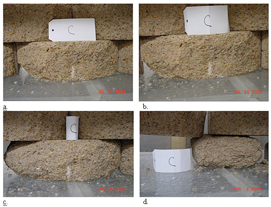
4.2.3 Split Face DelaminationOne advantage of SRW systems rests on the aesthetic appearance offered by the front split surface of the SRW units. A closer look at this surface, however, often reveals thin delaminations or cracked sections of varying sizes, as shown in figures 44 and 45. These cracked sections are referred to here as split face delaminations. Chan et al. (2006a) discuss the possible origins of these delaminations, as well as the significance these may have on the evaluation of SRW unit condition both in the field and in the laboratory. As for their cause, it is suspected that split face delaminations are created in the manufacturing of SRW units during the splitting process. As shown earlier in figures 28 through 31, splitting of conjoined units is accomplished by pressing steel knife edges at the preformed notch location to be split and forcing the units to crack at this plane. Cracks emanating from the edges of the units may merge as they approach one another, as shown in figure 46a, leaving behind fractured sections in the split plane. This interaction between approaching cracks was simulated using a linear elastic fracture mechanics model (using the software FRANC2D, Cornell University, 2002) shown in figure 46b. The fractured sections left behind after crack merging are believed to constitute split face delaminations. Further support to this suggested mechanism was obtained from visual observations at a local manufacturing plant. Figure 46c shows a view of the split face of one unit immediately after being split, where a detached split face delamination is seen.
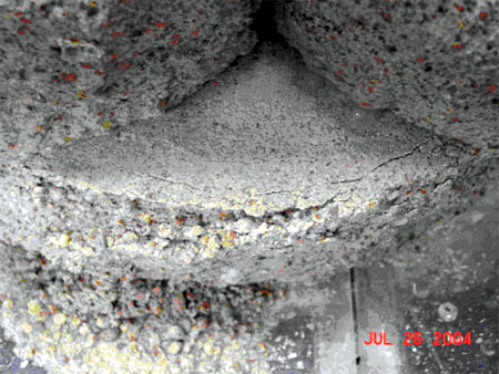
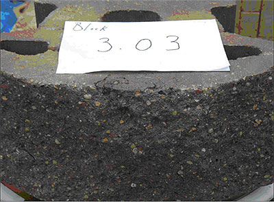
During field inspection, split face delaminations can mislead an inspector to attribute this feature as environmental damage or deterioration of the SRW unit. This confusion is enhanced by the fact that such features occur at the split surface of SRW units, which is also the surface in direct contact with the environment. During actual freezing conditions, water can seep into the space between the delamination and the SRW unit and expand upon freezing, thereby "jacking" the delaminated piece out of position (figure 47). Figure 48 shows a detached delamination under frost conditions. This mechanism may thus be interpreted as being frost-related damage during routine field inspection. One way that split face delaminations can be distinguished from other forms of damage is by the nature of the cracked and/or broken off residues. As shown in the previous sections, delaminated pieces tend to be thin and slender sections on the SRW split surface. On the other hand, frost degradation typically consists of crumbly material which appears in addition to cracking in the units, as shown in figure 49. Another point of distinction involves the quantity of fractured material. While split face delaminations tend to occur as single and isolated pieces, frost damaged material usually appears as more than one broken piece.
As for testing SRW units in the laboratory, perhaps the most critical issue with split face delaminations concerns the inclusion of these loose pieces in test specimens. While these delaminations are commonly observed on the surface of units as thin shallow pieces, it is not improbable that the cracks penetrate deeper into the units. Figure 50 shows a section through the split face of an SRW unit that was shipped directly from a manufacturer to Cornell without previous exposure in the field. The size of the cracked section is approximately 130 mm long (5.12 inches) and up to 20 mm deep (0.79 inch), and it is also possible that microcracks exist in the vicinity of the main crack shown. The concern is that, if a laboratory technician extracted specimens from the split face region of a unit containing these delaminations, results from tests (e.g., strength, absorption, freeze-thaw resistance) conducted on these specimens will be misleading. To prevent this, the technician must thoroughly inspect test specimens for cracks or loose pieces prior to testing them. If loose pieces are only prevalent on the specimen surface, these pieces can pried off; however, if the specimen is cracked, the cracked portions must be trimmed off from the specimen by saw-cutting; otherwise the test specimen should be discarded and another one extracted from the parent unit. An alternate and more reliable solution is to entirely avoid extracting samples from the split face region and sample from a different surface such as those shown by the dashed lines in figure 50a. Avoiding the extraction of specimens from the split face is currently a requirement in ASTM C 1262 (2003) as mentioned in section 4.2.1 of this chapter.
4.2.4 Recommendations for SamplingAs mentioned in 4.2.1, two different approaches to sampling could be taken depending on the intended purpose of the tests (to evaluate production methods and/or mix designs or to qualify units for projects). In either approach, the overall goal is to select units representative of the "lot" from which they are sampled and extract specimens representative of these units. Recommendations are offered in this section for specimen sampling. While these recommendations are intended for ASTM C 1262 (2003) freeze-thaw test specimens, they also apply to sampling for ASTM C 140 (2000) tests. 4.2.4.1 Sampling of SRW Units
It is understood that many laboratories in the industry employ this sampling technique for freeze-thaw test specimens (personal communications, NCMA, May 2005).
4.2.4.2 Extracting Specimens From SRW Units
There are occasions when specimens shorter than the actual height of the SRW unit may be required. For instance, 150-mm-(6-inch-) long specimens need to be extracted from 200-mm- (8-inch-) tall units. Such situations could arise where available container sizes pose a constraint, or if the performance of 200 mm (8 inches) units were to be compared to that of 150-mm (6-inch) units using specimens of similar dimensions. Since the specimen is now shorter than the unit height, material along the full height of the unit will no longer be represented within each specimen. Representation thus needs to be done over several specimens. A recommended approach to attain full height representation of the unit is shown in figure 53 where three specimens of required length X are extracted from a unit of height H at different positions so that their combined result reflects all layers equally. It is noted that the rightmost specimen shown in this figure actually comprises two halves, which is permitted under ASTM C 1262 (the two halves are "tested as and considered as a single specimen," Clause 7.1.4). When tested as a single specimen, these two halves must be tested using the same container size as the other full specimens (i.e., those shown on the left and middle in figure 53). The goal is to maintain the same (mass of test solution) relative to (mass of specimen) in each test container. It is noted that if shorter specimens are sampled in the manner shown in figure 53, it must be ensured that the total test area of all specimens in a set be within the range of total test area of all specimens as per ASTM C 1262 (2003). ASTM C 1262 (2003) requires five replicate test specimens with test area of 161 to 225 squared centimeters (cm2) (25 to 35 squared inches (inch2)) each. This adds up to 805 to 1125 cm2 (125 to 175 inch2) of test area per set. If specimens with an area of 150 by 75 mm (6 by 3 inches) are needed (test area of 113 cm2 (18 inch2)), nine specimens shall be sampled and tested (for a total area of 1013 cm2 (162 inch2). The reason for using nine specimens is because, as shown in figure 53, a set of three specimens is required to represent the face uniformly, and hence, only multiples of three-specimen sets can preserve this uniform representation. In the same manner that ASTM C 1262 (2003) requires five specimens extracted from five separate units, smaller specimens (1, 2 or 3 shown in figure 54) should also be extracted from separate units. Another important consideration regarding specimen extraction is that the actual size and shape of specimens cut from SRW units dictates the size and shape of container to be used (subject to the required clearance of surrounding test solution in ASTM C 1262 (2003)). The size and shape of container in turn influences the total number of containers that can be fit in a given shelf in freezer, which then influences the freezer air cooling pattern as discussed later in this chapter.
4.2.4.3 General Laboratory Practice
4.2.4.4 Other Research
4.3 VARIABILITY IN FREEZE-THAW EQUIPMENT USED IN ASTM C 1262 (2003)The previous section (section 4.2) discussed sources of test variability that could arise from specimen sampling, and a set of recommendations was provided to reduce this risk. Now, given that a population of similar specimens (similar geometry, mass, and properties) has been procured for freeze-thaw testing, the next question that arises is: how certain can a laboratory be that each and every specimen in this population is exposed to the ASTM C 1262 (2003) temperature-time (T-t) requirements during freezing? This section briefly addresses this issue by first exploring the extent of spatial variability in temperature that can exist within freezers, the significance of this variability, and recommended solutions to manage this variability. More thorough coverage of this technical issue can be found in Chan (2006) and Hance (2005). The clauses in ASTM C 1262 (2003) relevant to freezer equipment and to the freeze-thaw cycle follow:
These requirements are illustrated in the freezer-air cooling curve (T-t response) shown in figure 67 where various terms are defined. Cold soak is the time period during which the air temperature is between −18 °C ± 5 °C (0° ± 10 °F), and Clause 8.2.1 requires that cold soak be maintained for 4 to 5 hours. The cooling ramp is the portion of the cooling curve between the point at which the temperature starts falling until it reaches -18 °C ± 5 °C (0° ± 10 °F). ASTM C 1262 (2003) has no requirements for this cooling ramp. Together, the cooling ramp and cold soak comprise what is shown as the cooling branch of the curve. Similarly, on the warming side, the warm soak is the time period during which the air temperature is between 24 °C ± 5 °C (75 °F ± 10 °F); the warming ramp is the portion of the curve between the end of cold soak and the start of warm soak. While ASTM C 1262 (2003) requires the warm soak to be between 2.5 and 96 hours, it states no requirement on the warming ramp. Together, the warming ramp and warm soak comprise what is shown as the warming branch of the curve.
Strict interpretation of the ASTM C 1262 (2003) clauses shown above suggests that the T-t conditions stated in Clause 8.2.1 must prevail throughout the chamber during freezing and the conditions in Clause 8.2.2 must exist around the specimens during thawing. This is reasonable if uniformity in exposure conditions is to be maintained among all specimens. However, as discussed in detail in Chan (2006) and Hance (2005) and briefly in the remainder of this section, freezer air cooling curves can vary from location to location inside a freezer, which affects specimen exposure. Such variation is influenced by, and can be partially controlled by the manner in which freezers are operated. 4.3.1 Comparison Between Different FreezersThree different types of freezers were evaluated for internal temperature characteristics as briefly described in this section. The first was a chest freezer (figures 68 and 69) that can typically be purchased from appliance stores. This type of freezer cools the air within the freezer through its walls, and there is minimal air movement within the enclosed air space. Thus, high temperature gradients are likely inside this type of freezer. Since there are no automated temperature controls in these freezers, freeze-thaw cycling needs to be done manually (i.e., freezing by placing specimens into freezers and thawing by removing specimens from freezer and placing in laboratory air). Four such freezers were available for this study.
The second type of freezer was a walk-in environmental chamber (figures 70 through 72). Unlike the chest freezers, the walk-in freezer has ceiling mounted, fan-driven cooling and heating units that circulate conditioned air throughout the chamber, thereby promoting more uniform air temperature distribution. It operates at 2400 watts and has a cooling capacity of 0.13 watts per liter (watts/L) of freezer volume. This freezer has a programmable control device into which specified cooling and warming T-t profiles can be input and thus, continuous freeze-thaw cycles can be run without human intervention. The third type of freezer was a cabinet freezer commonly used in testing laboratories. This freezer, shown in figure 73, is also equipped with cooling and heating units which are programmable to allow uninterrupted freeze-thaw cycling. Fans are also built into the unit to move air through the cabin for better air temperature distribution. This freezer operates at 5200 watts with a cooling capacity of 9.8 watts/L of freezer volume.
For each freezer shown in figures 68-74, the temperature distributions throughout the chamber were accurately recorded while conducting test trials following ASTM C 1262 (2003). For each freezer, different tests were performed with varying numbers of test samples, up to the maximum sample number shown in table 2, which provides additional information on the freezers used in the study as documented by Hance (2005).
4.3.1.1 Chest FreezerIn his thesis, Hance (2005) showed results of experiments carried out to determine the internal temperature variation in a chest freezer containing six ASTM C 1262 (2003) specimens. A wooden frame was built onto which 18 calibrated thermocouples were mounted to measure temperature inside the freezer at various locations (figure 75). These thermocouples were placed at a distance of about 25 to 50 mm (1 to 2 inches) from the interior wall surface.
Figure 76 shows the T-t response in which the large spread in internal temperatures is shown. Hance's analysis of these temperatures was based on the ASTM C 1262-98 version which specifies a target cold soak temperature range of −17 °C ± 5 °C (−12 to −22 °C). A similar analysis is shown here but using the ASTM C 1262-98ε1 version which specifies a target cold soak temperature range of −18 °C ± 5 °C (−13 to −23°C) (this is also the version used throughout this FHWA project.) Based on the average temperature Tavg, cold soak started at 0.9 hours when Tavg reached −13 °C (8.6 °F) and ended at 4.9 hours for a 4-hour cold soak period (the minimum recommended in ASTM C 1262, (2003)) at Tavg of −16.6 °C (12.2 °F). At the start of cold soak, the range between minimum and maximum measured temperatures was 6 °C (42.8 °F), and this range gradually decreased to 4.2 °C (39.6 °F) after 4 hours of cold soak. Figure 77 shows the standard deviation (σ) of the temperature measurements as a function of time, where it is seen that standard deviation gradually decreased with increasing soak time (hovering in the vicinity of 1.5 °C (34.7 °F)). The temperature variations for this chest freezer are summarized in table 3. At the start of cold soak, approximately half of the temperature measurements are warmer than -13 °C (8.6 °F), while the other half are colder than -13 °C (8.6 °F). To increase the proportion of locations below -13 °C (8.6 °F), the temperature recorded at a single, random location (Trandom) must therefore be colder than -13 °C (8.6 °F). Assuming that the temperature inside the freezer follows a normal distribution (with mean Tavg and standard deviation σ), the value of Trandom must be such that: -13 °C = Trandom + 1.645σ, to ensure that 95 percent of the temperature measurements are below -13 °C. Thus, Trandom = -15.5°C (4.2 °F) Equation 2 -13 °C = Trandom + 2.325σ, to ensure that 99 percent of the temperature measurements are below -13 °C. Thus, Trandom = 16.5 °C (2.3 °F) Equation 3 [The above expressions are based on the standard normal distribution in which 95 percent of measurements is below a value of T95 percent = Tavg + 1.645σ while 99 percent of measurements is below a value of T99 percent = Tavg + 2.326σ (Miller and Freund, 1985). The aim here is to determine Tavg such that T95 percent and T99 percent are equal to −13 °C (8.6 °F). An average value of σ = 1.5°C (4.2 °F) over the cold soak duration was used in these calculations]. The values of Trandom calculated above indicate that due to variability in freezer internal temperature, the spot location must record an increasingly cooler temperature than -13 °C (8.6 °F) to ensure that most measured locations (95 and 99 percent considered) meet the -13 °C (8.6 °F) requirement.
* Based on Avg. ± 2σ, where σ is about 1.5°C over the duration of the cold soak period. 4.3.1.2 Walk-in Environmental ChamberSpatial temperature variability in the 18-m3 (630-ft3) walk-in chamber was evaluated by Hance (2005) using a similar approach. Eighteen calibrated thermocouples were located throughout the interior of this chamber as shown in figure 78. Evaluations were carried out at specimen quantities of 2, 20, 40, 60, 80, and 100 specimens. (Hance pointed out, however, that from a cooling capacity standpoint, 80 specimens appeared to be a reasonable upper limit for testing in this chamber). To illustrate the temperature variations in this chamber, results from the 60 specimen tests are shown in figures 79 and 80. Figure 79 shows the T-t response from the various thermocouples where it is observed that the band of curves was tighter than that obtained in the chest freezer. Again, based on average temperature, a 4-hour cold soak started at 4.3 hours with Tavg at -13 °C (8.6 °F) and ended at 8.3 hours with Tavg at -14.6 °C (5.7 °F). The range between minimum and maximum measured temperatures was 2.6 °C (4.7 °F) at start of cold soak and 1.6 °C (2.9 °F) at the end of the 4-hour cold soak. These parameters are summarized in table 4. The σ-t response is shown in figure 80. During cold soak, this parameter remained at about 0.4 °C (compared to 1.5 °C for the chest freezer). During the warming ramp, values of the standard deviation were higher likely due to nonuniform temperature conditions resulting from the introduction of warm air (from the heaters) to an already cold environment.
* Based on Avg. ± 2σ, where σ is about 0.4°C over the duration of the cold soak period. Compared to the chest freezer, the walk-in freezer exhibited more uniform temperature distribution, as indicated by the smaller standard deviation over the duration of the cold soak period (0.4 °C (32.7 °F) in walk-in freezer versus 1.5 °C (34.7 °F) in the chest freezer). This reduced temperature variation in the walk-in chamber was probably related to better air circulation imparted by the fans. As with the chest freezer however, due to variability in freezer internal temperature, the temperature recorded at a single, random location (Trandom) must be colder than -13 °C (8.6 °F) to increase the proportion of measurements below -13 °C (8.6 °F). Assuming a normal distribution for the freezer internal temperature, the value of Trandom must be such that: -13 °C (8.6 °F) = Trandom + 1.645σ, to ensure that 95 percent of the temperature measurements are below -13 °C (8.6 °F). Thus, Trandom = -13.7°C (7.4 °F) Equation 4 -13 °C = Trandom + 2.326σ, to ensure that 99 percent of the temperature measurements are below -13 °C. Thus, Trandom = -16.5°C (2.3 °F) Equation 5 [The rational behind these expressions is similar to the ones shown previously for the chest freezer. An average value of σ = 0.4 °C over the cold soak duration was used in these calculations]. As seen, due to the lower variability, the walk-in chamber required less "overshooting" (that is targeting of a spot temperature measurement lower than -13 °C (8.6 °F) to ensure that most locations are below -13 °C (8.6 °F)) than the chest freezer. Figure 81 shows the average T-t plots for the freezer air with various numbers of specimens, where it is clearly seen that the performance of the freezer depends on the number of specimens. While the initial rate of temperature change was similar regardless of specimen quantity (at about 56 °C/hr or 100 °F/hr), the curves diverged by the end of the test. Further, with increasing quantities of specimens, the time to reach start of cold soak was substantially delayed. For instance, with 20 specimens, Tavg reached -13 °C (8.6 °F) at 2.0 hours, whereas with 40 specimens, Tavg reached -13 °C (8.6 °F) at 2.8 hours and with 80 specimens, Tavg reached -13 °C (8.6 °F) at 7.0 hours. This means that as the number of specimens is increased, total testing time is expected to increase, and the rates of freezing will decrease. The temperature variations for each of these tests are summarized in table 5, in which the following trends were observed:
The overall significance of these results is that, as expected, freezer performance is dependent on specimen quantity in an interactive manner. As the number of specimens change, freezer performance is affected, which modifies the exposure condition of the specimens themselves. This freezer-specimen interaction must be taken into consideration in testing and will be discussed further.
n.a. = data not available 4.3.1.3 Cabinet FreezerSpatial temperature variability in the 0.53 m3 (18.8 ft3) cabinet freezer was assessed by placing 23 calibrated thermocouples throughout the freezer cabin. Evaluation of this freezer was carried out as part of the NCMA Foundation Study. At the time the freezer was received, four shelves were available, as shown in figure 74. Thermocouples were placed at each corner and the center of each shelf, as shown in figure 82. These thermocouples were typically located at about 25 mm (1 inch) above the shelf level. In addition, thermocouples were placed near the ceiling and the floor of the cabin, as well as adjacent to the freezer internal sensors. In total, 23 thermocouples were employed, and their locations are illustrated in figures 82 and 83.
Evaluations were carried out using 0, 18 and 28 specimens. To illustrate the internal temperature variations, results from the 28 specimen tests are shown here. This was also the number of specimens tested in the NCMA study. Figure 84 shows the T-t response from the thermocouples where it is observed that the band of curves was tighter than that obtained in the chest freezer but not as tight as the one obtained with the walk-in chamber, especially at the onset of cold soak. Based on average temperature, a 4-hour cold soak started at 1.9 hours with Tavg at -13 °C (8.6 °F) and ended at 4.9 hours with Tavg at -18.3 °C (-0.9 °F). The range between minimum and maximum measured temperatures were 3.2 °C (5.8 °F) at start of cold soak and 1.4 °C (2.5 °F) at end of the 4-hour cold soak. These parameters are summarized in table 6. The standard deviation-t response is shown in figure 85 where the standard deviation is seen to gradually decrease from approximately 0.8 °C to 0.3 °C (33.4 °F to 32.5 °F) from start to end of cold soak (compared to almost constant values of about 0.4 °C (32.7 °F) in the walk-in freezer and 1.5 °C (34.7 °F) in the chest freezer). As with the walk-in freezer, values of standard deviation increased during warming ramp. As with the chest and walk-in freezers, due to variability in freezer internal temperature, the temperature recorded at a single, random location (Trandom) must be colder than -13 °C (8.6 °F) to increase the proportion of measurements below -13 °C (8.6 °F).
* Based on Avg. ± 2σ, where σ averages about 0.6°C over the duration of the cold soak period. Assuming a normal distribution for the freezer internal temperature, the value of Trandom must be such that: -13 °C = Trandom + 1.6456σ, to ensure that 95 percent of the temperature measurements are below -13 °C (8.6 °F). Thus, Trandom = -14.0°C (6.8 °F) Equation 6 -13 °C = Trandom + 2.326σ, to ensure that 99 percent of the temperature measurements are below -13 °C (8.6 °F). Thus, Trandom = -14.4°C (6.1 °F) Equation 7 As seen, the "overshooting" (that is the targeting of a spot temperature measurement lower than -13 °C (8.6 °F) to ensure that most locations are below -13 °C (8.6 °F)) is intermediate between that of the chest and walk-in freezers. Knowing the locations of these thermocouples allowed mapping of the temperature inside the cabinet freezer to detect patterns within the freezer. This was done by selecting a time from the T-t record (3.5 hours arbitrarily selected), ranking the available temperatures at this time in order from coldest to warmest and splitting all the locations into six groups of three or four locations per group. These groups were then labeled from 1 at the coldest spots to 6 at the warmest spots. The result of this mapping is shown in figure 86 in which the overall coldest and warmest spots are also identified. The coldest locations generally were in the front part of the freezer (i.e., near the door) and on the higher shelves (including the ceiling), while the warmest locations were toward the back of the freezer in the lowest shelves (including the floor). The coldest overall location was right at the location of the freezer's built-in temperature sensor that is used to control the freezer cycles. This sensor is located near the fan. The warmest overall location was at the back of the bottommost shelf. This pattern of temperature distribution generally coincided with the flow of air within the chamber, illustrated in figure 87. As shown, the air coming out from the fan is the coldest air and reaches the top shelf and freezer front locations first. On the other hand, the back locations in the lower shelves are more or less sheltered, and as such, experience the warmest temperatures. The freezer's internal control sensors, positioned at the fan exit, were exposed to the coldest temperatures within the chamber. The T-t trace for this location is shown by the dark line in figure 84. This has important implications for test control as will be discussed later.
The effect of the number of specimens is seen in figure 88 showing the average T-t plots for the freezer air for 0, 18 and 28 specimens. Unlike the walk-in chamber, the initial rate of temperature change depended on specimen quantity from 61 °C/hr (110 °F/hr) with no specimens, to 27 °C/hr (49 °F/hr) with 28 specimens. The times required for Tavg to reach -13 °C (8.6 °F) were 0.7, 1.5 and 1.9 hours for 0, 18 and 28 specimens, respectively. The temperature variations for each of these tests are summarized in table 7. It is interesting that temperature variability at the start of cold soak in the cabinet freezer, even without specimens in it, was larger than that observed in the walk-in chamber. The 95 percent confidence range was 3.4 °C (38.1 °F) for the cabinet freezer with 0 specimens and 1.6 °C for the walk-in freezer with 60 specimens. Although the reason for the larger variability observed in the cabinet freezer at start of cold soak is unclear, it is suspected that at this time (start of cold soak when Tavg reaches -13 °C (8.6 °F)), the cabinet freezer was still experiencing rapid temperature drops (see figure 89) and a stable, more uniform air distribution throughout the freezer had not yet been reached. Once in the cold soak zone at more stable temperatures, variability decreased. Overall, increasing the number of specimens increased variability.
n.a. = data not available 4.3.1.4 Recommendations To Reduce Freezer Internal VariabilityAs seen from the previous sections, each of the freezers evaluated was capable of complying with ASTM C 1262 (2003) requirements, although the shapes of the T-t responses were quite distinct from freezer to freezer. Results of ASTM C 1262 (2003) tests conducted on specimens in different freezers (Haisler, 2004) showed that these kinds of shifts in T-t response (shown in figure 88) can have a very significant influence on specimen performance. The focus in this section is on how internal variability within a freezer can affect compliance with the test standard, and more importantly, how one can modify the freezer, specimen storage, or freezer controls to meet compliance with ASTM C 1262 (2003) and to provide consistent exposure conditions for all the samples contained in the freezer. Below are some recommendations for modifying ASTM C 1262 (2003) to meet these objectives. It is evident that cold and warm spots exist within each freezer. Specimens that remain in these cold and warm spots can conceivably be subjected to different numbers (and types) of freeze-thaw cycles and exhibit different durabilities. One way to minimize discrepancies in exposure conditions is to move samples periodically during the course, which is currently specified in ASTM C 1262 (2003):
Based on these clauses, specimens tested to 100 cycles would only be rotated four times through the entire duration of the test. Moreover, Clause 8.2.5 only mentions sample rotation in the vertical direction of the freezer. Hence, if a specimen is placed on the back side of the freezer, it is possible for it to remain on the back side through 100 cycles with the only difference being the shelf level. Similarly, there could also be specimens near the front of the freezer through the entire test. It is thus recommended that specimen rotation occur at intervals shorter than 25 cycles (say every 10 cycles), and that rotation be not only carried out in the vertical direction, but also within a shelf (e.g., front and back). This approach would allow for more uniform exposure of all specimens over 100 cycles. As demonstrated earlier for the walk-in and cabinet freezers, the T-t characteristics in these freezers varied when loaded with different quantities of specimens. This variation is as expected due to the different thermal mass associated with different specimen quantities and due to the way that specimen loading may influence interval air flow and convective heat transfer to or from any given specimen. Variations in specimen quantities, however, could arise due to a number of possible reasons, which include (but are not limited to) laboratory testing demand and schedules, specimen or container size constraints, or the gradual removal of specimens that are considered failed. On the issue of specimen and container size constraints, various possibilities exist which could ultimately result in different specimen quantities, with associated changes in T-t characteristics within the freezer. A simple but effective recommendation to address this issue is to standardize the container size to be used for ASTM C 1262 (2003) testing. Removal of failed specimens (e.g., mass loss exceeded specification limit) during the course of a test also changes the total number of specimens in the freezer and thus changes the exposure for the balance of the specimens. While such situations are clearly dealt with in ASTM C 666 (2004) for rapid freeze-thaw of ordinary concretes, ASTM C 1262 (2003) has no provision for this. ASTM C 666 (2004) covers this situation as follows: "Whenever a specimen is removed because of failure, replace it for the remainder of the test by a dummy specimen," (Clause 8.3, ASTM C 666, 2004). It is recommended that ASTM C 1262 (2003) adopt a similar provision and require that a failed specimen, upon removal from the chamber, be replaced by a "dummy" specimen to prevent fluctuations in the total mass inside the freezer during the course of a test. Overall, it is seen that total specimen quantity in the freezer can vary for a number of reasons, which alters the temperature environment inside the freezer. This in turn changes the exposure conditions of the specimen themselves. As such, it is important that laboratories conducting freeze-thaw tests survey their freezers before conducting tests, to identify these variations and the extent to which temperatures may be distributed in the freezer. Knowledge of this temperature variability should then be employed to plan tests cycles, the results of which can be used to optimize the testing regime for that given freezer. Complete details on this approach are provided in Chan (2006). This approach requires a test cycle to be run on a given freezer (with a given number of test specimens) with temperature monitored throughout the chamber, from which T-t and standard deviation-t curves can be generated. A reliability-based approach is then taken to optimize the control of the freezer to minimize locations within the freezer that are undercooled or overcooled, in other words to minimize the proportion of noncompliant locations within the freezer. This approach, which makes use of graphical reliability (R) curves, is described in appendix A, where it appears as an annex to a new proposed version of ASTM C 1262 (2003) based on the findings of this project. Additional information, including sample calculations, can be found in chapter 4 of Chan (2006). It should be noted that this approach of performing trial tests and statistically optimizing actual tests based on these results has already been applied to the NCMA-funded study and other ongoing projects. It must also be emphasized that R-curves portray a specific interaction between the freezer and specimens. A given freezer loaded with a certain quantity of specimens of a particular size, mass and arrangement inside the freezer will possess a uniquely characteristic R-curve. Changing any of these variables will alter the form of the curve. Finally, R-curves cannot be determined a priori but must be determined individually for each freezer and specimen configuration. 4.4 CHARACTERISTICS OF THE FREEZE-THAW CYCLESection 4.3 focused on evaluating temperature variability inside a freezer during a typical freeze-thaw cycle. The objective of this evaluation was to enable maximizing the number of locations in the freezer that were compliant with ASTM C 1262 (2003) cold soak requirements, which consists of maintaining the freezer air temperature at -18 °C ± 5 °C (0° ± 10 °F) for 4 to 5 hours (note that this is irrespective of how fast the freezer cooled to this condition). However, as shown in figure 89, the T-t response of the SRW specimen itself (as measured from sensors embedded in the specimen, figure 90) follows a path that is distinct from that of the freezer air. This section discusses the ice formation process and damage mechanisms as the specimen undergoes the various stages in a freeze-thaw cycle.
The work described in this section involved calorimetric methods to trace ice formation during freezing of plain water and 3 percent NaCl solution (salt as percentage of solution mass). The concept of freeze progress (or percent ice formed) was introduced to describe and quantify ice formation rates. Concentration changes in the salt solution during freezing were also examined. The work also includes the use of glass vials such as those shown in figures 91 through 94 to simulate freezing of solutions in saturated, confined spaces. Events taking place during freezing such as supercooling and expansion damage were traced along the T-t response of the solution. Other relevant aspects investigated included varying concentrations of salt solution, varying saturation levels, effect of cooling environment and estimation of ice pressures.
4.4.1 Significance of Freeze-Thaw CycleDifferences in the nature of the freeze-thaw environment can have an impact on specimen performance as evidenced from results obtained under this FHWA project and in the NCMA-funded project. In summary, for the NCMA study (described in detail in chapter 6 of Chan (2006)), specimens extracted from SRW units from a single production run were tested in two separate freezers: the walk-in chamber and the cabinet freezer, which were described earlier in this chapter. When tested according to ASTM C 140 (ASTM C 140, 2000), properties of the specimens evaluated in the two freezers differed by no more than 8 percent in their compressive strength (average 37 MPa (5,370 psi)) for specimens in walk-in chamber versus average 34 MPa (4,930 psi) for specimens in cabinet freezer), 2 percent in water absorption (127 versus 129 kg/m3) and 2 percent in oven-dry density (2230 versus 2210 kg/m3). Of the various test sets (labeled A to G) evaluated in the cabinet freezer, test set A specimens were similar to specimens tested in the walk-in freezer, which comprised nominal 200- by 100- by 32-mm-(8- by 4- by 1¼- inches-) size SRW coupons placed in 13 mm-(½ inch-) deep saline solution inside plastic containers of size 310 by 210 by 108 mm (12.3 by 8.3 by 4.3 inches), as shown in figures 95 and 96.
Figure 97 shows the percent mass loss (i.e., residues as percentage of initial specimen mass) through 200 cycles for 16 specimens in the walk-in freezer (lighter lines) and 4 specimens in test set A in the cabinet freezer (darker lines). The average mass loss of all specimens in the walk-in freezer, including the two specimens exhibiting sudden jumps in mass loss at about 80 and 100 cycles, was 0.2 percent after 100 cycles and 0.8 percent after 200 cycles. By contrast, the average mass loss of test set A specimens in the cabinet freezer was 0.4 percent after 100 cycles and 4.4 percent after 200 cycles. Thus, mass loss between specimens in the two freezers differed by up to a factor of 2 after 100 cycles and a factor of 5.5 times after 200 cycles. Structural integrity of specimens was monitored by changes in the relative dynamic modulus (RDM) of the specimens using resonant frequency methods (ASTM C 215, 1997). Figure 98 shows RDM through 200 cycles for these same specimens. The average RDM for specimens in the walk-in freezer was about 100 percent after 100 cycles and 79 percent after 200 cycles. By contrast, the average RDM of test set A specimens in the cabinet freezer was about 93 percent after 100 cycles and 4 percent after 200 cycles.
As for the test environments in these two freezers, figure 99 shows freezer air T-t curves for typical cycles in the two freezers. Also shown are T-t curves for the solution surrounding instrumented specimens in the two freezers. Both freezer air cycles were fully compliant with ASTM C 1262 (2003) test method requirements. Specimens in the walk-in freezer were subjected to a cold soak period of 4.8 hours, whereas specimens in the cabinet freezer were subjected to a cold soak period of 4.5 hours. Each freezer reached a different minimum air temperature at the end of cold soak (-16.9 °C (1.6 °F) in walk-in and -18.5 °C (-1.3 °F) in cabinet). The curves in figure 99 are reproduced again in figures 100 to 102 together with rates of change of freezer air temperature and solution temperature. Differences can be discerned in the following areas:
A summary of the measured differences between the two freezers is provided in table 8. How these specific differences in freezer air and solution temperature translated to specimen performance is yet to be explored, although it is evident from the mass loss and RDM curves that disparities in the performance were obtained from specimens tested in these two environments. The following sections describe experimental work carried out with the objective of elucidating ice formation in specimens and how these link to their cooling curves and to the overall requirements of ASTM C 1262 (2003).
a obtained from the tangent to the curves at T = -13 °C 4.4.2 The Cooling CurveChan (2006) in chapter 2 of his dissertation, presented the cooling curve for water and salt solutions in general and discussed in a qualitative manner the various steps taking place during their freezing. This section describes attempts to establish a more quantitative and mechanistic perspective of the cooling curve used in ASTM C 1262 (2003). Findings from this investigation are first highlighted, followed by their application to the understanding of the response of freeze-thaw test specimens. 4.4.2.1 Ice Formation and RatesIce formation in plain water and in 3 percent NaCl solution was measured using a calorimetric approach. A so-called "coffee cup calorimeter" was used to determine ice formation in freezing liquids, namely plain water and 3 percent NaCl solution. In this simple test, ice formation is measured by measuring heat changes inside the calorimeter which can in turn be related to ice quantities. Here, ice formation was traced by the parameter freeze progress (FP) which was defined as FP = mass of ice/mass of initial liquid x 100 percent. FP was traced as a function of temperature and time, which enabled plotting this parameter along the cooling (T-t) curves of these liquids. These results are shown in figure 103 for plain water and figure 104 for 3 percent NaCl solution. Note that in the cooling curve for 3 percent NaCl solution, the freezing plateau was not as well-defined as it was for plain water. This is due to the freeze concentration process, whereby the yet unfrozen portion in a saline solution becomes increasingly concentrated in salts as ice crystallizes out of solution during freezing (Sahagian and Goff, 1996). This process leads to the continuously decreasing freezing point of the solution which contrasts with the constant freezing point of water (at T of about 0 °C (32 °F)). As such, for the saline solution, a quasi‑freezing plateau was defined as the region between supercooling and the region of maximum curvature (between t = 250 to 300 min). Figures 103 and 104 show FP-t curves; while figures 105 and 106 show the rates of ice formation (i.e., d(FP)/dt). The main conclusions drawn from this work follow:
Another result from this work was plots of FP versus T which are shown in figure 107 for water and 3 percent NaCl solution. Here, it is seen that for water most of the ice formed at about 0 °C (32 °F) while for the saline solution, ice formation was accompanied by reductions in temperature. At -18 °C (0.4 °F) which is the target cold soak temperature in ASTM C 1262 (2003), there was still about 15 percent unfrozen solution. The significance of this on ASTM C 1262 (2003) testing will be discussed later in this chapter.
4.4.2.2 Changes in Concentration for Saline SolutionIn addition to ice formation, changes in the concentration of the unfrozen solution were also measured and traced along the cooling curve for the 3 percent NaCl solution, as shown in figure 108. It is noted that beyond about 165 minutes cooling, measuring this concentration experimentally was difficult due to increased ice formation. Also plotted in figure 108 are concentration versus time values based on tabulated data in the CRC Handbook of Chemistry and Physics (CRC, 1988). It is seen here that at approximately halfway through the quasi-freezing plateau, the concentration of the unfrozen portion of the solution had risen up to about 5 percent from the initial 3 percent. Near the end of this quasi-plateau, this concentration was about four times the initial value. By the time the temperature of the solution was at the ASTM C 1262 (2003) cold soak target of -18°C (0°F), this concentration was at about six times the initial value. Figure 109 shows the rate of concentration change plotted together with the rate of ice formation (from figures 105 and 106). It is evident that ice formed most rapidly during the quasi-freezing plateau, whereas the concentration of the unfrozen solution increased most rapidly near the end of this plateau.
4.4.2.3 Damage PointVarious experiments were conducted in which water or saline solution-filled vials were utilized to model saturated, confined spaces. Expansion damage, as manifested by fracture of the vials, was detected using three different methods:
For circuit resistance tests, typical results are shown in figures 113 through 118 for different setups of the vials (water-filled unconfined vial, water half-filled unconfined vial, and water‑filled mortar confined vial). In each case, thermocouples at two locations (top and bottom, see figure 92) were used to register the T-t response, and two wire loops were also setup at the approximate heights of the thermocouples. Figures 113 through118 show results for T-t response from the thermocouples as well as the resistance versus time response from the circuit. In all cases shown, at least one of the circuits broke near the end of the freezing plateau on the cooling curve. These points of rupture are also shown in the figures. These observations suggested that expansion damage in the vials occurred near the end of the freezing plateau, just before the temperature dropped further.
For strain gage tests, results for vials filled with water and 3 percent NaCl solution are shown in figures 119 through 122. The T-t curves from thermocouples in the liquid are shown as well as the strain gage response along the circumferential direction at vial midheight. In both cases, there was substantial activity recorded along the freezing plateau. For water, the strain peaked sharply at the start of the plateau and reached another peak again just before the end of the plateau. This agrees with the result obtained using the circuit resistance method in which rupture was also detected near the end of the plateau. Figure 120 shows the multiple failure locations on the vial (cracking along the vial body and breakage of the cap). For 3 percent NaCl solution, the strain reached two consecutive peaks also at the start of the plateau and gradually subsided. Multiple fracturing along the vial was also observed (figure 122).
For the direct observation tests, results for vials filed with water and 3 percent NaCl solution are shown in figures 123 and 124, respectively, where the cooling curves are shown along with photos of the vial condition at various points on the curves. In these tests, it was observed that immediately after supercooling (at 50 mins in both figures 123 and 124), a cloudy phase propagated from the top to the bottom of the vial, filling the vial entirely with a crystalline network, as shown by figures 123b and 124b. This propagation event lasted anywhere from 5 to 10 seconds and marked the start of the freezing plateau. The plain water vial burst at around the 60-minute mark from start of cooling, and as shown in figure 123c, the bottom thermocouple was left exposed to freezer air, while the top thermocouple was still surrounded with ice. This is likely why the bottom thermocouple recorded a sudden drop in temperature, while the top thermocouple continued recording a full freezing plateau. As for timing, the "explosion" occurred at approximately one-quarter of the way into the freezing plateau as recorded by the top thermocouple. Similarly, the saline solution vial burst at around the 65-minute mark which corresponded to approximately one-third of the way into the quasi-freezing plateau as recorded by the bottom thermocouple (figure 124).
In summary, these vial tests, despite being performed via different approaches, all pointed toward the fact that expansion damage of the vials could occur at any point in the freezing plateau of the cooling curve. While the circuit resistance method indicated that rupture occurred at the end of the plateau, the other two methods suggested there were volume changes including the possibility of damage at any point during the plateau. Nevertheless, it appeared that in all cases, as long as a complete freezing plateau was observed in these tests, expansion damage would have occurred in the vials. Damage was not observed after the freezing plateau. 4.4.2.4 Connection to Freeze-Thaw Test SpecimensCooling curves of ASTM C 1262 (2003) test specimens were monitored using thermocouples embedded in the specimens themselves. For each specimen of size 76 by 229 by 33 mm (3 by 9 by 1.3 inches), three thermocouples were grouted into predrilled holes in the specimens as shown in figures 125 and 126. The specimens were then placed in plastic containers that were 152 by 305 by 90 mm (6 by 12 by 3.5 inches), and the containers were subsequently filled with water to the 13-mm (½ inch-) level (figures 127 and 128). These instrumented specimens were subjected to ASTM C 1262 (2003) freeze-thaw cycles while their internal temperatures were monitored. An example of the response measured by one of these specimens was shown earlier in figure 89.
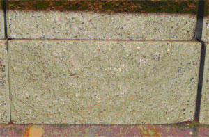
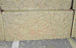
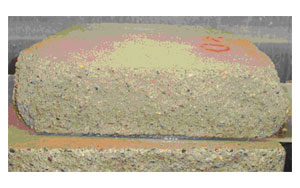
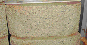
Figure 129 shows cooling curves for two instrumented SRW specimens that differed in their internal structure and material properties. SRW mix A was characterized by higher volume fraction of paste and lower volume fraction of total voids (air and compaction) compared to SRW mix B, as shown on the photos in figures 130 and 131.
From the cooling curves of these specimens, it is seen that while pore water in mix B specimen froze at approximately the same temperature as the bulk water surrounding the specimen, pore water in mix A specimen had a slightly lower freezing point. In both cases, however, the cooling curve of the pore liquid in the specimens followed similar overall pattern as the cooling curve of the surrounding water as well as the liquids shown in preceding sections, which were characterized by a freezing plateau followed by a rapid descent in temperature. Based on our understanding of the processes occurring during freezing of liquids as presented earlier in this chapter, it is thus evident that various physical and chemical changes are taking place during freezing of solutions in the specimens. With this consideration, it also becomes apparent that specimens over a range of test conditions (e.g., specimens in different container sizes, in different locations in a freezer, in different freezers, and even from cycle to cycle) can exhibit different cooling curves and possibly different extent of damage. The following parts show how specimen cooling curves may, however, vary under different conditions. I. Varying volume of surrounding water Specimen cooling curves were obtained by Hance (2005) in the walk-in freezer using the same instrumented specimens as those described above, but with varying volumes of surrounding water. These tests were conducted with the freezer loaded with a total of 40 specimens, and the results are reproduced in figure 132. The curve corresponding to a specimen immersed in water at the standard ASTM C 1262 (2003) depth of 13 mm (½ inch) is shown by the curve labeled "As spec." Variations to this condition involved changing the water volume by adding or removing 50 or 100 mL (1.7 to 3.4 fl oz) from the container, resulting in the other curves shown in the figure. It is interesting to note that while the initial cooling portions of the curves (prior to the freezing plateau) were similar in all cases, the lengths of freezing plateau and the shapes of the curve following the freezing plateau were dissimilar in each case. Increasing the volume of surrounding water had the primary effect of prolonging the freezing plateau. For the various curves in figure 132, the length of the freezing plateau was estimated using the method shown in figure 133, and these results together with other key parameters are summarized in table 9. It appears that in general, for every 50 mL (1.7 fl oz) increase in water, the freezing plateau was lengthened by about ½ hour. Another observation from these results is a difference in the final specimen temperature at the end of the cold soak periods. For every 50 mL (1.7 fl oz) increase in water, the specimen temperature increased by 0.7 to 2.2 °C (1.3 to 4.0 °F) after a 4-hour cold soak and by 0.1 to 0.7 °C (0.2 to 1.3 °F) after a 5-hour cold soak.
This suggests that the specimen temperature is less sensitive to variations in surrounding water volume at a 5-hour cold soak (i.e., more time is required to remove the additional latent heat of fusion from the extra water.) However, at a given water volume, the difference in specimen temperature between 4 and 5 hours of cold soak ranged from 1.4 °C (2.5 °F) for the -100 mL (-3.4 fl oz) case to 5.5 °C (9.9 °F) for the +100 mL (3.4 fl oz) case. The slopes of the post freezing plateau part of the cooling curve were similar in all cases. II. Varying container size In a separate test, Hance varied the container size which correspondingly led to variations in water volume. Two container sizes were used: the same one as above (152 by 305 by 90 mm (6 by 12 by 3.5 inches)) and a smaller one (135 by 241 by 76 mm (5¼ by 9½ by 3 inches)). Both container sizes yielded clearances (specimen-to-edge of container distance) that were compliant with ASTM C 1262 (2003). The specimen cooling curves are shown in figure 134 where it is also seen that variations in this curve resulted from changes in container size. Key parameters for this comparison are shown in table 10.
III. Varying specimen quantities in a freezer Section 4.3.1.2 demonstrated that the freezer air temperature in the walk-in chamber varied with increasing specimen quantities ranging from 2 to 100 specimens. In those tests, instrumented specimens were also placed in the freezer to obtain the specimen cooling curves under these conditions. The results are shown in figure 135 in which the freezer air temperature curves are reproduced. It is seen that substantial variations in actual specimen cooling response ensued by varying the number of specimens in the chamber. Differences were seen in various parts of the cooling curve as summarized in table 11. Overall, specimen initial cooling rates were lower and final specimen temperatures were higher as the total specimen quantity increased. It is also noted that while freezer air temperatures did not drop significantly lower in going from a 4-hour cold soak to a 5-hour cold soak, specimen temperatures dropped an additional 1 °C (2 °F) during this extra hour. Whether this additional 1 °C (2 °F) has any impact on the damage process in the specimens is not clear. The freezer air temperature curves shown in figure 136 for 2, 20, 40 and 60 specimens were compliant with ASTM C 1262 (2003) requirements. For 80 and 100 specimens, data collection was discontinued before the 4-hour cold soak was reached, but in these cases, the freezer air response could have been "made compliant" to ASTM C 1262 (2003) by simply extending the cooling time to the necessary time to achieve 4-hour cold soak (as long as it is below -13°C (8.6 °F).
IV. Single location repeatability The instrumented specimen was also used for tests inside the chest freezer presented in section 4.3.1.1. In one particular set of tests, the specimen was subjected to repeated freeze-thaw cycles in a single location of the freezer to determine the single-location repeatability of this particular freezer (note that for the chest freezer, cycling had to be performed manually). The specimen was placed in the lower back corner of the freezer as illustrated in Figure 138. The resulting freezer air and specimen cooling curves for seven cycles are shown in Figure 139. The overall range of freezer air temperatures among all seven cycles was about 1 °C (2 °F) during the time period of 2 to 4 hours. In general, the specimen cooling curves were more or less similar, particularly during initial cool down and over the freezing plateau. The main difference was in the cooling region beyond the freezing plateaus. Of all seven cycles, the shortest one had a freezer air cooling branch that was 6.4 hours long while the longest one had a cooling branch that was 6.9 hours long. The specimen temperature reached -9.2 °C (15.4 °F) in the shortest cycle and -10.2 °C (13.6 °F) in the longest cycle. As mentioned before, it is not certain whether this extra 1 °C (1.8 °F) drop in specimen temperature is significant as far as specimen damage is concerned.
V. Different freezers With data from instrumented specimen tests in the walk-in and chest freezers, it is also possible to compare responses in two different freezers. Figure 140 shows the specimen cooling curves under these two freezers. While both freezers were capable of complying with ASTM C 1262 (2003), some differences were observed in the overall shape of the air and specimen cooling curves. The specimen cooling curves, however, showed similar initial cool down rates (about 14 °C/hr (25 °F/hr)) and lengths of freezing plateaus (2.9 hours in chest freezer and 3.1 hours in walk-in freezer). The specimen temperatures at the end of a 4-hour cold soak were also similar (-11.4 °C (11.5 °F) in the chest freezer and -10.9 °C (12.4 °F) in the walk-in freezer).
In general, it is seen that variations in the exposure conditions of specimens can influence the actual cooling curve of the specimens themselves. One key finding from these studies is the fact that complying with ASTM C 1262 (2003) freezer air T-t requirements does not necessarily guarantee similar cooling responses in specimens. It appears that variations in the surrounding water volume and in the number of specimens inside the freezer caused the largest discrepancy among cooling curves. Variations in container size also caused differences in the cooling curve, but this is probably due to the variation in surrounding water volume. Specimens in the chest freezer loaded with 6 specimen's portrayed similar response to specimens in the walk-in freezer loaded with 40 specimens. This shows it is possible to attain similar specimen cooling responses even between separate freezers. Similarly, repeatability within a single location in the chest freezer was reasonable. Note that in all specimen cooling curves considered above, the freezing plateau was completely traversed by the end of a 4-hour cold soak. Accordingly, from the standpoint of inducing expansion damage, it appears that the current 4-hour minimum cold soak in the ASTM C 1262 (2003) is adequate to fulfill this purpose. It is interesting to note that the cold soak requirement in an earlier version of this test method (ASTM C 1262-94) consisted of maintaining the chamber air temperature at -17.8 to -9.4 °C (0 to 15 °F) for 3.5 to 4.5 hours (for similar size specimens and containers). Using the curves in figure 129 as example, cold soak would start after 1 hour from start of test (based on the 1994 version of ASTM C 1262) and end after 4.5 hours cooling time at the earliest. However, after 4.5 hours, this specimen was still undergoing its freezing plateau and thus, full expansion damage potential is likely not realized. Hence, the cold soak requirement of 3.5 hours starting at -9.4 °C (15 °F) as required in the previous version of ASTM C 1262 (2003) is not adequate. This discussion has applied observations from the vial tests to pore liquid in the specimens. While this approach may be valid for large pores where water exists in bulk state, it may not be valid in smaller pores where the surface effects become critical. One result of such effects is the depression of freezing point when water freezes in increasingly smaller pores. Figures 140 and 142 show various relationships from the literature between pore size and temperature at which ice formation is possible. Figure 141 shows that for pore radii above 50 nm (2x10⁻⁶ inches), freezing temperature of fresh water is close to 0 °C (32 °F). Figure 142 shows theoretical freezing points above -5 °C (23 °F) for pore sizes greater than 10 nm (2.5 X 10⁻⁷ in.) or 25 nm (1 X 10⁻⁶ inches), depending on the assumption regarding the controlling interface in the pores (solid-liquid or liquid-vapor) (Marchand et al., 1995). For SRW mixes, compaction voids can account for up to 25 percent of the volume fraction of the material and the sizes of these voids can range from fractions of a millimeter to several millimeters (see figures 130 and 131 for example). Freezing of water in these pores is therefore probably close to freezing in the bulk state. For smaller capillary and gel pores in the paste fraction of SRW mixes, the freezing point is likely to be depressed and to follow relationships similar to those shown in figures 141 and 142.
Figure 141. Graph. Relationship between size of pores and freezing point from Pigeon and Pleau (1995).
Figure 142. Graph. Relationship between size of pores and freezing point from Marchand et al. (1995). Tf = (9/5) * Tc + 32 {Tf = Fahrenheit, Tc = Celsius} In saline solution, aside from ice formation, a concentration change in the unfrozen portion of the solution was also measured that increased most rapidly near the end of the freezing plateau. Concentration gradients lead to osmotic pressures, which have been cited in the literature as a primary mechanism for deicing salt scaling (Harnik et al., 1980). Even without the presence of salts, Powers has pointed out that concentration differences due to freeze concentration of the pore solution can induce osmotic pressures large enough to damage the concrete (Powers, 1975). If osmotic effects due to concentration changes were significant, these effects are likely to become increasingly important after ice has started forming (once the freezing plateau has started) and throughout the duration of cold soak. For testing purposes, to minimize differences that may be incurred by different laboratories due to different cold soak durations, an upper limit on the cold soak period of the test is therefore required. The currently specified 5 hours in ASTM C 1262 (2003) may thus fulfill this purpose. 4.4.2.5 Rates of Temperature ChangeIn the same manner in which rates of temperature change were determined for freezer air and solution temperatures in section 4.4.1, rates of temperature change were also determined for an SRW specimen from its cooling curve. Temperature data from a specimen tested in the walk-in freezer loaded with 40 specimens (labeled "As spec." in figure 132) were used to calculate these rates. Figure 143 shows the T-t curve for freezer air, water surrounding specimen and specimen itself for one cycle (top graph). Directly below this graph are the rates of temperature change for the solution and specimen temperature, followed by a graph showing the difference in temperature between center of specimen and freezer air (ΔT = Tfreezer air - Tspecimen). From the dT/dt graphs, it is seen that the specimen and its surrounding water underwent similar patterns in terms in their temperature change rates, although the specimen dT/dt response appeared to lag that of the water. Despite the lag, peak dT/dt values for the specimen were not far from the peak dT/dt values for the water at the following times:
Larger differences in peak rates of temperature change were observed at these times:
Tf = (9/5) * Tc + 32 {Tf = Fahrenheit, Tc = Celsius}
Thus, overall, it appears that peak rates in either cooling or warming of the specimen were similar to the corresponding rates in the surrounding water. This similarity in rates only happened when both specimen and surrounding water were at similar initial temperatures (24 °C (75 °F) during initial cooling and -16 °C (3 °F) during warming after cold soak). The peak rates of cooling in the specimen also occurred at approximately the same time as for water. However, when being cooled or warmed from different starting temperatures such as at the end of freezing plateaus or during thaw plateaus, the peak rates in temperature change differed for both specimen and surrounding water. Figure 143 shows the temperature difference between center of specimen and freezer air, ΔT. This graph shows that the largest temperature gradients occurred during initial cool down (from 0 to 1 hour) and for about 2-3 hours after end of cold soak. 4.4.3 Other Aspects Relevant to the ASTM C 1262 (2003) Test MethodWhile the 4 to 5 hour cold soak requirement in ASTM C 1262 (2003) may be adequate to induce damage in specimens as shown previously, there are other aspects of the freeze-thaw cycle that must also be considered. These are discussed here. 4.4.3.1 Concept of Frozen SolidDespite setting a 5 hour maximum limit on cold soak, ASTM C 1262 (2003) permits extending the cold soak if the water (or solution) surrounding the specimens does not appear to be frozen solid. This is stated in Clause 8.2.1: Periodically, at the end of a freezing cycle, open the containers and visually inspect the specimens to determine if all the water surrounding the specimen is frozen solid. If not, extend the length of the freezing cycle to ensure that all water is frozen solid. From this statement, it appears that the interpretation of what constitutes "frozen solid" is left up to the discretion of the test operator. Figures 144 and 145 show pictures of two specimens tested in 3 percent NaCl solution and removed from the freezer after a 4.5-hour cold soak. While the solution around figure 144 appeared to be completely frozen, the solution around the specimen figure 145 exhibited wet spots over it. Thus, while the specimen in figure 144 may be considered to have reached frozen solid conditions, the one in figure 145 may not be and consequently kept in the freezer for additional cold soak time. This decision thus affects the actual exposure condition of specimens. This issue is better understood by examining the FP versus T curves shown earlier in figure 107. A solution with initial 3 percent NaCl concentration attains an FP of about 85 percent by the time its temperature reaches the target cold soak temperature of -18°C (0°F). This means there is still approximately 15 percent unfrozen solution that could either become entrapped within the ice or reside on the surface of the solution giving the impression that the solution is not yet frozen solid. Given that complete freezing of an NaCl solution is not possible until eutectic temperature is reached (-21°C (-6°F)), it is recommended that cold soak be limited to the current 5 hour maximum and that the condition of frozen solid be removed from the test standard.
4.4.3.2 Temperature ToleranceThe current allowable cold soak temperature in ASTM C 1262 (2003) is -18 ± 5 °C (0° ± 10 °F). An inspection of the NaCl-H2O phase diagram reveals that the eutectic point for this system exists at temperature of -21°C (-6 °F) which is the lowest temperature at which a solution will remain completely liquid. Below this point, solid ice and NaCl·2H2O crystals are the thermodynamically stable phases which means that salts will crystallize from the remaining solution (Van Vlack, 1967). Although the extent to which NaCl crystallization may damage the concrete under these conditions was not investigated here, damaging pressures caused by salt crystallization from supersaturated conditions are well documented in the literature (Charola, 2000; Scherer, 2004; and Pigeon and Pleau, 1995). It is therefore recommended that unless otherwise demonstrated, the minimum allowable temperature during cold soak shall remain above -21 °C (-6 °F). Recall that earlier in this chapter, it was mentioned that at cold soak temperatures above approximately -14 °C (7 °F), reliabilities of 100 percent were unattainable in the walk-in freezer. This issue in conjunction with the eutectic point issue mentioned above provide compelling reasons to tighten the allowable cold soak range from -18 ± 5 °C (0° ± 10 °F) to -18 ± 3 °C (0° ± 5 °F). This is in fact the allowable temperature range specified in ASTM C 672 (2004) for deicing salt scaling resistance of concrete. 4.4.3.3 Cooling Rates and Target Cold Soak TemperaturesWhile a target cold soak temperature range and duration are specified in ASTM C 1262 (2003), cooling rates are currently not specified (i.e., how fast the temperature drops from warm to cold soak). Cooling rates have been cited in the literature as being significant, especially for large pore systems (Petersson, 1999 and Scherer, 1993). Cooling rate is also a parameter in Powers' classical hydraulic pressure theory to estimate pressures in concretes (Powers, 1949). One important outcome from the vial tests described earlier was the comparison of vial performance under two freezers with different cooling environments. Vials similar to those described in section 4.4.2.3 were prepared but instead of being filled to capacity, were only filled halfway. Figures 146 through 149 show the T-t response for these two vials, as well as pictures of them. While the vial tested in the chest freezer fractured (figure 147), the vial tested in the walk-in chamber did not exhibit signs of damage (figure 149). Table 12 shows a summary of relevant temperature parameters to compare the exposure conditions of these two vials. Generally, water in the chest freezer cooled about 1.2 to 1.6 times faster, and ice formed about 1.5 times faster than in the walk-in freezer. Distinct modes of ice formation were also observed in these two vials. Figure 150 and 151 show views of a half-full vial after 30 and 40 minutes in the chest freezer. The growth of ice at the air-water interface is clearly seen. After 40 minutes (figure 151), the surface was hard enough to resist the weight of the screwdriver shown. In essence, an "ice plug" appears to have formed at the top of the liquid column and the yet unfrozen liquid below this plug was thus "enclosed." These vials were damaged as shown by the cracks in figure 147. On the other hand, as shown in figure 149, ice formed from within the liquid column in the walk-in freezer, and a rise in the column was observed. No damage was observed in this vial. Cooling rates may have played a role in determining whether or not damage occurred in these vials. Given that cooling rates may play a role in inducing damage, actual specimen cooling rates are now presented and compared to cooling rates in other freeze-thaw test methods. For the specimen cooling curves presented in section 4.4.2.4, cooling rates were calculated by taking the difference between the specimen temperature after 4-hour cold soak and 20 °C (reference initial value) and dividing this difference by the time taken for the specimen to drop from 20 °C to the 4-hour cold soak point. This is expressed in equation 9:
Note that this cooling rate is different from those shown in section 4.4.2.4 that corresponded to initial cooling rates from 20 °C to 0 °C. The reason for calculating cooling rates in the manner shown in equation 9 is to enable comparison of this parameter with other existing freeze-thaw test methods. Specimen cooling rates obtained using equation 9 is summarized in table 13.
a Evaluated as the slope of water T-t curve between about 20 and 0°C for the bottom thermocouple. b Evaluated in the manner shown in figures 146 through 149. c Rate = volume of water / length of freezing plateau, assuming 90 percent of the total water freezes during the plateau.
*From initial 20 °C (68 °F) to temperature at end of 4-hour cold soak. As a point of reference, ASTM C 666 (2004) for rapid freeze-thaw testing of ordinary concretes specifies the specimen T-t regime shown in figure 152. The graph shown is for ASTM C 666 (2004), Procedure A which consists of freezing and thawing in water. For the target values shown in figure 152, average cooling rates of 5.9 to 14.8 °C/hr (11 to 27 °F/hr). It is seen that in general, the cooling rate of the ASTM C 1262 (2003) specimens presented in section 4.4.2.3 was near the lower end of the ASTM C 666 (2004) range.
Another example of a specified specimen cooling curve is given by the European cube test for surface scaling and beam test for internal damage (Siebel, 1995). The specified cooling curve envelopes for these tests are shown in figure 153. Cooling curves for the specimens tested in the chest and walk-in freezers (specifically those shown in figure 140) are also plotted for comparison. It generally appears that the cooling curves obtained for the ASTM C 1262 (2003) test specimens followed more closely those of the cube test designed for surface scaling tests, except for the specimen temperature at end of cold soak.
4.4.3.4 Degree of SaturationThe above observations on half-full vial tests also suggested that partially saturated systems may be damaged during freezing. For cementitious systems, it has been traditionally reported in the literature that damage can occur if the capillary pores are filled with water above a critical saturation of 91.7 percent (Cordon, 1966). The observations from these tests, however, suggest that damage can occur at saturation levels well below the critical value depending on the cooling environment. This has important implications for ASTM C 1262 (2003) that involves freezing and thawing of partially immersed specimens (figure 154). Local moisture content profiles could vary among specimens due to variations in capillary rise caused by sample microstructural differences, changes in ambient conditions, or even specimen geometry. It is recommended that further research be carried out to compare the performance between fully saturated and partially saturated specimens and to determine the extent that saturation effects may have on test variability.
4.4.3.5 Warming RateWarming rates also are not currently specified in ASTM C 1262 (2003). Warming rates, especially while the ice is still solid (i.e., from the minimum test temperature to the point before ice melts), may contribute to damage in the cementitious material. This is because ice has a coefficient of thermal expansion of about 50 x 10-6 /°C (25 x 10-6 /°F) (Michel, 1978) which is approximately five times the value of about 10 x 10-6 /°C (5 x 10⁻⁶ /°F) for concrete (Neville, 1996). As such, during rapid temperature rise, the differential expansion between the ice and concrete can generate internal stresses. This potential damage mechanism has also been discussed in other references (Kaufmann, 2002; Kukko, 1992; Venečanin, 1984). 4.4.4 Summary—Implications for ASTM C 1262 (2003)From the results and observations of the experimental work described in this chapter, it is apparent that a number of damage-inducing processes can take place during the freezing and thawing of specimens. It is key that specimens tested under different conditions such as different containers, container sizes, locations within a freezer or freezers undergo similar exposure if they are to experience similar forms and levels of damage. It has been demonstrated that variations in surrounding water volume and total quantity of specimens in the freezer can have an impact on the specimen cooling curves. The issue of surrounding water volume suggests that this parameter should be fixed to prevent variations arising from fluctuations in this parameter. The impact of specimen quantity was reflected by markedly different freezer air and specimen cooling curves for varying loads of specimens. For each load of specimens, however, ASTM C 1262 (2003) freezer air T-t requirements were still met which indicates that these requirements must be revised and tightened to avoid variations such as the ones presented here. The current cold soak requirement of 4 to 5 hours at -18 ± 5 °C (0° ± 10 °F) appears adequate for inducing expansion damage due to ice formation in specimens. Extensions beyond the 5 hour maximum based on operator interpretations of frozen solid conditions (as is currently the case in Clause 8.2.1) are not recommended. As far as the cold soak length is concerned, as shown in tables 9, 10, and 11, one consequence of allowing a 1-hour window in cold soak times is that the minimum specimen temperature will reach different values. This discrepancy was particularly pronounced in the comparison of specimens with different volumes of surrounding water. Tightening the allowable cold soak time to 4.5 to 5 hours may thus be justified on this basis, although further investigation would be required to determine the effect of cold soak length on specimen performance and whether variations in cold soak length contribute to variability of test results. Moreover, modifying the length of cold soak may influence the manner in which freezers are operated. As far as temperature tolerance is concerned, it is also recommended that this be tightened for the reasons discussed in section 4.4.3.2. Specifying target cold soak temperature ranges and durations still does not address the rate at which the freezer air temperature must cool down. For the freezers and thermal loads evaluated at Cornell, rates during initial cooling of freezer air have ranged as follows (based on the time taken for this temperature to drop from about 24 to -13 °C (75.2 to 8.6 °F):
20 specimens: 19 °C/hr (33 °F/hr) 40 specimens: 13 °C/hr (24 °F/hr) 60 specimens: 9 °C/hr (15 °F/hr) 80 specimens: 5 °C/hr (10 °F/hr)
28 specimens: 19 °C/hr (35 °F/hr) Similarly, warming rates are not specified in ASTM C 1262 (2003). For tests at Cornell, freezer air warming rates have ranged as follows (based on the time taken for this temperature to rise from its value at end of cold soak to 19 °C (66 °F):
(specimens were physically removed from freezer and placed in laboratory air environment)
20 specimens: 37 °C/hr (67 °F/hr) 40 specimens: 37 °C/hr (67 °F/hr) 60 specimens: 34 °C/hr (61 °F/hr) 80 specimens: 34 °C/hr (61 °F/hr)
28 specimens: 53 °C/hr (95 °F/hr) As was shown in section 4.4.1 (describing selected results from the NCMA study), test specimens exhibited discrepancies in performance despite being tested in two freezer environments whose air temperatures complied with ASTM C 1262 (2003). Differences in the actual rates of cooling and warming were observed between the two freezers. Further research is vital to investigate the impact of cooling and warming rates on specimen performance. There are two parts to this issue. One is the cooling and warming rates of freezer air which is the control medium currently used in ASTM C 1262 (2003) and is easiest to measure in a testing laboratory. The other is cooling and warming rates of specimens themselves, which reflect actual mechanisms taking place in the material. Whether specifying a complete freezer air T-t curve—which would include cooling rate and duration, cold soak temperature and duration, warming rate and duration, and warm soak temperature and duration—necessarily yields consistent specimen cooling curves remains to be explored. It was noted from figure 140 that specimens placed in the chest and walk-in freezers exhibited similar cooling curves despite differences in the freezer air response, which shows promise in the attainment of similar specimen cooling curves. It is also noted that the specification of complete freezer air T-t characteristics may entail specification of particular types and performance of freezers, as well as the total number of specimens (actual test specimens and dummy specimens) in the freezer at any given time, as is currently done in ASTM C 666 (2004). 4.5 SYNOPSIS OF NCMA STUDYAs described in section 4.1, toward the end of this FHWA-funded project, the research team for this project performed additional, focused research funded by NCMA. Although this work was not formally linked to this FHWA project, it did build on the key findings of this project, and given the synergy between the two studies, it is logical and efficient to consider the findings from both projects when making recommendations and giving guidance to SHAs on freeze-thaw durability of SRW blocks. This section provides a brief summary of the main objectives and findings of the NCMA project that were performed at Cornell University. For more complete details of the NCMA-funded efforts, refer to chapter 6 of Chan's 2006 dissertation. Overall, the NCMA funded project addressed the following general issues:
The NCMA research project was divided into two main parts: variability test series and performance criteria (PC) test series. The scope of each of these parts is only briefly described in this section; the reader is directed to Chan (2006) for full details on the study. The specific findings from the NCMA study are not presented in this section (for conciseness), but the key findings were taken into account when compiling the main conclusions for this report (chapter 5) and for providing guidance to SHAs on how to ensure long-term durability of SRW blocks through prudent and scientifically-based testing (see appendix A for new version of ASTM C 1262 (2003) based on the findings of both the FHWA and NCMA studies). 4.5.1 Variability Test SeriesFollowing up on potential sources of variability in ASTM C 1262 (2003) already discussed in this chapter, the NCMA study focused on the following issues:
This series was intended to evaluate the effect of variations within the ASTM C 1262 (2003) by varying specimen and container sizes to the extremes of ASTM C 1262 (2003) tolerances. The tests in this series used 3 percent NaCl, and after every tenth cycle, the condition of the specimens was assessed by the following methods:
The above tests assess different forms of specimen damage (note that ASTM C 1262 (2003) only relies on mass loss for damage assessment). While mass loss and scaling rating are sensitive to external forms of damage (i.e., loss of material from specimen surfaces), resonant frequency and pulse velocity are more sensitive to changes in specimen integrity (such as internal cracking). The evaluation of specimens using these various techniques allows observing how different forms of damage evolve with increasing freeze-thaw cycles and more importantly, enables comparing what certain forms of damage such as mass loss mean in terms of other forms of damage, such as specimen integrity, as measured from resonant frequency changes. 4.5.2 Performance Criteria (PC) Test SeriesIn addition to assessing specimen condition using mass loss, resonant frequency, ultrasonic pulse velocity and visual scaling rating, PC specimens were also tested for their modulus of rupture (MoR). The MoR is a useful mechanical property which characterizes the tensile capacity of the material. The primary objective of the PC Series was to correlate MoR to the other measured properties listed earlier. For these specimens, all measurements except for MoR were conducted after every 10th freeze-thaw cycle. MoR tests were conducted on selected specimens at different mass loss levels so as to obtain a spread of MoR values over the mass loss range of 0 to 2 percent. 4.5.3 Significance of NCMA Project FindingsThis NCMA study was quite comprehensive in the breadth of testing that was performed and the range of issues that were investigated. It is beyond the scope of this report to synthesize and present the conclusions and recommendations that emanated from this work. However, in chapter 4, some of the key findings of the NCMA study are presented, primarily those that are most relevant and have been integrated into guidance for SHAs currently testing, specifying, and using SRWs. 4.6 FROST DURABILITY INDICES FOR SRW UNITSThis section describes comprehensive testing of a range of SRW units obtained from commercial sources in North America. The main goal of this part of the project was to assess the durability of the units, using ASTM C 1262 (2003) (in water and 3 percent NaCl), and to identify which material characteristics, such as paste content, absorption, and microstructure, most relate to frost resistance. A main goal was to determine if one could measure select SRW block properties (other than frost resistance) and then predict frost resistance (as per ASTM C 1262 (2003)), based on these material properties. Briefly , the objective was to attempt to identify a frost durability index or frost durability indices that can be used as surrogate predictors for durability. It should be noted that this work was based on the standard ASTM C 1262 (2003) test method that existed at the time that this project was initiated, and as such, the testing described herein did not incorporate the various suggestions for improvements that were described throughout this chapter. The work presented herein was based entirely on research conducted under this FHWA project, and this summary draws from the following publications, especially the first one listed, developed under this project:
4.6.1 BackgroundThe frost durability of SRW blocks is most commonly assessed by using ASTM C 1262 (2003), which involves freeze-thaw cycling of specimens in either water or 3 percent NaCl solution up to a prescribed number of cycles (typically 100). At this point, the condition of the specimens is evaluated, and their mass loss is determined and compared to specifications such as ASTM C 1372 (2003). The overall test may require up to 2 to 3 months before completion due to the time required for carrying out each full cycle, periodic specimen inspection, and logistical factors. As a result, quicker assessments of freeze-thaw durability, such as the use of frost durability indices, may gain wider popularity in this industry. In ordinary concretes, the spacing factor as determined by the methods of ASTM C 457 (2004) has been commonly used as an indicator of frost resistance, with a transition between durable and nondurable concretes existing somewhere between a spacing factor of 200 to 250 μm (0.008 to 0.010 inch) (Hover, 1994). Although ASTM C 457 (2004) tests can be performed on SRW concretes, the applicability of the spacing factor to SRW concretes has been questioned. This is in part due to the different nature of voids comprising SRW concretes compared to those in ordinary concretes (Marchand et al., 1998). The NCMA has suggested an index to assess frost resistance of SRW concretes based on simple parameters such as compressive strength, 24-hour absorption and unit weight of SRW units (Thomas, 2003). These parameters, obtained from ASTM C 140 (2000) testing, are combined in the following manner:
Units possessing larger values of I were generally shown to have better likelihood of meeting test specifications (typically, maximum 1 percent mass loss after 100 cycles). For instance, for freeze-thaw tests in water, only about 10 percent of specimens with I < 58 MPa1/2 (700 psi1/2) met specifications. However, 43 percent of specimens with I of about 133 MPa1/2 (1,600 psi1/2) and 71 percent of specimens with I > 208 MPa1/2 (2,500 psi1/2) met specifications (Thomas, 2003). In a review of previous research work, Hance determined that frost durability of dry concrete products correlated well with cement content (Hance, 2005). Minimum cement contents of 252 to 395 kg/m3 (425 to 665 lbs/yd3) were generally required for frost resistance in water and 320 to 380 kg/m3 (540 to 640 lbs/yd3) for frost resistance in the presence of deicing salts. This section describes analyses of common SRW material characteristics as frost durability indices. Properties considered included those obtained from common tests such as ASTM C 140 (compressive strength, absorption and unit weight) and ASTM C 642 (2002) (boiled absorption and volume of permeable voids). In addition, characteristics obtained from microscopy analyses (ASTM C 457 (2004)) were also evaluated. The utility of the NCMA index as a frost durability index was also assessed. 4.6.2 Databases of SRW Block Freeze-Thaw Performance and Material PropertiesAs part of this project, databases of ASTM C 1262 (2003) freeze-thaw mass loss and material characteristics properties from ASTM C 140, C 642 and C 457 tests were obtained for SRW units from 5 different manufacturers (labeled A to E). For manufacturers A to D, two different types of SRW units were evaluated: units that satisfied DOT specifications in the State of the project (henceforth called DOT units), and units that did not necessarily satisfy DOT specifications (called nDOT units). DOT units tended to be denser with lower amounts of compaction voids compared to nDOT unit. For manufacturer E, nDOT SRW wall and cap units were evaluated. Hence, a total of 10 different types of SRW units were evaluated. Table 14 shows the scope of ASTM C 1262 (2003) freeze-thaw tests conducted on these SRW units. For DOT and nDOT units from manufacturers A to D, tests were conducted in water and 3 percent NaCl solution inside two different types of temperature-controlled freezers: large walk-in freezer and Tenney freezer (a cabinet style freezer). For the units from manufacturer E, the tests were carried out inside a commercial chest freezer. These various types of freezers were all capable of meeting T-t requirements of ASTM C 1262 (2003). For manufacturers A to D units, five replicate specimens were tested per set, while for manufacturer E units, three replicate specimens were tested per set. The data available from these tests consisted of the percent mass loss after 100 cycles.
Table 15 shows a summary of the standard material property tests performed on the SRW units. The number of replicate specimens tested varied for each type of SRW unit and generally ranged from 3 to 12 specimens. With respect to the ASTM C 457 (ASTM, 2004) compositional parameters, the total (air and compaction) void and paste contents refer to the volumetric fraction of these phases as determined from microscopy examinations. Air and compaction voids were distinguished during the microscopy tests using the following decision rule: a compaction void was defined as a void in which less than three-fourths of its boundary was a paste-void interface, while an air void was defined as a void in which more than three-fourths of its boundary was a paste-void interface irrespective of shape of void as shown in figure 155. With respect to the ASTM C 457 (2004) air void parameters, the specific surface is defined as the boundary surface area of air voids divided by the volume of the voids; the spacing factor is the average half‑distance between two voids. It is noted that these air void parameters were developed for ordinary concretes in which spherical bubbles are assumed to exist. One of the aims of this study was to assess the applicability of these parameters (determined in the usual way for concretes) for SRW concretes.
a Total air and compaction void content.
Also, NCMA index (I) as in equation 10 Several other relationships were also explored without much success. This section only focuses on results obtained with the parameters shown above. 4.6.3 Synthesis of DataThe overall experimental program involved shared testing responsibilities between two laboratories. While the majority of freeze-thaw tests were conducted in one laboratory, the majority of material property testing was conducted in another laboratory. It was therefore deemed inadequate to directly correspond mass-loss values to material characteristics as single (x, y) data points for each of the various SRW mixes evaluated, given the fact that specimens for each of these tests were extracted from separate parent SRW units. Consequently, an alternate method of reducing the data was employed as shown in figure 156. Here, it is shown that for each type of SRW unit (e.g., manufacturer X DOT), there was a range of freeze-thaw mass-loss values from the three or five specimens tested in the set. Similarly, there was a range of values for a given material property from the various replicate specimens tested in the set (3 to 12 specimens). Hence, for this particular SRW unit, the mass loss versus property relationship could be represented by any point in the shaded box bound by the minimum and maximum mass-loss values in the ordinate and the minimum and maximum values of the material property in the abscissa. This set of data points bound by the shaded box was then reduced in one of two ways explained below.
As a first approach, the shaded box in figure 156 could be reduced to a single data point representing the geometrical centroid of the box for a particular manufacturer (figure 157). The use of centroids for this purpose was deemed reasonable for several reasons. First, various data sets consisted of only three to four data points which was not sufficient to fully describe a statistical distribution. For these particular sets, the centroid was used as an approximate representation of the region bound by the maximum and minimum values in each axes. For larger data sets (five or more data points), the data points appeared to be normally distributed as confirmed using the statistical test of normality, and the centroid was thus taken as a representation of the shaded box. This process could then be repeated for all other SRW unit types to produce a data series as shown in figure 157. Each data point in this series represented results for one type of SRW unit. The disadvantage of this method is that by using single data points, the significant scatter in the data is ignored.
A different approach to represent the shaded box of figure 156 was to focus on its boundary points. This method would take into account the range in test results and perhaps be more representative of the actual nature of the data. Hence, for a given SRW type, its mass loss versus property relationship would be represented by four points (figure 158). When repeated for all other SRW unit types, a series of data points representing the corners of all boxes would be produced as shown in figure 158. A data series constructed by either one of the methods shown in figure 157 or 158 provided a qualitative representation of the behavior of the variables considered. In addition, a relationship was fitted through the data points to obtain a quantitative interpretation of the dependence between variables. Curve fitting was performed using the software Table Curve 2D®, Version 4, from AISN Software Inc (copyright 1989-1996). In this program, the user has the option of choosing the types of equations to be fitted through the data points. The option Curve-Fit Simple Equations was selected for this study. The result of the analysis consisted of a listing of expressions ranked in order from highest to lowest correlation coefficient (R2). Typically, the equation with the highest R2 value was selected as being representative of the relationship between variables. These R2 values were also used to compare the correlation strength between the various material characteristics considered and mass loss from freeze-thaw testing. In addition to R2 values, standard errors were also obtained for each curve fit. Furthermore, from the above plots, it was possible to determine approximate threshold values of the material property above or below which the mass loss would exceed a mass-loss limit (e.g., 1 percent in ASTM C 1372(2003)). This concept is illustrated in figures 157 and 158.
4.6.4 Discussion of ASTM C 1262 (2003) (in Water) ResultsResults of the above analyses are shown in figures 159 to 184 for ASTM C 1262 (2003) freeze-thaw mass loss in water and the following material characteristics: figures 159 and 160, compressive strength; figures 161 and 162, 24-hour absorption; figures 163 and 164, unit weight; figures 165 and 166, NCMA index; figures 167 and 168, boiled absorption; figures 169 and 170, volume of permeable voids; figures 171 and 172, saturation coefficient; figures 173 and 174, total air and compaction voids content; figures 175 and 176, paste content; figures 177 and 178, paste-to-total-voids ratio; figures 179 and 180, specific surface; figures 181 and 182, spacing factor; and figures 183 and 184 spec surf/total voids content. In each pair of figures, one corresponds to data representation by boundary points while the other corresponds to data representation by centroids. With respect to the number of data points in each graph, it is noted that for units from manufacturers A to D, tests were carried out in two types of freezers, and as such, two sets of data per SRW unit type from these manufacturers were available. Hence, the total number of "boxes" in the upper graphs or "centroid" points in the lower graphs was equal to 18 (4 manufacturers (A to D) x 2 unit types (DOT and nDOT) x 2 freezers + manufacturer E x 2 unit types (wall and cap) x 1 freezer). From figures 159 to 184, the scatter in test results was evident by the size of the constructed boxes. This scatter was particularly evident for freeze-thaw mass-loss as reflected by the height of the boxes. Despite this scatter, trends in the data were generally discernable and as expected. For example, mass loss increased with increasing total voids content and absorption (24-hour and boiled) and with decreasing paste content and unit weight. Lower mass loss also corresponded to higher values of the NCMA index, which was in agreement with the trends reported by Thomas (2003). The decreasing mass loss with increasing specific surface was comparable to the trend expected for conventional concretes. As for spacing factor, the observed trend was actually opposite to that expected for ordinary concretes, where lower spacing factors are characteristic of systems with more closely spaced air voids and hence better frost durability. It is possible that this parameter cannot be applied to SRW concretes in the same manner as applied to ordinary concretes perhaps due to differences in the air void structure. Mass loss also decreased with increasing value in the parameter (spec. surf.) / (total voids volume). This parameter could be envisioned as the amount of surface area afforded per unit volume of voids. To supplement observations of trends in the data in these plots, curves were fit into the data series to provide a quantitative sense of these trends. The inset boxes in figures 159 to 184 show the expressions for the best-fit curves, along with their corresponding R2 and standard error values for each material property considered. (That these equations are only valid within the range of values of SRW unit characteristics covered by the test data sets.) It is apparent that these equations were generally of power or exponential form which suggested that the mass loss was fairly sensitive to the characteristics considered. This sensitivity can also be visually detected from the shape of the curves where the mass loss exhibited steep changes relative to most of the material characteristics. With respect to the R2 values, it is noted that these were generally fairly low (up to 0.33 for analysis with boundary points and up to 0.69 for analysis with centroids), which was likely due to the scatter in test data. These R2 values were nevertheless used as a comparative basis of the correlation strength among the various material characteristics evaluated. In addition to the above analysis that was conducted for all available mass-loss results, an additional set of analyses was carried out on subsets of the previous databases that had a maximum mass loss of 5 percent. This separate analysis was carried out because, in practice, for SRW mixture qualification, freeze-thaw tests may be discontinued as soon as test specimens exhibit a substantial amount of mass loss (several times greater than the maximum allowed by project specifications). This concept is illustrated in figure 185. Table 16 shows a summary of various characteristics evaluated ranked in order from highest to lowest R2 value for both analysis covering mass loss up to 100 percent and maximum 5 percent (ranking of these characteristics based on standard error yielded similar results). Here, it is seen that the paste-to-total-voids ratio consistently ranked among the top three in each form of analyses. Its components, paste content ranked in the top three in two of the four analysis, and total voids content ranked at the top in one of the analysis. These results demonstrate the significance of material compositional parameters on the durability of the SRW unit. The NCMA index ranked reasonably high (top three in two analysis cases and top five in another case), which was likely due to the correlation strength of the 24-hour absorption and to some extent, the unit weight. ASTM C 642 (2002) parameters were modest in their ranking, while ASTM C 457 (2004) air void parameters ranked in the lower third of all parameters considered. The observation that mass loss correlated better with paste content rather than strength was in agreement with the results from Ghafoori and Mathis (1998), where cement content showed highest correlation to mass loss and with the literature review findings of Hance (2005). The saturation coefficient, which is commonly used as frost criterion for clay or shale bricks (ASTM C 672), was not suitable for the SRW units evaluated in this study. Hence, it is evident that typical frost performance criteria for other types of porous materials (spacing factor for ordinary concretes and saturation coefficient for bricks) may not be equally applicable to SRW concretes.
* Notation: fm = compressive strength; 24A = 24-hour absorption; OD = oven-dry density; NCMA = NCMA index; BA = boiled absorption; VPV = volume of permeable voids; TV = total air and compaction void content; P = paste content; P/V = paste to total voids ratio; α = specific surface; L = spacing factor; α/TV= specific surface / total voids; SC = saturation coefficient It is noted that, despite the helpfulness of curve fits in providing a quantitative interpretation of these data series, the actual behavior of mass loss relative to material characteristics is probably best discerned from the nature of the data itself. For instance, from figures 159 to 184, it is evident that the constructed boxes resembled some form of step function, whereby mass loss could range from being negligible to almost 100 percent in the region to one side of a certain critical value of the material property, but be low (less than about 1.5 percent) on the other side of this critical value. As such, it is possible that threshold values in most of the material characteristics exist beyond which there is a greater likelihood of larger mass loss. For the particular SRW units evaluated, the threshold values are summarized in table 17. With respect to ASTM C 140 (2000) parameters, these threshold values would have satisfied the specification values of ASTM C 1372 (2003) (Comp. strength: 57 MPa (8,270 psi) threshold versus minimum 21 MPa (3,050 psi) spec., 24-hour absorption: 85 kg/m3 (5.3 pounds per cubic foot (pcf)) threshold versus maximum 208 kg/m3 (13 pcf) spec. for normal weight SRW units). With respect to ASTM C 457 air void parameters, the threshold value for specific surface (15 mm2/mm3 or 375 inch2/inch3) was found to be similar to those found for concretes of satisfactory frost resistance (16 mm2/mm3 or 400 inch2/inch3 in Neville (1996)). The threshold value for spacing factor (120 μm or 0.005 inch) differed from the maximum 200 to 250 μm (0.008 to 0.010 inch) values of frost durable concretes. In fact, these threshold values would not be comparable since the trend in mass loss relative to spacing factor appeared to be different for SRW concretes than for normal concretes.
4.6.5 Discussion of ASTM C 1262 (2003) (in 3 percent NaCl solution) ResultsFigures 186 and 187 show the mass loss versus paste-to-total-voids ratio plots for tests in 3 percent NaCl solution. Greater data scatter was observed in these tests, as evidenced by the longer boxes in the vertical direction. This implied it was possible for some specimens to significantly outperform other specimens obtained from the same SRW unit (same composition and manufacturer). Although the mass loss generally decreased with increasing paste-to-total-voids ratio similar to the trend observed in water, there were instances of units with relatively high paste-to-total-voids ratio that also showed significant mass loss. This observation occurred similarly for other material characteristics and indicates that units considered of high quality when in tested water may still display a substantial mass loss when tested in saline.
4.6.6 SummaryVarious common SRW concrete material characteristics were assessed for their potential as frost durability indices by evaluating their correlation to ASTM C 1262 (2003) freeze-thaw mass loss. Of all parameters considered, the paste-to-total-voids ratio exhibited the strongest correlation to freeze-thaw mass-loss in water. Its components, paste content and total voids content, also exhibited strong correlations demonstrating the importance of unit composition on frost durability. The NCMA index showed fair correlation to mass loss, which was likely attributed to the correlation strength of the 24-hour water absorption. The spacing factor and saturation coefficient displayed low correlation to mass loss implying that these parameters may not be applicable to SRW concretes in the same way that they apply to ordinary concretes and clay bricks respectively. The threshold compressive strength value was determined to be well above the minimum specification value, while the 24-hour water absorption was well below the maximum specification value. This implied that SRW units that barely meet standard specification for these material characteristics may not necessarily be guaranteed frost durability. Finally, it was demonstrated that trends and observations drawn from water tests may not be entirely applicable to saline solution tests due to the higher data scatter in saline tests. Units considered of high quality when tested in water may display substantial mass loss when tested in saline. 4.7 Synopsis of study on effects of alternative deicing salts on SRW block durabilityAs described in chapter 3, significant damage has only been observed for SRW blocks in the field when the blocks are exposed to high levels of both moisture and deicing salts (or fertilizer). The key role that deicing salts play in field damage seems to justify the need to include salts in freeze-thaw testing in the laboratory. A significant amount of laboratory work has already been described in this report that included the use of salt solution, and in each case, the salt used was 3 percent NaCl solution. However, in highway applications, it is becoming more common for alternative deicing salts to be used, especially MgCl2. To address this point, a comprehensive study was initiated under this FHWA project in which the durability of SRW blocks was assessed while exposed to four different deicing salts and one commercially available fertilizer. For conciseness, only a brief synopsis of this study is presented herein. Full details can be found in:
In this study, two different SRW concretes were subjected to freeze-thaw cycles (following ASTM C 1262 (2003)) and continuous warm immersion tests to determine possible chemical effects from the salts. The salts used in these tests included:
The results of the freeze-thaw testing are summarized in figure 188. At 3 percent concentration (by mass of solution), NaCl solution was the most detrimental of all salts evaluated under freeze-thaw conditions. Freeze-thaw mass loss of specimens tested in NaCl solution (about 85 percent after 100 cycles) was approximately twice that of specimens tested in all other salt solutions (30 to 50 percent) (compared to about 1 to 2 percent in plain water). It generally appeared that as the solution freeze-point depression (ΔTfr) increased, the number of cycles taken before reaching 1 percent mass loss decreased. It is worth noting the fertilizer solution used in the tests was capable of causing as much freeze-thaw damage as most other deicing salt solutions, which has important implications for SRWs in areas frequently exposed to fertilizing compounds. It is recommended that freeze-thaw tests also be performed with similar salts but at varying concentrations to achieve similar ΔTfr for all test solutions.
In tests involving continuous immersion in warm solutions, particles of mix A and B were damaged by solutions of both CMA and MgCl2, while no damage was detected in other salt solutions even after 15 months of immersion. 4.8 RESEARCH ON DEVELOPMENT OF MORE REALISTIC FREEZE-THAW TEST FOR SRW BLOCKSThis section describes research aimed at developing a new, more realistic approach to testing SRW blocks. It is intended to address some of the shortcomings of ASTM C 1262 (2003), such as issues with sampling (and inherent variability for specimens extracted from a given block), repeatability (or lack thereof), and applicability to real-world exposure conditions (due to overly severe conditions induced in ASTM C 1262 (2003)). With this in mind, research was initiated under this FHWA project to develop and assess a testing regime that would allow for the testing of full SRW units or multiple SRW units stacked in a given formation (including cap units on top) under simulated field conditions. By grouping the SRW blocks in a simulated wall setup, deterioration that replicates field conditions is more likely to occur because stresses or restraint caused by adjacent blocks and drainage typical of that found in the field can be simulated. Thus, a new test method that represents field conditions would be useful so that SHAs and manufacturers can better assess the freeze-thaw durability performance of SRW blocks. The research herein consisted of two testing phases: the first phase consisted of performing trial tests on smaller-scale SRW blocks and the second phase used the information from the first phase testing to develop a standard test to evaluate the freeze-thaw performance of larger-scale SRW blocks typically used in transportation infrastructure systems. 4.8.1 Phase I InvestigationA preliminary freeze-thaw test procedure was developed and testing performed to assess the freeze-thaw performance of smaller, commercially available SRW blocks. It was anticipated that these results would provide preliminary information for the Phase II test procedure. The Phase I tests were performed to identify and resolve issues with the initial setup design, identify key parameters of the experiment, and set standards for the Phase II procedure. The focus of developing this new test method was to replicate field environmental conditions as closely as practical by implementing slower temperature changing rates, longer temperature hold times, and spray exposure conditions instead of ponding. Equipment necessary for constructing the test setup included a programmable temperature-controlled environment, a spray system with cyclic capabilities, and a test chamber large enough to hold six to nine SRW blocks. The programmable, temperature-controlled chamber was able to control the temperature from −20 °C to 24 °C (−4 °F to 75 °F) and was able to ramp at least 0.55 °C (1 °F) per minute on the freezing cycle. The environmental chamber also incorporated a spray system for applying salt or fresh water solutions. A drawing of the exposure chamber used in this study is shown in figure 189. The overall dimensions of the chamber were 0.9 m wide by 1.8 m long by 1.5 m tall (3 ft by 6 ft by 5ft). The chamber support structure was built with a 51 mm (2 inch) angle iron frame to support the weight of the SRW blocks. The top and sides of the chamber were fixed with sheets of Plexiglas® to retain the spray solution during testing. The chamber was equipped with a drain system that recycled the solution. The spray system consisted of eight 6 mm (0.25 inch) stainless steel spray nozzles with 2 mm (0.081 inch) maximum free passage orifices and a 19 L (5 gal) per minute maximum flow rate to ensure complete coverage of the SRW block samples. The spray nozzles were attached to 9.5 mm (0.375 inch) stainless steel tubing that was fixed in the chamber. Four nozzles were positioned in front of the wall and four above the wall to ensure complete exposure to the test solution. A ball valve was placed before each set of nozzles to regulate the flow. A ¾ HP 316 stainless steel centrifugal pump was used to pump the solutions. This pump was controlled by electrical timers (mechanical timers can also be used) that enabled the pumps to turn on for 15‑minute intervals during the thaw cycle. A 49 L (13 gal) polypropylene reservoir was used to store the spray solution. A return line from the pump discharge was installed to prevent damage to the pump if the spray nozzles became blocked.
Four experiments were completed during the Phase I testing. The Phase I plan consisted of evaluating sets of 13 SRW blocks in each test. The temperature ramp rate, the temperature hold times, and the solution type were investigated in this phase. Table 18 provides an overview of the parameters investigated for each of the tests conducted.
NT = not tested To prepare the blocks for testing, the blocks were oven dried at 113 °C (235 °F) for 24 hours, labeled, and then weighed. These values were recorded as oven dry weights. After the weights were recorded the blocks were submerged in water until they reached saturation (typically after 48 hours). The blocks were then removed from the solution, surface dried, and these weights were recoded as original saturated weight. After these data were obtained, the blocks were stacked in the freeze-thaw chamber. The first three rows of blocks as shown in figure 190 (labeled A through L) were used for mass loss measurements. The top block, identified as Block M, was used for temperature measurements. The chamber temperature varied from −18 °C to 16 °C (0 °F to 60 °F). The temperature ramp rates were adjusted to achieve specified temperature changes in the blocks. The cycles consisted of the hold times shown in table 18.
To evaluate the internal temperature of the SRW blocks a 6.35-mm (0.25-inch) hole was drilled in the back of Block M to the center of the block. A Type J thermocouple was inserted into this hole and the hole was backfilled with approximately 25.4 mm (1 inch) of mortar made from a mixture of water, cement, and the block drill dust. The remaining hole was then filled with an insulating foam spray. The block temperature ramp rates and hold times were monitored to define the appropriate parameters for the actual test. The blocks were sprayed with solution (either NaCl solution or water) for 15 minutes prior to the start of the freeze cycle. The samples were exposed to 10 freeze-thaw cycles and then evaluated for freeze-thaw damage by visual inspection. These blocks were then saturated for at least 12 hours to restore any evaporated moisture during the testing. As already noted, the surface of the blocks was dried and the blocks were weighed after every 10 cycles. After weighing, the blocks were restacked in the chamber in the same order as the original stacking. Photographs of the blocks were obtained for a visual record, and the test cycle was repeated. Small commercial landscaping SRW blocks were procured for the Phase I testing. The typical dry weight of these blocks was 12 kg (26.5 lbs), and the dimensions of these blocks are shown in figure 191. All of the surfaces were relatively smooth except the front surface. The front surface consisted of a split face.
The freeze-thaw performance of the smaller SRW blocks was assessed by measuring the mass loss of the blocks (based on saturated weights) after the blocks were subjected to 10 freeze-thaw cycles. Figure 192 shows the weight loss for block samples from test 1 (ramp rate of 0.33 oC/min (0.6 oF/min) with 1 hour hold time sprayed with water). Figures 193 through 195 show the weight loss values for samples from test 2 (ramp rate of 0.18 oC/min (0.3 oF/min) with 1-hour hold time sprayed with 3 percent NaCl solution), test 3 (ramp rate of 0.33 oC/min (0.6 oF/min) with 1-hour hold time sprayed with 3 percent NaCl solution), and test 4 (ramp rate of 0.55 oC/min (1.0 oF/min) with 2-hour hold time sprayed with 3 percent NaCl solution), respectively.
It can be seen from figure 192 that samples exposed to water-spray exhibited limited weight loss after 100 freeze-thaw cycles, whereas several blocks exposed to the same ramp rates and hold times, but exposed to the 3 percent NaCl solution (figure 193) exhibited significant mass loss after 80 cycles. Three of the blocks in test 2 suffered severe deterioration and were considered to fail the test based on an arbitrary 5 percent mass loss criteria, and two other blocks showed significant distress as shown in figure 193. This clearly shows that the presence of salt increases the potential for damage, just as in the field and in ASTM C 1262 (2003), but it should be noted that not all the blocks showed significant damage in this test. Figures 193 through 195 show the influence of temperature ramp rates and temperature hold time on the freeze-thaw performance of small SRW blocks. Three samples exposed to Test 2 conditions (ramp rate of 0.18 °C/min (0.3 °F/min) failed before 100 freeze-thaw cycles. Four of the samples exposed to the Test 3 conditions (ramp rate of 0.33 °C/min (0.6 °F/min) failed before 100 freeze-thaw cycles. Although this tends to indicate that faster rates lead to more failures, because of the limited number of tests performed, only limited conclusions can be made. However, when evaluating the samples that were exposed to the Test 4 conditions (ramp rate of 0.55 °C/min (1.0 °F/min) with 2 hour hold time sprayed with 3 percent NaCl solution, seven small SRW blocks failed, indicating that the faster ramp rates and/or the longer hold time accelerated the freeze-thaw deterioration. The time for the cycling of the environment is approximately 1 hour. This time and the hold time are approximately 3 hours. As noted earlier, 2 to 3 hours are typically required to reach freezing conditions in the field. Although the test likely does freeze the sample in less time than that typical of field conditions, it is slower than the standard test procedure and likely better represents field conditions. Figures 196 and 197 show typical damage triggered by this test, with the manifestation of damage mimicking typical freeze-thaw distress observed in field situations.
Test 4, which included a ramp rate of 0.55 °C/min (1 °F/min), a 2-hour temperature hold time, and exposure to 3 percent NaCl yielded the most deterioration and also provided representative deterioration failures found in the field. The other test conditions produced some freeze-thaw deterioration of the SRW blocks, but these deterioration rates were slower and would likely add a significant time to the tests. Based on the findings from Phase I, these test conditions (Phase I, Test 4) were selected for Phase II testing described next. 4.8.2 Phase II InvestigationAfter the Phase I testing was complete and the parameters for testing SRW blocks were identified, several larger SRW blocks were procured for testing. These larger SRW blocks consisted of blocks from three manufacturers and included SHA-approved (based on ASTM C 1262 (2003) testing in water and/or saline) and non-SHA-approved SRW blocks. The test parameters included the parameters identified in the Phase I work. The samples tested in the Phase II program were procured from three different manufacturers identified herein as manufacturers A, B, and C. The number of blocks received from the manufacturers limited the amount of testing. However, it was anticipated that a good indication of the applicability of this test method could be determined from testing the blocks provided. Unlike the smaller SRW blocks tested in Phase I, this testing included the evaluation of SRW caps. Manufacturers provided only a limited number of these caps and as such, testing was limited. The experiment plan for the Phase II testing is shown in table 19. These blocks are shown in figures 198 through 200.
Because the presence of deicing salts in field-damaged SRW blocks appears to be the most critical parameter when considering field exposure conditions and because block characteristics affect the ingress of salt, chloride profiles were determine for several blocks in this Phase II study. Samples for determining diffusion coefficients were cored from three sides of the blocks, exposed to a chloride solution, and then evaluated following the method developed by the Strategic Highway Research Program (1992). Unlike Phase I, where a large number of samples could be placed in the test chamber, the larger SRW blocks used in Phase II limited the amount of blocks that could be tested at one time. Figure 201 shows a typical block stacking for the Phase II testing.
As with the smaller blocks, the larger blocks were saturated, surface dried, and weighed prior to and during testing. Blocks were re-placed in their designated test locations after each weight loss measurement. Blocks on the bottom row were identified as 1 through 3 (left to right) and 4 through 6 on the upper row (left to right). Only, 2 non-SHA-approved cap blocks were available from manufacturer A for testing. To protect the block interiors from direct solution spray when caps were not available, an acrylic sheet was placed on the top of the blocks. The larger SRW blocks were also equipped with thermocouples to monitor the temperature at the center of the block. One thermocouple was placed at the center of the SRW block, and another was used to monitor the environmental room temperature. The thermocouple was placed in the block by first drilling a 6.35-mm-(0.25-inch-) diameter hole approximately 102 mm (4.0 inches) to the center of the block at the specified location. The thermocouple was placed in the hole and backfilled with a mortar mixture paste made from the SRW bock drill dust, cement, and water. Temperatures were recorded at 10-minute intervals during the test. As the freeze-thaw experiments were conducted, the temperature was monitored in order to make necessary changes such that freezing and thawing conditions could occur at the center of the SRW blocks. A typical graph of temperature readings from 20, 12-hour-long, freeze-thaw cycles are shown in figure 202.
The larger SRW blocks exposed to the freeze-thaw testing regime were assessed visually and used weight loss. Because of the longer times between assessing the weight loss, an additional visual inspection was performed. After every 10th freeze-thaw cycle the larger SRW blocks were visually inspected for damage resulting from the freeze-thaw cycles. When damage was observed, photographs were obtained. The damaged areas were then monitored for progression of the degradation. The results of the chronological degradation of the SRW blocks was then compiled and compared with the distress identification rating (DIR) developed by Embacher et al. (2001). The basic qualitative damage ranking established by Embacher et al. is as follows: Severity Levels Low: Deterioration is localized and minor, exhibiting some local discoloration but no significant loss of material. Medium: Deterioration is present in most areas that might be saturated during freezing and thawing. Discoloration is easily observed and affected areas are exhibiting tight cracks. High: Deterioration is extreme and affected areas are exhibiting open cracks. Each of the larger SRW block sets was assigned a ranking based on this criteria. The SHA-approved larger blocks from manufacturer A that were blocks exposed to water exhibited a DIR rating of low for most of the blocks. However, a few blocks were near the medium deterioration ranking. A typical block from this set is shown in figure 203. SHA-approved SRW blocks from manufacturer A that were exposed to the 3 percent NaCl solution exhibited very little visible freeze-thaw degradation. These blocks had some localized discoloration and minor deterioration that accumulated at the bottom of the test chamber. As such, the DIR rating assigned to this group of larger blocks was low. Figure 204 shows the typical condition of this group of blocks after the freeze-thaw testing. The non-SHA-approved blocks exposed to water (figure 205) or NaCl solution (figure 206) were also visually assessed, but damage was generally quite minimal with the exception of the non-SHA-approved cap block shown in figure 205, which was given a DIR rating of high.
In general, the larger SRW blocks from manufacturer A exhibited low DIR ratings. For these blocks, the performance difference between the SHA-approved and non-SHA-approved blocks could not be distinguished. The test did indicate that some caps did exhibit damage when subjected to the test procedure. Differences in performance between the water and NaCl exposure conditions were insignificant. Figures 207 and 208 shows the weight changes for the SHA-approved blocks from manufacturer A exposed to the NaCl and water solutions. Figure 209 shows the results from the non-SHA-approved blocks exposed to the NaCl solution. All sets exhibited weight gains and losses throughout the testing period. It is believed that the weight gains were a result of increased microcracking of the blocks and/or a continuous increase in the degree of saturation of the blocks. When the blocks were saturated after 20 cycles it is believed that the microcracks (or cracks) were filled with water, increasing the weight of the surface dried, saturated block. However, it is interesting to note that only one block from the SHA-approved SRW blocks from manufacturer A exceeded 5 percent weight loss, indicating that the weight change testing provides similar results as the DIR rating system presented earlier. From figures 207 and 208 it can be seen that the weight loss of several blocks either exceeded or were very close to 5 percent. However, a clear distinction between the SHA-approved and non-SHA-approved blocks cannot be determined from this testing. Positive values indicate weight loss
Three SHA-approved and three non-SHA-approved blocks from manufacturer B were also visually assessed for freeze-thaw performance. Because only a limited number of blocks were available for testing, these blocks were subjected to salt solution only. Figure 210 shows the typical SHA-approved block after exposure to 200 freeze-thaw cycles. The blocks from manufacturer B exposed to the NaCl solution exhibited a DIR rating of low to medium. The medium ranking was assessed because some blocks exhibited tight cracks after the freeze-thaw exposure. The non-SHA-approved blocks from manufacturer B exhibited very similar performance as the SHA-approved blocks.
Figures 211 and 212 show the weight change of the SHA-approved and non-SHA-approved SRW blocks from manufacturer B. Only one block, a non-SHA-approved block, exhibited weight losses of greater than 5 percent. The difference in performance between the SHA‑approved versus non-SHA-approved blocks was minimal, and if a difference does exist, this testing could not distinguish this difference. Positive values indicate weight loss.
The SRW blocks from manufacturer C also fared quite well, in both water and NaCl solution. Figures 213 and 214 show typical SHA-approved blocks from this set, exposed to water and NaCl solution. Some blocks exhibited corner cracking, but these cracks were generally present before the freeze-thaw testing began (the damage likely occurred during transportation). Only minor discoloration was observed on this set of blocks. The non-SHA-approved blocks exhibited similar results from the visual assessment and all larger SRW blocks from manufacturer C exhibited a DIR ranking of low.
Figures 215 and 216 show the weight change of the blocks as a function of the number of freeze-thaw cycles for the larger SRW blocks from manufacturer C exposed to the NaCl spray. With the exception of one block from each of the SHA and non-SHA-approved blocks, the blocks exhibited some early weight loss. This was likely due to material loss from the surface. However, after about 200 cycles most of the blocks exhibited significant weight gains. This could indicate that the blocks began cracking and absorbing more solution; however, the cracking was not significant to result in spalling of the block material. Positive values indicate weight loss
Figures 217 and 218 show the freeze-thaw performance versus exposure cycles for SRW blocks from manufacturer C exposed to water spray. Prior to approximately 160 cycles, the majority of the blocks exhibited a relatively steady increase in weight loss. After approximately 160 cycles several of the blocks exhibited weight gain. This is similar to what was observed for the samples exposed to the NaCl solution. Comparisons between the performance of blocks exposed to NaCl solution and water is inconclusive as the scatter of the results are significant. Positive values indicate weight loss
The chloride diffusion coefficients for the larger SRW block samples tested in Phase II are shown in table 20. The chloride diffusion coefficients of the non-SHA-approved blocks were higher than those of the SHA-approved SRW blocks. The mean chloride diffusion coefficients determined for the larger SRW blocks exhibit diffusion coefficients similar to that of concrete with high water-cement ratios (typically greater than 0.7).
4.8.3 SummaryThe intent of this work presented in this section was to attempt to develop a test procedure that could better mimic the freeze-thaw performance of SRW blocks under field conditions while at the same time maintaining reasonable test duration. A test procedure was developed, modified, and evaluated using several different block types and exposure conditions. A summary of the findings of this research is presented below. In general, this test provided a useful assessment of the freeze-thaw performance of small SRW blocks (Phase I) exposed to both water and NaCl solutions. The deterioration of smaller SRW blocks tested in the laboratory under the conditions defined is similar to deterioration of SRW blocks exposed to freeze-thaw conditions in the field. It should be noted, however, that the blocks used in Phase I were not of the same quality as those typically used in highway applications, and the blocks were not necessarily produced with frost resistance as a priority. Whereas the SRW blocks tested in Phase I showed significant damage in a reasonable number of freeze-thaw cycles, the blocks tested in Phase II (using the most severe conditions from Phase I) performed much better, showing relatively little distress. It is certainly possible that these units eventually would have shown significant distress, but increasing the duration of the test was not feasible within the constraints of this project, nor would it have been feasible if this test were considered as a standard test. The higher quality of all the blocks used in Phase II, compared to Phase I, was evident in the improved durability, even when exposed to NaCl solution. Some of the cap units did show some distress in Phase II, but damage was not severe. The assessment of saturated block weight as a damage index may not be a good measure for assessing the freeze-thaw performance of larger SRW blocks. As the blocks undergo freeze-thaw cycles, microcracking and cracking of the material likely occurs. When the SRW blocks are saturated after being subjected to freeze-thaw cycles, the blocks absorb water in these microcracks and cracks, offsetting the reduction in weight from the material loss resulting from the freeze-thaw test. Thus, two mechanisms that are changing the weight of the sample are likely taking place: scaling is likely reducing the weight of the blocks and higher solution absorption is likely increasing the weight of the blocks. The overall weight change represents the sum of these weight changes. The diffusion coefficient of the larger SRW blocks (SHA- and non-SHA-approved) was found to be similar to that of high water-cement ratio concrete. This indicates that chloride ions can be transported at a relatively high rate into the blocks. This is also consistent with chloride profiling from actual SRW blocks from the field as previously described in chapter 3. Although this newly developed testing method was not able to significantly damage typical SRW blocks used in highway applications, it does show promise as a conceptual approach. It allows for the testing of full SRW units (or several units stacked as a wall) under more realistic field conditions. However, the test did not appear to be severe enough to trigger damage in a reasonable period of time. It is recommended that future research be conducted using a similar method, with modifications to the exposure cycles to increase the potential for damage. This could involve the use of more rapid freezing rates or longer hold times. This approach, if successfully modified, could also be used as an ideal method for assessing mitigation techniques for in-service SRWs. For example, the benefits of applying silanes or other surface coatings could be assessed under more realistic field conditions. This is especially important given the possibility that nondurable SRW blocks already in service could benefit from any treatment that would extend their service lives. 4.9 OTHER RESEARCHThere was a significant amount of research conducted under this FHWA project that, for conciseness, was not included in this final project report. In particular, the research described in Hance (2005) on the effects of compaction voids on frost resistance for laboratory-prepared SRW mixtures was quite extensive, and readers are directed towards this Master of Science thesis for complete details. Some of the key findings of this compaction void study are highlighted in chapter 5 and tied to other findings from this project. 4.10 SUMMARYThis chapter summarized the key findings from a comprehensive laboratory program focused on SRW block durability. Significant progress was made in several key areas, including gaining a better understanding of the variability of SRW units and spatial variations of key properties, the mechanisms of frost damage and salt distress, the underlying reasons for high variability in ASTM C 1262 (2003) test results, the impact of SRW material properties and microstructure on durability. A more detailed summary of the key findings from this laboratory program is presented in chapter 5, and recommendations and guidelines based on these findings are presented.
|
|||||||||||||||||||||||||||||||||||||||||||||||||||||||||||||||||||||||||||||||||||||||||||||||||||||||||||||||||||||||||||||||||||||||||||||||||||||||||||||||||||||||||||||||||||||||||||||||||||||||||||||||||||||||||||||||||||||||||||||||||||||||||||||||||||||||||||||||||||||||||||||||||||||||||||||||||||||||||||||||||||||||||||||||||||||||||||||||||||||||||||||||||||||||||||||||||||||||||||||||||||||||||||||||||||||||||||||||||||||||||||||||||||||||||||||||||||||||||||||||||||||||||||||||||||||||||||||||||||||||||||||||||||||||||||||||||||||||||||||||||||||||||||||||||||||||||||||||||||||||||||||||||||||||||||||||||||||||||||||||||||||||||||||||||||||||||||||||||||||||||||||||||||||||||||||||||||||||||||||||||||||||||||||||||||||||||||||||||||||||||||||||||||


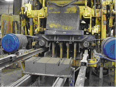
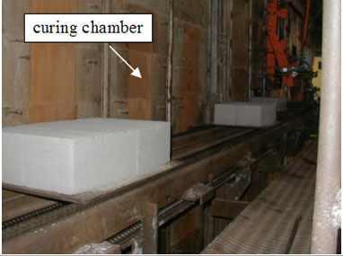
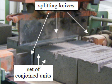
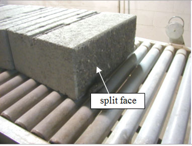
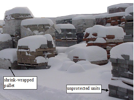
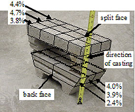
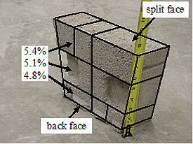
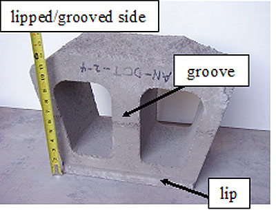
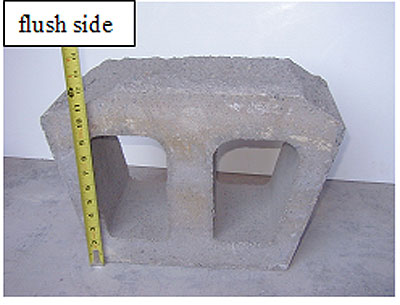
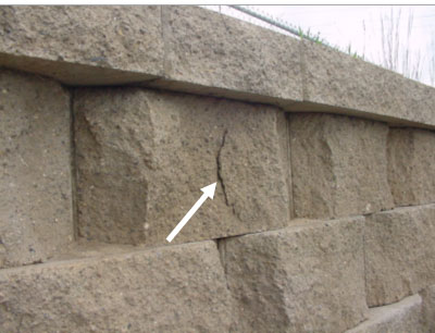
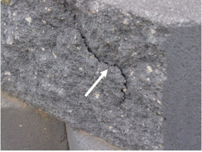
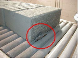
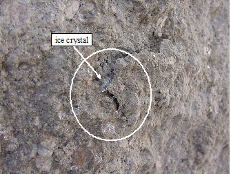
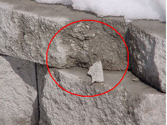
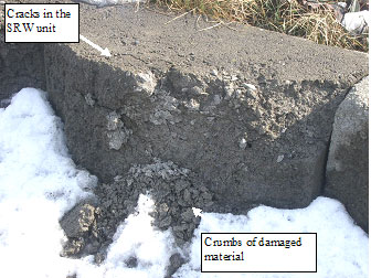
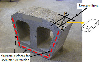
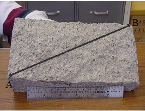
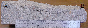
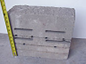
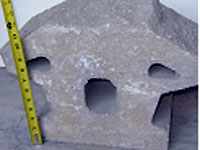
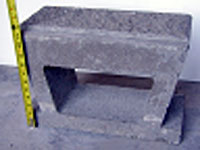
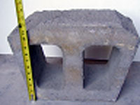
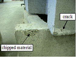
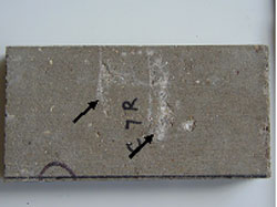
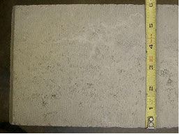
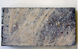
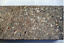
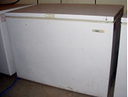
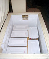
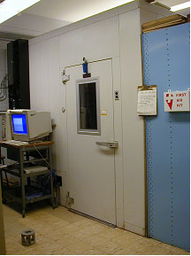
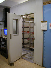
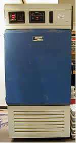
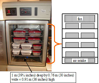
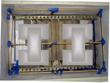
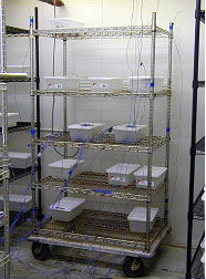
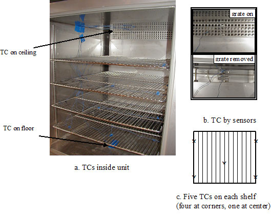
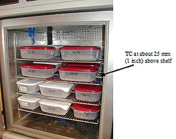
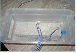
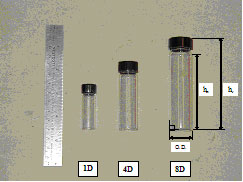
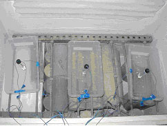
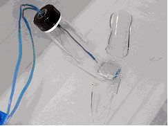
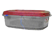
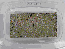

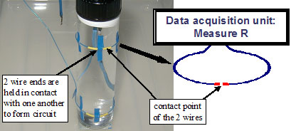
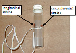
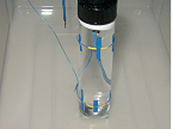
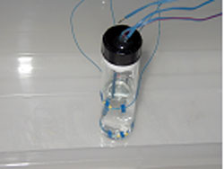

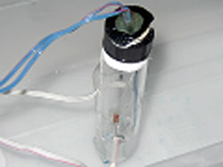
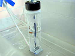
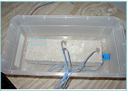
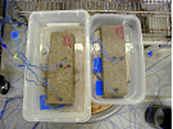
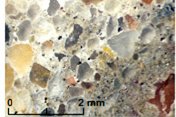
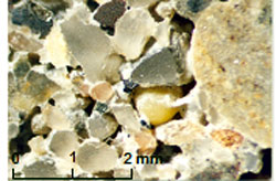
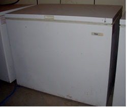
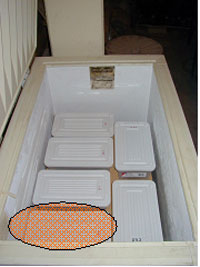

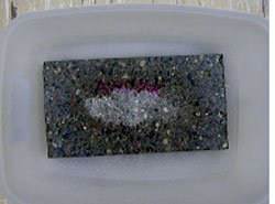
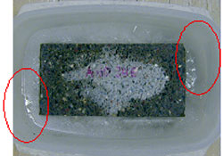
 Equation 9

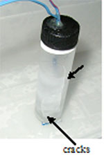
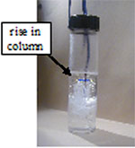
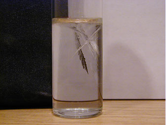
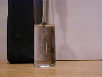
 Equation 10
 Equation 12
 Equation 13