• Federal Highway Administration >
• Publications >
• Research Publications >
• 99194 >
• 07c.Cfm >
• Development and Field Testing of Multiple Deployment Model Pile (MDMP)

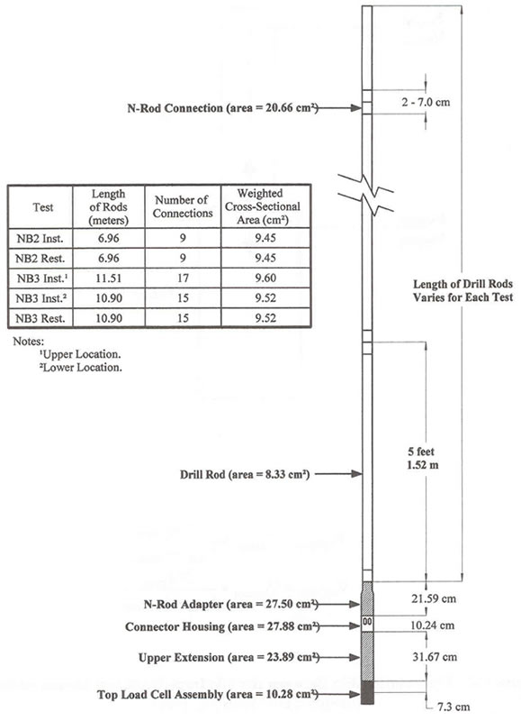
Development and Field Testing of Multiple Deployment Model Pile (MDMP)

CHAPTER 7. ANALYSIS OF THE MDMP TEST RESULTS

7.10 Dynamic Measurements Interpretation

7.10.1 Measured Signals and Wave Mechanics

Section 6.6 presents the dynamic measurements during the various stages of testing. The wave shapes are discussed in great detail, pointing out the variation between the behavior of a homogeneous uniform pile to that of a non-uniform pile. The present section provides the analysis that explains these measurements, in particular, the fact that the lower load cells measured dynamic forces higher than the surface load cells.

Figure 103 presents the make-up of the MDMP segments during the driving of tests NB2 and NB3. As all segments were made of steel, it was assumed that no variation in the modulus of elasticity existed between one segment and the other. As such, the relative variations in the impedance could be taken as the relative variations in the cross-sections. Two distinctive cross-sectional zones existed along the pile - one made mostly of the drilling rods and the other from the rods/MDMP connection to the upper point of measurement inside the MDMP. Table 38 summarizes the weighted areas of each of the sections for the two tests.

Table 38. Variations in the Cross-Section / Impedance Between the Drilling Rods and the MDMP.

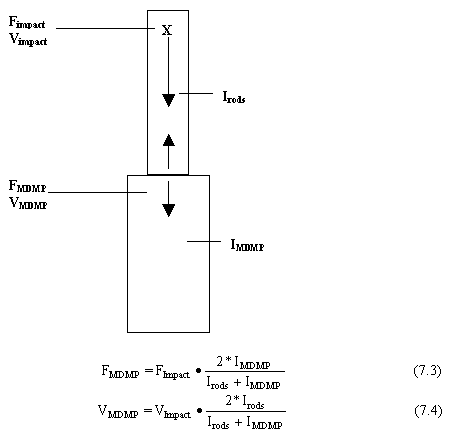
Figure 104 presents a simplified view of the model pile make-up during driving and the influence of the variation in impedance on the traveling force and velocity waves.

Figure 103. Details of the Various Segments That Made Up the MDMP (from the point of surface measurements to the upper inner load cell.

Figure 104. The Relationship Between the Pile Impdedance and Measured Signals (modified after Rausche, 1981).

Substituting the weighted axial cross-sections of Table 38 in equations 7.3 and 7.4 yield the following:

The above ratios can be compared to the values provided in sections 6.6.6 and 6.6.7 for force and velocity measurements, respectively. Using the average measured values presented in Table 28, the ratios of F_MDMP to F_impact were 1.26 and 1.38 for NB2 and 1.25 and 1.34 for NB3 (installation and restrike, respectively). These values matched the simplified calculated ratio of equation 7.5 relatively well and explained the higher impact forces measured inside the pile compared to those measured at the top of the rods. Using the average measured values presented in Table 29, the ratio of V_MDMP to V_impact was 0.75 for NB2 during installation. Again, this ratio compared reasonably well with the simplified ratio obtained from equation 7.6.

The measurements obtained by the internal load cells allowed the assessment of the resisting dynamic forces that acted on the pile during driving. Assuming the frictional force to be concentrated and plastic in nature (activated at once as a response to the motion), the following relationship was valid:

Force_top - Force_middle = 0.5 Resisting Force (7.7)

Where Force_top and Force_middle refer to the measured forces above and below the friction sleeve, respectively. The resisting force on the friction sleeve was, therefore, twice the difference between the simultaneously measured forces at both ends of the friction sleeve. As the force provided in Table 28 reflected the maximum forces, they were not the simultaneously measured forces, but they correctly indicated the magnitudes. Using the values from Table 28 suggested that the dynamic resistance forces along the sleeve varied from about 38 kN during installation to about 52 kN during restrike. These forces were substantially higher than the maximum static forces measured along the friction sleeve (approximately 5.3 kN) and indicated the influence of the dynamic resisting force due to the high-velocity penetration taking place during driving.

7.10.2 Capacity Based on the Energy Approach

The pile capacity was determined using the Energy Approach method (Paikowsky et al., 1994). This simplified method was proven to provide accurate long-term pile capacity based on the dynamic measurements taken during installation. This method utilized the energy delivered to the pile (E) and the maximum displacement (Dmax) as determined from the PDA readings, along with the permanent displacement or set (S) as determined from the driving record (blow count). The calculated resistance was:

The evaluation of MDMP capacity using equation 7.8 is presented in Table 39. The parameters used for the end of driving capacities for NB2 reflected average values for the last 305 mm (12 in) of driving. For the end of the driving capacity of NB3, the first 30 blows were averaged together because the blow count remained constant throughout the installation. The parameters used for the restrike capacities reflected average values for the first five blows.

Table 39. Energy Approach Capacity Predictions for the MDMP.

A comparison between the Energy Approach and the Case method capacities is presented in section 7.10.4 (Figures 117 through 125) in which the variation of the capacity with depth is presented as well.

7.10.3 Capacity Based on CAPWAP Analysis

(1) General.

CAPWAP (Case Pile Wave Analysis Program) (CAPWAP Manual, 1996) solved the wave equation through an iterative process and prescribed measured boundary conditions (e.g., velocity at the top). By varying the resisting forces acting on the pile, a match was obtained between a calculated and a measured additional boundary condition (e.g., force at the top). The static component of the resistance that provided the satisfactory match was assumed to be the static bearing capacity of the pile.

An accurate modeling of the pile was required for the CAPWAP analysis. Since the model pile included a slip joint that was free to open up a space of up to 5 cm (2 in), the modeled pile length depended on the status of the slip joint (open or closed) and the nature of the traveling wave (compression or tension). At any point in time, the slip joint could be closed, partially opened, or completely opened. When the slip joint was closed, a compression wave traveling down was able to travel through the joint, but a returning tension wave coming from the pile tip would be able to travel through the joint as long as the resistance to the slip joint motion was equal to or higher than the magnitude of the traveling wave. In reality, the slip joint would continuously be opening and closing, depending on the magnitude of the traveling waves and the final condition of the slip joint between one impact and the next.

Additional difficulty associated with the CAPWAP modeling of the MDMP was due to the multiple units comprising the MDMP. The one-dimensional wave equation formulation was based on a uniform slender body. Multiple variations in the cross-section had two effects: (1) they created multiple reflections and (2) if the connections between the units were not completely tight, the wave speed was reduced.

During a calibration test for which all the connections were tight, a wave speed of 4,954 m/s (16,254 ft/s) was measured. Small strain reflection tests using a Pile Integrity Tester (PIT) device (PIT Manual, 1993) have resulted in an average wave speed of 5,016 m/s (16,458 ft/s) through one connection. Wave speeds as low as 4,246 m/s (13,931 ft/s) were measured through a connection not properly tightened. These measured velocities were lower compared to the typical wave speed traveling through steel of 5,124 m/s (16,810 ft/s).

All of the above creates major difficulties when modeling the MDMP. Therefore, the CAPWAP analyses were focused on: (1) the restrike data - as CAPWAP results tended to reflect the resistance at the time of measurement, analysis of the records at the beginning of the restrike would potentially be able to determine the long-term capacity; (2) using small-sized pile elements when discretizing the MDMP - such modeling enabled better accommodation for section variability; and (3) examining different combinations when modeling the possible slack at the slip joint (Table 40 presents the cross-sectional areas and the associated lengths used when modeling the MDMP in the CAPWAP analyses).

Table 40. Cross-Sectional Areas for CAPWAP Modeling of the MDMP.

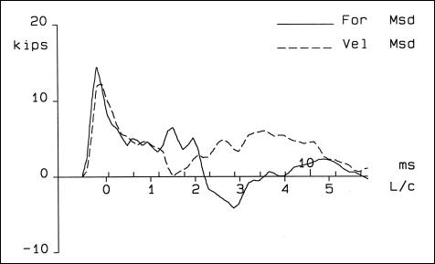
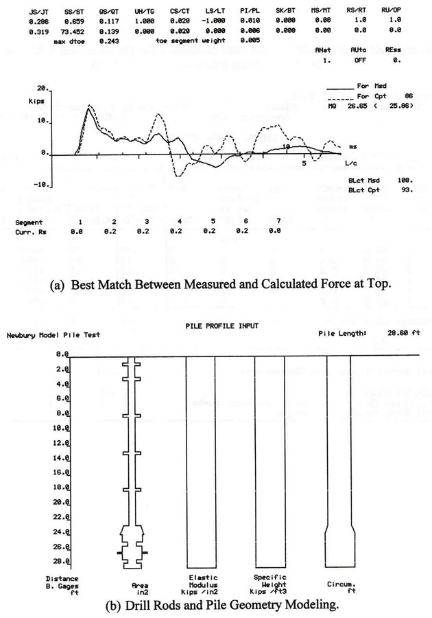
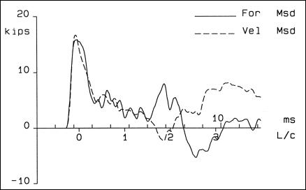
(2) Model Pile Test NB2.

Figure 105 presents the force and velocity (multiplied by the impedance and presented in force units) records for blow 1 of the restrike. Three CAPWAP analyses were performed for this case:

(1) Pile length of 9.88 m (32.4 ft) as a continuous pile.

(2) Pile length of 9.88 m (32.4 ft) with a compression slack of 0.381 mm (0.015 in), 25% effectiveness and a 50.8-mm (2-in) tension slack.

(3) Pile length of 8.72 m (28.6 ft) assuming that the slip joint was practically the end of the pile.

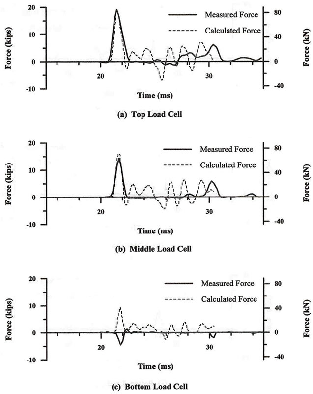
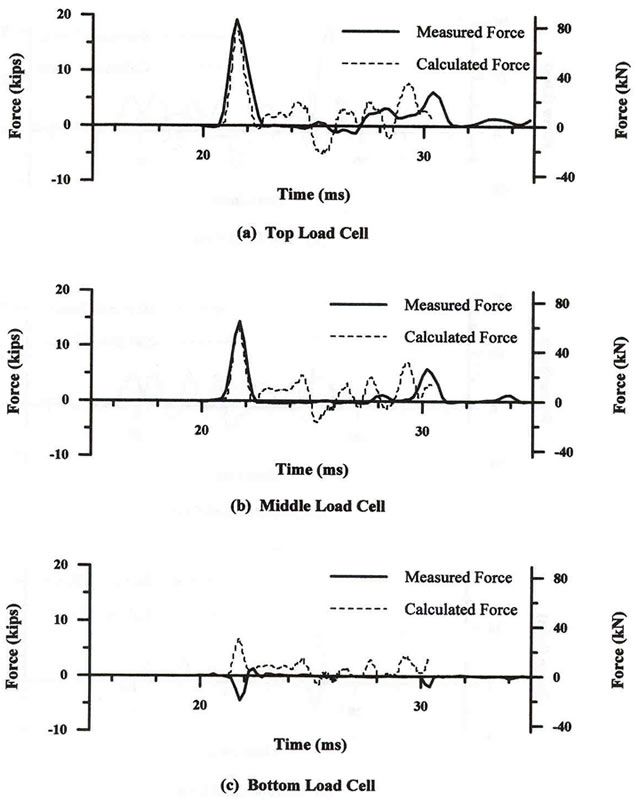
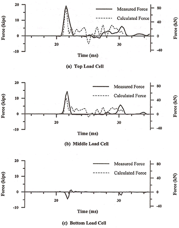
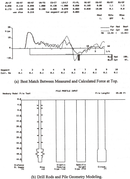
Figure 105. Surface Force and Velocity Records of the MDMP Test NB2 Restrike, Blow 1.

Figures 106, through 108 present the drill rods and pile geometry modeling, along with the associated best match between the calculated and measured forces for the above cases (1), (2), and (3), respectively. Tables 41 through 43 detail the input and output parameters associated with Figures 106, through 108, respectively. A wave speed of 4,938 m/s (16,200 ft/s) was used in these analyses based on a trial-and-error process for the best match over a time period of approximately 1.5 L/c (length/wave speed) (before the embedded section reflection arrived at the top measurement point). Segments of about 15.24 cm (6 in) long were used in all three analyses. CAPWAP analysis of case (1) (refer to Figure 106 and Table 41) resulted in a capacity of 5.3 kN (1.2 kips) with practically no tip resistance. CAPWAP analysis of case (2) (refer to Figure 107 and Table 42) resulted in a capacity of 9.3 kN (2.1 kips), including a 1.3-kN (0.3-kip) tip resistance. CAPWAP analysis of case (3) (refer to Figure 108 and Table 43) resulted in a capacity of 4.4 kN (1.0 kips) with practically no tip resistance.

In spite of the large differences between the modeling conditions and the obtained capacities, similar wave matches were obtained for all cases. A reasonably good agreement existed between the measured and calculated force waves along a time equivalent to about 1 L/c. Most of this length was associated with the stress wave traveling through the drill rods. A consistently poor match existed between 1.5 L/c and 2 L/c, the range that represented the wave reflections from the pile tip. These results suggested that the complex waves that developed due to the large variation in the cross-sections (when moving from the drilling rod to the pile) were difficult to model.

Figure 106. Test NB2 Restrike CAPWAP Modeling of MDMP Case (1): (a) Best Match Between Measured and Calculated Force at Top and (b) Drill Rods and Pile Geometry Modeling.

Table 41. CAPWAP Results of Test NB2 Restrike, Case (1), Assuming a 9.88-m (32.4-ft) Model Pile Without a Slip Joint.

CAPWAP FINAL RESULTS

Total CAPWAP Capacity: 1.2; along Shaft 1.2; at Toe .0 kips

Figure 107. CAPWAP Results of test NB2 Restrike, Case (1), Assuming a 9.88-m (32.4-ft) Model Pile Without a Slip Joint.

Table 42. CAPWAP Results of Test NB2 Restrike, Case (2), Assuming a 9.88-m (32.4-ft) Model Pile With Slip Joint Modeling.

CAPWAP FINAL RESULTS

Total CAPWAP Capacity: 2.1; along Shaft 1.8; at Toe .3 kips

Figure 108. Test NB2 Restrike CAPWAP Modeling of MDMP Case (2): (a) Best Match Between Measured and Calculated Force at Top and (b) Drill Rods and Pile Geometry Modeling.

Table 43. CAPWAP Results of Test NB2 Restrike, Case (3), Assuming a 8.72-m (28.6-ft) Model Pile With Pile Ending at Slip Joint.

CAPWAP FINAL RESULTS

Total CAPWAP Capacity: 1.0; along Shaft 1.0; at Toe .0 kips

Figure 109. Modeling of Case (1), Calculated and Measured Forces at the Internal Load Cell Locations for the MDMP Test NB2 Restrike Blow 1 (analysis based on a force match at the surface measurement location only).

Figure 110. Modeling of Case (2), Calculated and Measured Forces at the Internal Load Cell Locations for the MDMP Test NB2 Restrike Blow 1 (analysis based on a force match at the surface measurement location only).

Figure 111. Modeling of Case (2), Calculated and Measured Forces at the Internal Load Cell Locations for the MDMP Test NB2 Restrike Blow 1 (analysis based on a force match at the surface measurement location only).

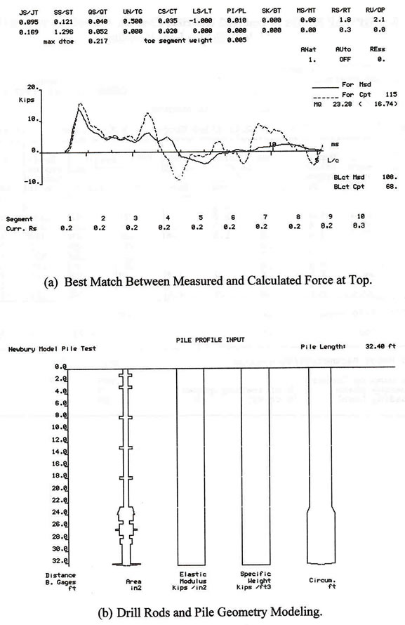
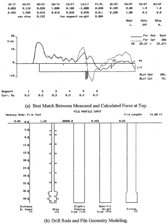
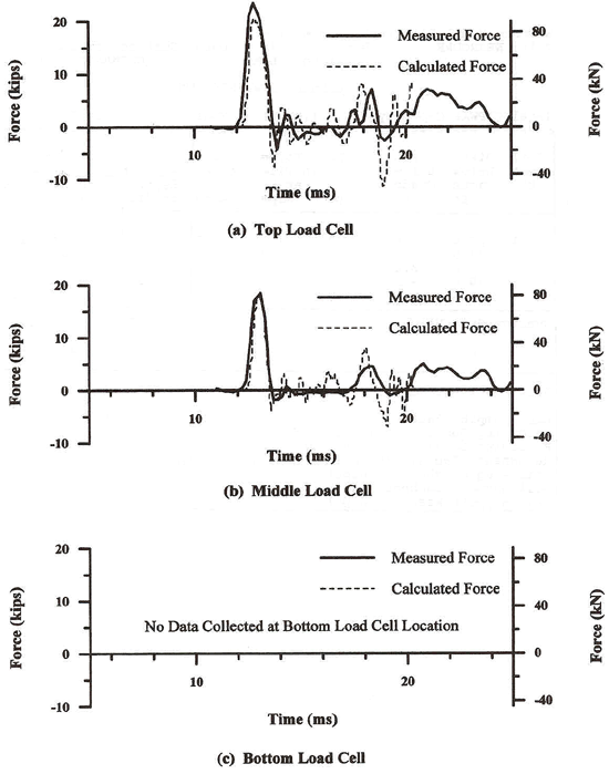
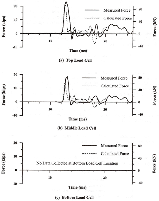
In order to assess the "proper" modeling, the calculated force and measured force (previously presented in Figures 75c and d) associated with the top, middle, and bottom load cells of the three analyzed CAPWAP cases are presented in Figures 109 through 111. The internal measurements were compared to the modeled analyses only upon completion of the top matching process and, hence, did not affect the traditional CAPWAP matching process. Figures 109 through 111 suggest that cases (1) and (2) (for which the full MDMP length was modeled) resulted in a very good match between the measured and calculated traveling wave along the pile. The good match was presented in both magnitude and time for both cases, which means that a full pile length modeling was required and the existence of a slip joint under the compressive wave had not affected the modeled behavior since both cases were similar. The less desirable match obtained for case (3) implied that the assumption of a "short" pile (ending at the slip joint) was not valid. A poor match existed for all cases at the time beyond the major traveling wave. This could be a result of four major factors:

(1) The measurements of small dynamic forces with the large internal load cells were limited in their response and accuracy. The measured forces may have reflected this condition and, hence, did not show the smaller peaks.

(2) A larger damping was required in the CAPWAP modeling of the soil. Such an increased damping coefficient would result in a "smoother" wave shape.

(3) The modeled segment, although it was very short, it was larger than the one required to model accurately the measured motion.

(4) The adopted modeling of the slip joint (case 2) did not correctly reflect the actual physical phenomenon and, hence, did not result in zones of no loading as indicated by the measured records.

(3) Model Pile Test NB3.

Figure 112 presents the force and velocity records for blow 2 of the restrike. Two CAPWAP analyses were performed for this case:

(1) Pile length of 13.84 m (45.4 ft) with a 50.8-mm (2-in) tension slack.

(2) Pile length of 12.68 m (41.6 ft), assuming the slip joint is practically the end of the pile.

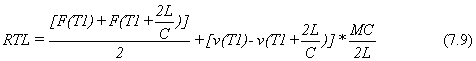
Figure 112. Surface Force and Velocity Records for MDMP Test NB3 Restrike, Blow 2.

Figures 113 and 114 present the drill rods and pile geometry modeling, along with the associated best match between the calculated and measured forces for the above cases (1) and (2), respectively. Tables 44 and 45 detail the input and output parameters associated with Figures 113 and 114, respectively. A wave speed of 4,758 m/s (15,610 ft/s) was used in these analyses, based on a trial-and-error process for the best match over a time period of approximately 1.5 L/c (before the embedded section reflection arrived at the top measurement point). Segments of about 10.16 cm (4 in) long were used in all three analyses. The CAPWAP analysis of case (1) (refer to Figure 113 and Table 44) resulted in a capacity of 5.3 kN (1.2 kips), including a 0.4-kN (0.1-kip) tip resistance. The CAPWAP analysis of case (2) (refer to Figure 114 and Table 45) resulted in a capacity of 8.0 kN (1.8 kips), including a 1.3-kN (0.3-kip) tip resistance.

In order to assess the "proper" modeling, the calculated force and measured force (previously presented in Figures 79c and d) associated with the top and middle load cells of the two analyzed cases are presented in Figures 115 and 116. The internal measurements were compared to the modeled analyses only upon completion of the top matching process and thus did not influence the CAPWAP matching process that was conducted for the measurements at the top of the drilling rods (surface). Figures 115 and 116 reinforce the conclusions previously presented in the analyses of test NB2, restrike blow 1. In summary, the modeling that included the entire pile length provided a good prediction of the stress wave in the pile based on the measurements at the top. However, a variation between the measured and calculated forces beyond the major traveling wave remained questionable and the aforementioned possibilities (see section 7.10.3 part (2) discussion for the NB2 CAPWAP results) remained valid.

7.10.4 Capacity Based on the Case Method

(1) General.

The Case method (see Goble et al., 1970 and Rausche et al., 1972) is a simple field procedure used by the PDA to estimate pile capacities (for a complete review, see Paikowsky et al., 1994). Analysis by the Case method is based on the assumption of a uniform elastic pile, ideal plastic soil behavior, and a simplified wave propagation formulation. Force and velocity measurements taken at the pile top and a correlation between the soil at the pile's tip and a damping parameter are used.

(2) The Case Method Equation.

The Case method calculates the total soil resistance (RTL) activated during pile driving, using the following equation:

where: F(T1) = measured force at the time T1

F(T1+2L/C) = measured force at the time T1 plus 2L/C

v(T1) = measured velocity at the time T1

v(T1+2L/C) = measured velocity at the time T1 plus 2L/C

L, M = length and mass of the pile, respectively

C = speed of wave propagation in the pile.

Figure 113. Test NB3 Restrike CAPWAP Modeling of MDMP Case (1): (a) Best Match Between Measured and Calculated Force at Top and (b) Drill Rods and Pile Geometry Modeling.

Table 44. CAPWAP Results of Test NB3 Restrike, Case (1), Assuming a 13.84-m (45.4-ft) Model Pile With Slip Joint Modeling.

CAPWAP FINAL RESULTS

Total CAPWAP Capacity: 1.2; along Shaft 1.1; at Toe .1 kips

Figure 114. Test NB3 Restrike CAPWAP Modeling of MDMP Case (2): (a) Best Match Between Measured and Calculated Force at Top and (b) Drill Rods and Pile Geometry Modeling.

Table 45. CAPWAP Results of Test NB3 Restrike, Case (2), Assuming a 12.68-m (41.6-ft) Model Pile With Pile Ending at the Slip Joint.

CAPWAP FINAL RESULTS

Total CAPWAP Capacity: 1.8; along Shaft 1.5; at Toe .3 kips

Figure 115. Modeling of Case (1), Calculated and MEasured Forces at the Internal Load Cell Locations for the MDMP Test NB3 Restrike Blow 2 (analysis based on a force match at the surface measurement location only).

Figure 116. Modeling of Case (2), Calculated and Measured Forces at the Internal Load Cell Locations for the MDMP Test NB3 Restrike Blow 2 (analysis based on a force match at the surface measurement location only).

Different variations of the Case method have been developed taking T1 as the time of impact or modified to include a time delay constant allowing higher RTL values to be obtained. The time T1 is defined, in equation form, as:

where: TP = time of the impact peak

d = time delay.

In most cases, d = 0. However, the time delay is required in soils capable of large deformations before achieving full resistance. A time delay is also used in situations where the hammer impact is uneven (PDA Manual, 1996). Several factors that influence the pile-soil system must be considered when the total predicted resistance is evaluated. These factors include time-dependent soil strength changes and refusal driving when the soil's resistance is not fully mobilized under a single hammer blow.

The total resistance calculated is a combination of the static resistance (S), which is displacement dependent, and the dynamic resistance (D), which is velocity dependent. Therefore, the total resistance (Goble et al., 1975) is:

The dynamic resistance D is considered to be viscous in nature, hence, it is a function of the velocity at the pile toe (V_toe) and a damping constant (J) where:

        (7.12)

By applying the wave propagation theory, the pile toe velocity can be calculated as a function of the velocity at the pile top:

where: L = pile length

M = pile mass

C = wave speed of the pile material

RTL = total resistance

V_top = velocity at pile top.

V_top is taken as the pile top velocity at the time T1.

According to Goble et al. (1975), remolding effects cause the majority of the damping resistance to be concentrated near the pile tip. Consequently, the damping constant is determined according to the soil type at the pile tip. In most cases, the damping constant (J) is proportional to the pile properties (EA/C), and is, therefore, represented by a dimensionless coefficient (J_c) using the following equation:

where: J_c = dimensionless Case damping coefficient

E = elastic modulus of the pile material

A = pile cross-sectional area

C = wave speed of the pile material.

Recommended J_c values are provided according to soil type (PDA Manual, 1996). These values keep changing over the years as a result of improvements to the PDA and continued research in this area. Paikowsky and Chernauskas (1996) had clearly demonstrated that the use of viscous damping parameters for pile-penetration modeling was in lieu of soil inertia that was not accounted for in the pile-penetration formulation. As such, Paikowsky and Chernauskas have shown a better correlation between viscous damping parameters and the combination of pile size and blow count rather than soil type.

(3) The Maximum Resistance Method (RMX).

Several variations of the Case method have evolved for the analysis of different driving situations and soil types. The variations are similar in that they all begin with the initial total resistance prediction (RTL) of equation (7.9). Five distinct methods employ the predicted RTL: the Damping Factor Method, the Maximum Resistance Method, the Minimum Resistance Method, the Unloading Method, and the Automatic Method. A brief review of the method most commonly used (the Maximum Resistance Method) follows. By substituting equation (7.13) into equation (7.12), and this, in turn, into equation (7.11) (expressed as the static pile resistance component, RSP), one obtains the standard Case Method equation:

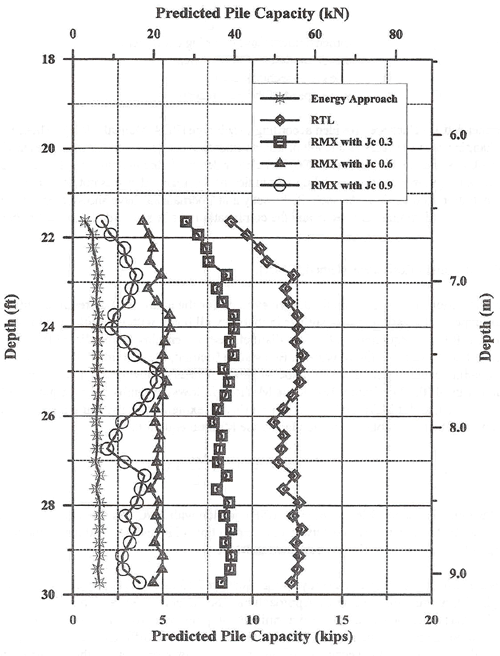
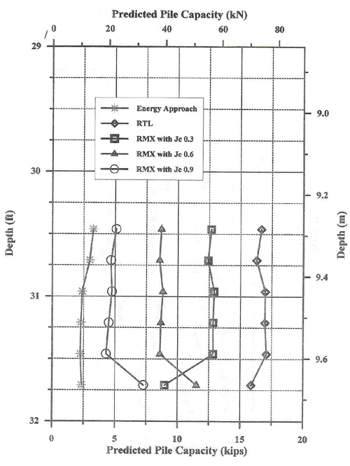
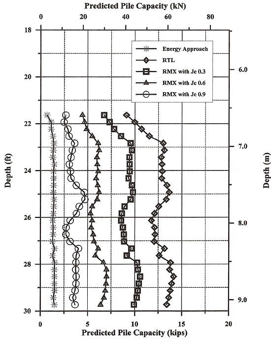
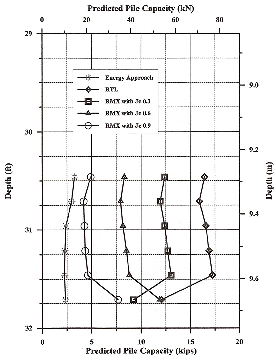
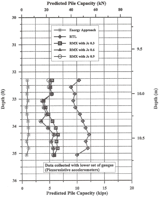
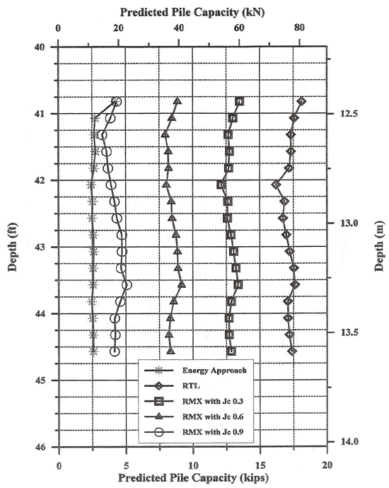
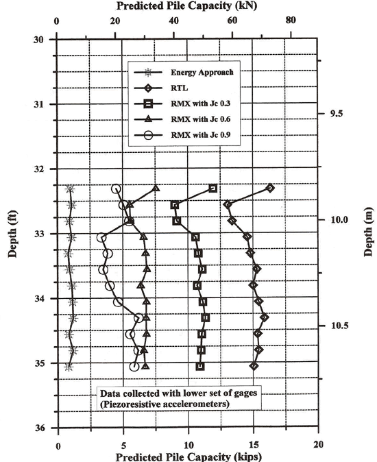
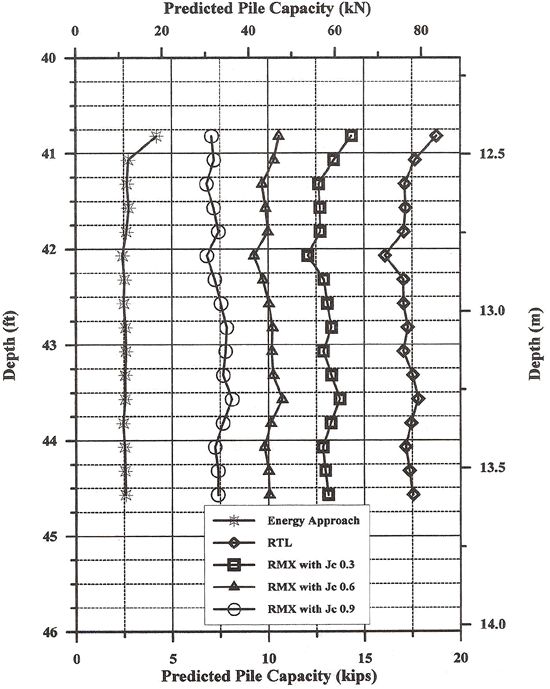
The Maximum Resistance Method uses the RSP equation with 2L/C as a fixed quantity. The time T1 used in the RSP equation is varied between the impact time (TP) and TP + 30 ms to find the corresponding maximum RSP value, denoted as RMX.

The evaluation of the MDMP capacity using equation 7.15 as RMX is presented in Figures 117 through 124, along with the Energy Approach method capacity (see section 7.10.2 and equation 7.8). The Case method capacity was determined using the pile properties of the drill rods and was based on the measurements obtained at the surface. Three different damping factors were examined, investigating the sensitivity of the calculated static capacity to the variations in the damping coefficient. Figures 117 and 118 present the capacity determined for the MDMP test NB2 installation and restrike data, assuming the wave reflection from the pile tip (pile length was 9.88 m) as in cases (1) and (2). Figures 119 and 120 present the capacity determined for MDMP test NB2 for installation and restrike data, assuming that the wave reflection was related to the slip joint (pile length was 8.72 m) as in case (3). Figures 121 and 122 present the capacity determined for MDMP test NB2 for installation and restrike data, assuming the wave reflection from the pile tip (pile length was 13.84 m) as in case (1). Figures 123 and 124 present the capacity determined for MDMP test NB2 for installation and restrike data, assuming that the wave reflection was related to the slip joint (pile length was 12.68 m) as in case (2).

Figure 117. Predicted Pile Capacity for the Installation of MDMP Test NB2 (Cases 1 and 2) Based on the Energy Approach Method and the Case Method With Varying Jc Values (assuming pile length is 9.88 m (32.4 ft)).

Figure 118. Predicted Pile Capacity for the Restrike of MDMP Test NB2 (Cases 1 and 2) Based on the Energy Approach Method and the Case Method With Varying Jc Values (assuming pile length is 9.88 m (32.4 ft)).

Figure 119. Predicted Pile Capacity for the Installation of MDMP Test NB2 (Case 3) Based on the Energy Approach Method and the Case Method With Varying Jc Values (assuming pile length is 8.72 m (28.6 ft)).

Figure 120. Predicted Pile Capacity for the Restrike of MDMP Test NB2 (Case 3) Based on the Energy Approach Method and the Case Method With Varying Jc Values (assuming pile length is 8.72 m (28.6 ft)).

Figure 121. Predicted Pile Capacity for the Installation of MDMP Test NB3 (Case 1) Based on the Energy Approach Method and the Case Method With Varying Jc Values (assuming pile length is 13.84 m (45.4 ft)).

Figure 122. Predicted Pile Capacity for the Restrike of MDMP Test NB3 (Case 1) Based on the Energy Approach Method and the Case Method With Varying Jc Values (assuming pile length is 13.84 m (45.4 ft)).

Figure 123. Predicted Pile Capacity for the Installation of MDMP Test NB3 (Case 2) Based on the Energy Approach Method and the Case Method With Varying Jc Values (assuming pile length is 12.68 m (41.6 ft)).

Figure 124. Predicted Pile Capacity for the Restrike of MDMP Test NB3 (Case 1) Based on the Energy Approach Method and the Case Method With Varying Jc Values (assuming pile length is 12.68 m (41.6 ft)).

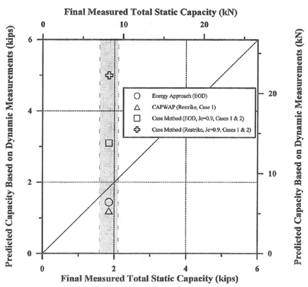
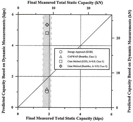
All analyses consistently presented the Energy Approach predictions as being the lowest, whereas the total resistance (RTL) of the Case method was roughly 5 to 10 times the values predicted by the Energy Approach. Since the Energy Approach was based on a simplified elasto-plastic soil resistance relationship without referring to dynamic losses, it consistently presented higher resistance values. The fact that the Case method's various calculations were so much higher suggested that the different values of force and velocity used in its evaluation (in particular, those related to the time T1+2L/C, see equation (7.9)) were strongly affected by the MDMP geometry and, hence, not applicable to the Case method formulation. The high velocities measured during driving explained the large variations in the static resistance values when changing the damping coefficients. The small variation of resistance with depth reasonably reflected the small variation in resistance expected to take place in a clay layer over a small penetration depth. This is in sharp contrast to the variations that existed between the methods, or the variations that existed as a result of the changes in the damping coefficient.

7.11 Comparison Between the Static Capacity and the Analyses Based on Dynamic Measurements

The complexity of the MDMP testing in regards to time and methods resulted in a variety of static resistances, which raised difficulties for obtaining a single representative value. Table 46 summarizes the different resistances encountered during the final pull-out and compression tests. The discrepancy between the sleeve frictional resistances during pull-out and compression tests were discussed earlier (see section 7.8). A reasonable assessment was provided based on the surface load cell readings during the final compression tests of MDMP tests NB2 and NB3 for 7.15 kN (1.61 kips) and 7.01 kN (1.58 kips), respectively. Using an average of 7.09 kN (1.59 kips) provided a lower estimation for the total capacity. A higher end estimation of the static capacity could be obtained from the surface load cell measurements in the final pull-out tests for 9.91 kN (2.23 kips) and 8.85 kN (1.99 kips) for MDMP tests NB2 and NB3, respectively. Using an average of these values, 9.36 kN (2.11 kips) provided a higher estimation of the total capacity. A reasonable range for the MDMP static capacity for both tests was, therefore, 7.09 kN (1.59 kips) to 9.36 kN (2.11 kips).

The above range was compared to the prediction of the various dynamic analyses in Figures 125 and 126 for MDMP tests NB2 and NB3, respectively. The following methods and conditions were chosen for the dynamic analyses:

(1) Energy Approach Method for end of driving records (EOD). As the Energy Approach method was developed for the driving condition, its use for restrike measurements was not recommended.

(2) CAPWAP analysis results for restrike measurements using the full-length pile modeling (case 1).

(3) Case method (RMX) value using a high damping factor of J_c = 0.9 and records from EOD and restrike.

Table 46. Summary of the MDMP Final Static Capacities During the Tension (Pull-Out) and Compression Load Tests.

Figure 125. Comparison Between the Measured Static Capacity for MDMP Test NB2 and Predictions Based on the Dynamic Measurements Utilizing Various Methods of Analysis.

Figure 126. Comparison Between the Measured Static Capacity for MDMP Test NB3 and Predictions Based on the Dynamic Measurements Utilizing Various Methods of Analysis.

The obtained results suggested that the Energy Approach method for the EOD records and CAPWAP for the restrike records provided the best predictions for the long-term measured capacities. Both methods underpredicted the measured capacities by approximately 29% and 40% for NB2 and NB3, respectively (referring to the average of the static capacity zone). The Case method predictions for both EOD and restrike were substantially higher than the measured capacity. This observation was most likely associated with the incompatibility of the method with the make-up of the MDMP due to its influence on the values used in the Case method analysis.