• Federal Highway Administration >
• Publications >
• Research Publications >
• 02110 >
• Nondestructive Evaluation >
• Support of The System Test and Analysis Program for The Nationwide Differential Global Positioning System Modernization Program

Support of The System Test and Analysis Program for The Nationwide Differential Global Positioning System Modernization Program

FHWA Contact: Jim Arnold, HRDI-06,
202-493-3265, james.a.arnold@dot.gov

The Nationwide Differential Global Positioning System (NDGPS) Modernization Program is a multiagency effort to examine the viability of long baseline carrier phase differential correction techniques. Phase I of this program analyzes broadcasting Global Positioning System observables from a single NDGPS site, Hagerstown, MD, to aid in determining the appropriate signal structure and compression techniques to support long range carrier phase operations. Phase II will install a second facility near Hawk Run, PA, enabling multiple baseline carrier and code phase navigation solutions.

This first report verifies that the accuracy that can be achieved over a long baseline from a single facility is within the estimated 10-centimeter (95 percent) horizontal navigation accuracy hypothesized.

NOTICE

This document is disseminated under the sponsorship of the U.S. Department of Transportation in the interest of information exchange. The U.S. Government assumes no liability for its contents or use thereof. This report does not constitute a standard, specification, or regulation.

The U.S. Government does not endorse products or manufacturers. Trade and manufacturers' names appear in this report only because they are considered essential to the object of this document.

Table of Contents

1. Introduction
1.1 Background
1.2 The Current NDGPS System
1.3 RTCM-104 Correctors (A Public Broadcast Format Example)
1.4 Added RTCM-104 Messages to Support Centimeter Applications
1.5 Message Size
1.6 Organization

2. System Architecture

3. Functional Components
3.1 GRIM: A Brief Overview
3.2 Hydra and DynaPos

4. Compression and Data Categories
4.1 Bandwidth and Frequency
4.2 Base Station Data (from Hagerstown, MD)

5. Data Results
5.1 General Remarks
5.2 Raw Carrier Measurements Versus Carrier Measurements Received by User
5.3 Raw Code Measurements Versus Code Measurements Received by User
5.4 Brief Remarks Regarding the Number of Missed Data Packets

6. Static and Dynamic Applications (46 km and 250 km)
6.1 Static Examples (Hydra)
6.2 Dynamic Example (Dynapos)

7. Conclusions

Appendix A-Phase I Participation Options

Appendix B- Support of the System Test and Analysis Program for the NDGPS Modernization Program

List of Figures

Figure 1. Hagerstown— The HA-NDGPS Broadcast Station Rack
Figure 2. The Hagerstown GRIM Software Display
Figure 3. The Hagerstown Ashtech and Trimble Antennas
Figure 4. L1 Carrier Data: Raw Versus User-Received Compressed and Decompressed
Figure 5. L2 Carrier Data: Raw Versus User-Received Compressed and Decompressed
Figure 6. L1 Code Data: Raw Versus User-Received Compressed and Decompressed
Figure 7. L2 Code Data: Raw Versus User-Received Compressed and Decompressed
Figure 8. Number of Lost Packets During Chesapeake Bay Tests
Figure 9. Real-Time Hydra Plot Done at Facility near Dickerson, MD
Figure 10. Real-Time Static Plot Performed near Dickerson, MD
Figure 11. Real-Time Versus Post-Processed Ellipsoidal Height
Figure 12. Real-Time Navigation Solution Compared to Post-Processed Solution
Figure 13. Dynamic Results on a Stationary Platform
Figure 14. Error Due to Data Compression
Figure 15. Effects of Missing Epochs

1. Introduction

1.1 Background
When the Department of Defense (DoD) originally developed the Global Positioning System (GPS), it was a military system. GPS quickly became a tool for both military and civilian applications across the world. Initially, DoD intentionally degraded GPS signals. To compensate, civilian and military engineers placed equipment at specific sites to determine intentional errors. These errors were then broadcast to users who would correct their measurements. Because these corrections did not compromise security, Differential GPS (DGPS), as these corrections came to be known, flourished with little opposition from DoD. Because DGPS delivered nominally 6- to 20-meter (m) accuracy, the U.S. Coast Guard (USCG) developed a DGPS system along the U.S. coasts and waterways. The success of this system encouraged other governmental agencies to make such capabilities available in other parts of the country, particularly in the West and Midwest. This national extension is known as the Nationwide DGPS (NDGPS). The NDGPS is advertised as a 1-3-m system with 99.97 percent availability. NDGPS can deliver meter-level accuracies. The new vision, High Accuracy-NDGPS (HA-NDGPS), is designed to broadcast additional information from the same NDGPS network using a new carrier frequency to achieve fixed and/or moving centimeter (cm)-decimeter (dm)-level accuracies while maintaining as much integrity as possible. HA-NDGPS, and the ability to implement the system cost-effectively, is the subject of this report.

1.2 The Current NDGPS System
The USCG developed the original DGPS network. The U.S. Army Corps of Engineers (USACOE) needed a similar capability along inland waterways and, with the help of the USCG, established USCG-like broadcast stations. USACOE later adopted the NDGPS concept and developed additional stations. The US Department of Transportation (USDOT) continues to install NDGPS stations at retired Air Force Ground Wave Emergency Network (GWEN) sites. When installation is completed, there will be approximately 137 similar stations broadcasting Course/Acquisition (C/A) code correctors to users. This will enable meter-level positioning with an associated level of integrity.

1.3 RTCM-104 Correctors (A Public Broadcast Format Example)
These beacons today broadcast single-frequency GPS code range correctors enabling few-meter level positioning and navigation along the U.S. coasts and inland waterways. An expected pseudorange value is computed for each GPS satellite in view at the NDGPS sites. These computed values are compared with the actual pseudorange measurements made at the sites; the difference is known as a pseudorange corrector. The assumption is that the errors are common to both the reference site and any user site. These correctors are placed in a formal bit stream with message header, message type, and with parity considerations and broadcast to users as a Type 9 message. This message is one of many broadcast as part of the RTCM-104 protocol developed by the Radio Technical Committee for Maritime Services (RTCM). The work of the RTCM committee is documented amply elsewhere; this report only provides a brief summary.

Based upon the RTCM-104 message, users are able to perform meter-level positioning in static or moving applications. This message requires approximately 660 bits to send C/A code pseudorange correctors for 12 satellites. It should be noted that correctors are sent because correctors are expected to require fewer bits than observations. As a corollary, one can assume that sending complete C/A code pseudoranges (for 12 satellites) would have taken more bits.

1.4 Added RTCM-104 Messages to Support Centimeter Applications
In the early 1990s, there was a need for a standard message that could support accuracies better than what the RTCM-104 provided. The RTCM committee developed two message types—18 and 19, and 20 and 21—to meet that need. Pairs 18 and 19 proved a more practical choice, because both pairs had similar bit sizes, but pairs 18 and 19 provided users a message protocol compatible with decimeter, centimeter, and even subcentimeter positioning. It should be noted that pairs 18 and 19 require approximately 3000 bits to broadcast the full suite of dual code and carrier measurements required by high-precision users.

With this proposed RTCM enhancement, centimeter-level survey and dynamic positioning became possible (i.e., based upon an open format) in support of surveying, transportation, and other industrial uses.

This format, however, is too large to fit within the bandwidth allotted to HA-NDGPS.

1.5 Message Size
There are other formats available for sending code and carrier measurements or correctors over a link to a user. Some of these are proprietary and little is known about them. Other formats are currently under development. As we will discuss later, it is very desirable to fit the entire GPS carrier and code observations for 12 satellites within 800 to 1000 bits per second.

Experience with Medium Frequency Data Links has shown that, time-wise, shorter messages provide substantial performance advantages. In cases in which pseudorange corrections are sent, corrections can be broadcast in messages that contain only subsets of satellites. For carrier phase observables, it may be preferable to package all the observables from a given epoch in a single message. To maximize code and carrier synergy, it also may be desirable to maintain the inclusion of code and carrier observables in a single message.

The Federal Highway Administration (FHWA) converted GPS dual-frequency code and carrier measurements at Hagerstown, MD, into a message stream that was sent to a modulator. FHWA then interfaced the modulator output to the HA-NDGPS transmitter, the output of which was combined (i.e., diplexed) with the current NDGPS broadcast signal for final broadcast over the air to the equipped user. It was necessary to fit the GPS measurements or correctors (12 satellites) within approximately 1000 bits.

FHWA then sent a stream of bits to the Government Furnished Equipment (GFE) demodulator for translation (i.e., decompression) of the message into useable data for resulting measurements and to demonstrate high-precision positioning results. Real-time static survey was demonstrated at 46 kilometers (km) using Hydra& software. Real-time moving application was demonstrated at 250 km using DynaPos& software.

1.6 Organization
This report first describes the overall system architecture.

The report then explains GRIM& (GPS Receiver Interface Module, developed by XYZ GPS Inc.) and its interface with GFE and Hydra and DynaPos application modules for demonstrating accurate static and dynamic positioning.

The next chapter covers compression and data categories, after which data results are presented. Static and moving positioning examples are provided, followed by suggestions for participation in concept validation. The report ends with a summary and conclusions. See workshop proceedings for findings from an April 10, 2002, HA-NDGPS workshop.

2. System Architecture

The Hagerstown DGPS site is located at approximately 39° 33' 11" north and 77° 42' 51" west. A system block diagram can be found in the workshop proceedings from an April 10, 2002, HA-NDGPS workshop.

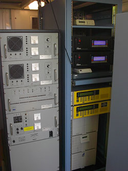
Figure 1. Hagerstown—The HA-NDGPS Broadcast Station Rack

An existing Ashtech Z-12 GPS receiver provides the operational DGPS network. A second output port from the same receiver transmits 1 Hz dual-frequency GPS code and carrier measurements to a PC via an RS-232 port into the GRIM software module.

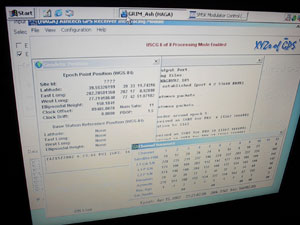
Figure 2. The Hagerstown GRIM Software Display

GRIM plays two important roles. The most important is to compress the data into the allocated bandwidth and pass the resulting "packet" to the GFE modulator. GRIM's other primary role is to log the data in one or more formats: Raw Ashtech Port Output for possible future playback; compressed packets for possible future playback; or RINEX for future processing. During these tests, it has been essential to store the raw data on the Hagerstown site PC, because these data represent the data reference against which all comparisons ultimately are made. The other two data types can be re-created exactly with GRIM in a playback mode. In a fully mature system, it may be satisfactory to save the compressed data, because it requires only 10 percent of the space occupied by raw receiver output data.

GRIM passes the data packets to the GFE modulator, and the GFE modulator readies the packet for transmission.

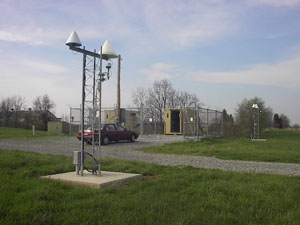
Figure 3. The Hagerstown Ashtech and Trimble Antennas

The Hagerstown transmitter broadcasts the message omnidirectionally over an approximately circular area of radius 225 km or more. As discussed below, a successful moving test was conducted on the Chesapeake Bay roughly 250 km from Hagerstown. At 46 km, for example, there were very few missed data packets (0-10 per day with the current equipment). At 245 km, testers were beyond the recommended range, but even at this distance, there were very few missed data packets away from dockside on the Chesapeake Bay.

A PC is necessary at this early phase in the development cycle. As research progresses, the demodulator and decompression functions likely will be built into the GPS receiver, much like a Wide Area Augmentation System receiver.

3. Functional Components

3.1 GRIM: A Brief Overview
GRIM was developed to convert or translate different GPS receiver hardware to a single interface. GRIM also performs many other functions. GRIM provides data logging services in a variety of formats. The module also can command a GPS receiver into various configurations and provides a suite of data compression choices to fit a variety of data streams and bandwidths. GRIM provides a playback feature that permits a replay of real-time data either to troubleshoot actual real-time situations or to permit post-mission processing. GRIM provides data streams to applications and can provide the same data, simultaneously, to multiple applications or multiple copies of the same application.

Base Station GPS Receiver to GRIM and GRIM to Modulator
In the HA-NDGPS situation, GRIM takes in raw GPS measurements, compresses them, and creates message packets to be passed on to the GFE modulator. There are many possible data packet definitions that could be selected depending on what data types need to be sent and specific bandwidth limitations. Whatever data compression scheme is selected, the data packet header includes the data definition, so that a user would continue to function even if the packet definition should change. This has been described as "self-defining."

Demodulator to GRIM and GRIM to Application
During this Phase I period, GRIM has a second function at the user end. In this case, GRIM receives a bit stream (which is a compressed data packet) from the user site demodulator and decompresses it. Finally, GRIM passes the standardized GRIM output to the user application software.

3.2 Hydra and DynaPos
Hydra is a software application that performs real-time (and playback) static surveying and monitors hazardous motion. For this report, researchers used Hydra in static survey mode 46 km from the Hagerstown site. The goal was to demonstrate that Hydra achieves subcentimeter survey results based upon the HA-NDGPS broadcast. The results are similar to findings with the raw data collected at the site. This demonstrates that the HA-NDGPS broadcast information is nearly identical with post-mission data; therefore, results similar to post-mission results can be expected.

DynaPos is another real-time (and playback) software application for moving applications such as hydrographic surveying, farming, or real-time kinematik (RTK) DynaPos was run on static data that was treated as moving data and consistently achieved steady-state positioning at the half-decimeter level for north and east components and decimeter-level for the height component. Values given are 1-sigma values.

DynaPos later was used in a real-time test running from Tangier Island, VA, to Crisfield, MD, on a mail boat. Actual real-time kinematic positioning results were compared with post-mission results using raw data and with local results from Tangier Island to the mail boat.

Although it is understood that precise carrier phase GPS methods work, researchers were trying to demonstrate that the broadcast data that reaches the user agrees at the millimeter level with the original data. This is proof that the HA-NDGPS broadcasts will support proven high-precision methods, provided the data actually reaches the user intact.

4. Compression and Data Categories

4.1 Bandwidth and Frequency
The ability to squeeze dual- (and even triple-) frequency GPS code and carrier data or correctors into a small bandwidth is important because bandwidth is precious. It also is preferred to deliver the data on a carrier signal of lower frequency. A lower frequency signal becomes necessary to reach well beyond the line of sight. Depending on output power and height of the transmission tower, a transmitter might reach 75 km with a high-frequency line-of-sight signal, but in contrast, the same transmitter could reach 3-4 times that far with a lower frequency signal that can follow the ground and curvature of the earth. The difference between a high-frequency and a low-frequency signal easily can be a 10-fold factor in terms of the number of sites required. There is yet another factor that is critical to robust delivery. Low-frequency signals are more useful in buildings, forests, valleys, etc., than are high-frequency line-of-sight signals.

It is desirable to reduce the current message to 800 or fewer bits in anticipation of the third civilian GPS frequency, and progress with respect to further compression continues to be made.

It should be noted that, while bit size is important, it is not the sole metric for choosing a compact message. For example, data packets must be "self-contained" and "self defining." Other qualities for consideration are flexibility and growth.

4.2 Base Station Data (from Hagerstown, MD)
Three categories of base station data are defined below.

Raw Base Station Data (GPS Receiver Output)
Raw base station data is simply data as it is output from the GPS receiver port. These data are not altered and are saved on the Hagerstown hard drive. For this report, such data represents truth data. The data will be compared with what the user receives over the air from the HA-NDGPS broadcast. It is important to determine how much data does not reach the user (as a function of distance) and how well the data received agrees with this raw truth data (i.e., any differences would be caused by compression).

Compressed Data Ready for Broadcast (None missing yet)
These data are compressed and prepared for the modulator. It is possible to save these compressed data along with the raw data. Since these data require much less hard drive space compared to raw data, it might be preferable to store compressed data instead of raw data, however, the raw data is the most fundamental, of course.

Compressed Data Received by a User (Lost packets are possible as a function of distance or SNR)
The compressed data received by the user can be different from the compressed data that was actually sent in two primary ways. The first possibility is that the signal strength of the broadcast could be very weak, perhaps as a result of the transmitter being too far away. In this case, the data packet might be garbled so that the checksum (actually circular redundancy check) does not agree with the packet. The data must be discarded, as there is no data repair feature. The second possibility is that the user's equipment is not turned on, so no data can be received. This report only determines the percentage of missed packets as a function of distance, at 46 km and at 250 km.

5. Data Results

5.1 General Remarks
At the Dickerson site, REMD, the signal-to-noise ratio (SNR) was approximately 25 decibels (dB), and the signal strength was approximately 67 dBW. During the May 2002, Tangier Island test, at more or less 245 km distant, the SNR was approximately 13-15, and the signal strength was approximately 33. Researchers determined that an SNR of roughly 13 was required for the broadcast data to be demodulated and decompressed. At 46 km, missed packets were rare (possibly 0-10 per day), whereas at 250 km, missed packets were a lot more frequent (perhaps 10 per hour on the Chesapeake Bay and approaching 100 per hour at times at dockside). At 46 km, the signal was sufficiently strong that obstacles did not appear to cause lost packets, but at 250 km, obstacles such as buildings appeared to become a factor. Therefore, there were many missed packets (more than 1 percent) at dockside at Tangier Island, but on the Chesapeake Bay at the same transmission distance, there were relatively few lost packets.

5.2 Raw Carrier Measurements Versus Carrier Measurements Received by User
Below are data comparisons between raw GPS receiver data and the data received over the air at a facility 46 km away. The plots are striped, because the truth data was written to RINEX files having 0.1-millimeter (mm) precision. The worst-case difference between the L1 carrier phase truth data and the user data is 1.41 mm, as expected. The root-mean-square (RMS) difference was smaller than 1 mm. The results were very similar for the L2 carrier data.

It should be noted that in both cases, the differences have a mean of essentially 0.0 and are expected to have no impact on static surveys and a negligible positioning error on moving surveys. In real life, multipath and internal receiver noise are much greater and do not yield a mean zero error over a few seconds.

Figure 4. L1 Carrier Data: Raw Versus User-Received Compressed and Decompressed

Figure 5. L2 Carrier Data: Raw Versus User-Received Compressed and Decompressed

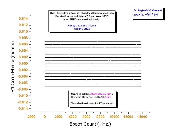
5.3 Raw Code Measurements Versus Code Measurements Received by User
Next are data comparisons between raw GPS receiver code data and the data received over the air at a facility 46 km away. The plots are striped because the truth data was written to RINEX files having 1 mm-precision. The worst-case difference between the L1 code phase truth data and the user data is 7 mm, as expected. The RMS difference was roughly 4 mm. The results were very similar for the L2 code data.

It should be noted that in both cases, the differences have a mean of essentially 0.0 and are expected to have no impact on code-based static or moving applications and no impact on initializing high-precision carrier-phase surveys.

Figure 6. L1 Code Data: Raw Versus User-Received Compressed and Decompressed

Figure 7. L2 Code Data: Raw Versus User-Received Compressed and Decompressed

5.4 Brief Remarks Regarding the Number of Missed Data Packets
At 46 km
As stated elsewhere in this report, there were very few missed packets at the facility located 46 km from Hagerstown. The number of missed packets at this site was too few for plotting purposes. There were many days in which there were no missed packets; on other days there were as many as 10 missed packets.

At 250 km
The following plot indicates the number of missed packets that might be encountered at the limits of the Hagerstown broadcast range. Here the signal is quite weak, and receiving the signal away from obstructions did make quite a difference.

In the field, transmissions received in the middle of the Chesapeake Bay resulted in the fewest number of missed packets. Transmissions to dockside at Tangier Island (where there were buildings and other signal obstructions) resulted in a larger number of missed packets. A combination of atmospheric conditions and obstructions may have been responsible for this contrast. Even then, we were able to continue our real-time application.

Figure 8. Number of Lost Packets During Chesapeake Bay Tests

6. Static and Dynamic Applications (46 km and 250 km)

6.1 Static Examples (Hydra)
Base Data
From April to June 2002, the GFE reception equipment was operated in Dickerson, MD, 45.8 km from the Hagerstown broadcast station. The equipment included a low frequency antenna which picked up the broadcast signal, a demodulator (and its power source) to process those signals, a laptop computer for ingesting demodulated, compressed messages, and GRIM software for decompressing the compressed message into standard output. Normally this GRIM output was saved to the hard drive for later comparisons and playback, and sent to an application program such as Hydra or DynaPos.

User Data
In addition, a GPS receiver took and ingested data into a second GRIM on the same computer that was ingesting the demodulator signal. These user data were saved to the hard drive for playback and sent to Hydra and/or DynaPos.

Hydra (also known as 3D Tracker)
The base data and the user data were input into Hydra to perform real-time static surveys. This was repeated many times typically allowing 1- to 3-day sessions. At times, multiple Hydras with different settings ran simultaneously, and at other times, a Hydra and a DynaPos ran from the same input streams. These runs were always successful, and very few packets were lost due to the close distance to Hagerstown (46 km).

Below is data from a typical Hydra run in which researchers did not input position of site REMD. The correct coordinates are used below for plotting purposes only. The first plot comprises nine graphs as listed in the legend. They include height (H), east (E), north (N), and the associated standard deviations and negative mirror values.

Figure 9. Real-Time Hydra Plot Done at facility near Dickerson, MD

The next plot shows essentially the same things as the previous figure, with an expanded scale. Decimeter-level results were achieved in an hour, and centimeter results were achieved in several hours, just as one would expect from post-mission processing. The goal was to demonstrate that the base data was reaching its destination. If the data is reaching the user with nearly full precision, and missed packets are rare, then users can perform any of the published GPS positioning methods, whether they be current real-time methods or current post-mission methods. All that is required is the right software residing on the appropriate platform.

Figure 10. Real-Time Static Plot Performed near Dickerson, MD

Final Remarks on Static Positioning using HA-NDGPS
It should be noted that perfect truth was not available for the plots above. These figures show, however, that the data is reaching the user with nearly the precision of the original data, demonstrating that all current methods are effective.

6.2 Dynamic Example (Dynapos)
The next example is a moving platform example. A field campaign was undertaken in the Chesapeake Bay roughly 250 km from Hagerstown. The location was selected for long-distance testing at or beyond the suggested range limit of 225 km. A "truth" site was established on Tangier Island, VA, and another one, for safety, at Crisfield, MD. The Tangier Island site's coordinates were determined based upon the raw data from Hagerstown (i.e., in post-mission mode). With approximate coordinates for the island and the raw data for both the island and the boat, researchers established a reference, or truth, trajectory for the boat. This truth trajectory was then compared with the actual real-time solution.

Figure 11 compares the actual real-time ellipsoidal height with the truth (good to 5 cm or better). The boat rises about .3 m during its full speed motion from Tangier Island to Crisfield and return.

For non-geodesists (concerned about a large negative height at sea), it should be noted that the ellipsoid height system is quite different from the traditional mean sea level height system. The former is a geometric height system, while the latter is based upon gravity and determined by spirit leveling. At the extreme, the two systems can disagree by more than ±100 m. As the following figures indicate, the ellipsoidal height at the GPS antenna is approximately -33 m. The ellipsoidal height of the water would be somewhere between -35 and -40 m. Since the mean-sea level height is near zero, the two systems differ by roughly 40 m in the Chesapeake Bay.

Figure 11. Real-Time Versus Post-Processed Ellipsoidal Height

As figure 11 shows, the truth height and the real-time height were in good agreement during the Tangier Island to Crisfield transit (i.e., 475625 to 477375) and during the Crisfield to Tangier Island return (i.e., 491700 to 493700). The height differences were largest at dockside. This may be a coincidence, as a similar trend was not evident in the horizontal components.

Figure 12 compares the real-time "navigation" or kinematic solution at the GPS antenna on the boat with the reference truth solution. The plot includes north, east, and height envelopes, which represent the standard deviations output from the DynaPos software. These envelopes are an intrinsic part of the kinematic solution. Users would refer to these envelopes, because truth is not available in day-to-day kinematic positioning.

The placement of a GPS antenna at a HA-NDGPS broadcast station may be more important than has been the case for the current NDGPS network (i.e., for noise reduction). The mean for the components was approximately 1 dm, and the standard deviations are ±1 dm. It should be emphasized that there were moments when errors in the broadcast orbits, coupled with weak geometry, yielded positioning differences in excess of 1 dm when compared with precise orbits. Such was determined in post-mission analysis, and these errors would be greatly reduced in multistation mode.

Text Description
Figure 12. Real-Time Navigation Solution Compared to Post-Processed Solution

Figure 13 is similar to figure 12. The main differences are: the baseline was 45.8 km; the baseline was static treated as kinematic; and the mean after many hours was treated as the reference truth, which generally is valid for many hours of carrier processing at a static site.

Text Description

Figure 13. Dynamic Results on a Stationary Platform

During the late 1980s and the 1990s, scientists and engineers demonstrated that GPS centimeter and decimeter kinematic methods work in post-mission mode. The findings of this report demonstrate that GPS centimeter and decimeter methods continue to work in real time based on the proposed HA-NDGPS architecture. Again, the elements of the HA-NDGPS architecture are: dual use of existing infrastructure (i.e., low cost); a low-frequency broadcast signal capable of reaching users 225 km from the NDGPS broadcast tower; aggressive data compression; a low-bandwidth link; two-frequency (eventually three-frequency) GPS measurements; and subcentimeter static and subdecimeter kinematic positioning results. This report's findings suggest that the HA-NDGPS network would make these precise positioning signals omnipresent, allowing existing complex and expensive methods to become simple and inexpensive. This will make many advanced positioning scenarios more practical.

Figure 14 shows how much the proven methods will be impacted by the current HA-NDGPS compression (i.e., the impact is negligible).

The chart does, in fact, demonstrate this.

Text Description

Figure 14. Error Due to Data Compression

As figure 14 shows, the selected compression mode has changed the measurement data by a small amount, because the positioning results also have been changed by a small amount, and there are no missing packets in this example. The compression error contribution has been magnified by the appropriate dilution of precision (DOP). Positioning would not necessarily be degraded by the amounts shown in the graph above. First, compression errors are zero mean white processes and are "friendly" errors. Second, one must "add" random errors such as multipath, internal receiver errors, phase center wander, compression, and so forth in a statistical sense. In other words, errors may cancel if averaged over time. Additionally, different errors will affect the result differently, generating an overall error that would look like white noise. Theoretically, a totally random process can be modeled, and the randomness eliminated.

Missed data packets do have the potential to degrade high-precision positioning performance, but missed data packets are nothing new. In fact, lost packets are very common with today's low power radios. Also, there were very few lost HA-NDGPS data packets (0.01 percent) at 45.8 km (inside an office), possibly 0.1-0.25 percent at 250 km, and approximately 2 percent at 250 km behind buildings and structures.

Figure 15 depicts the effect of missing epochs. Here, DynaPos processes the compressed data at Hagerstown before broadcasting (i.e., no missing packets) with what the user receives (same data exactly except for missing packets). While figure 14 presents the effect of compression alone, this figure shows the effect on DynaPos on missing epochs, alone. This curve will look different for each different real-time kinematic software used.

Text Description

Figure 15. Effects of Missing Epochs

7. Conclusions

The findings of this report indicate that the government-designed architecture and system works very well. Results indicate that all current post-mission and real-time carrier phase and code phase (single and dual) will work based upon the HA-NDGPS broadcast signals with an imperceptible degradation in accuracy. High-precision dual-frequency carrier and code data or equivalent can be broadcast from NDGPS stations with a relatively tiny increment in cost to those facilities.

When comparing user-received data with the original raw receiver data, findings indicate that, based on the chosen format, carrier phase data agrees to approximately 1 mm, and code phase agrees to approximately 4 mm.

While missed packets reside in the domain of GFE, there were very few missed packets at 46 km. At 250 km, missed packets exceeded 1 percent when obstructions existed, but missed packets were still relatively low when the receiver was on the Chesapeake Bay, which was free of obstructions.

Appendix A-Phase I Participation Options

As stated at the NGDPS Workshop held in Silver Spring, MD on April 10, 2002, the following are options for participation:

(1) Conduct data studies. Compare raw Hagerstown data (in RINEX) with a RINEX translation of the data packets by GRIM into the modulator. Such a comparison provides assurance that the data broadcast is almost identical to the original.

Compare RINEX translation of data broadcast with RINEX translation of data received by a user. This would show two things. First, it would show that data received is identical to data sent except for occasional missed packets as a function of distance. Second, it would show that when a packet is missed, there is no new carrier ambiguity across the gap, so tracking continuity is retained.

(2) Process these RINEX data to determine user positions.

(3) Request user equipment from FHWA or USCG. The equipment is expected to become available soon.

(4) Participate by attending workshops and attempting to understand the HA-NDGPS philosophy, goals, equipment, and obstacles.

(5) Contact Mr. Jim Arnold (FHWA) (202.493.3265 or james.a.arnold@dot.gov) or Mr. Jim Radice (USCG/NAVCEN) (703.313.5860 or jradice@navcen.uscg.mil) to discover other ways one can have a role in the HA-NDGPS experience.

Appendix B-Support of the System Test and Analysis Program
for the NDGPS Modernization Program

This addendum clarifies how navigation accuracy was determined during the test phase described in the report, Support of the System Test and Analysis Program for the Nationwide Differential Global Positioning System Modernization Program, so that readers may understand more fully the significance of the service as tested.

Two reference station receivers and one rover were used throughout this test. The first reference station receiver was located at the Hagerstown, MD, Nationwide Differential Global Positioning System facility. Hagerstown housed the source facility for the Global Positioning System (GPS) observables that were broadcast. All data broadcast from the site was stored to be compared later with the received data.

The second reference station receiver was located on Tangier Island, VA, in the Chesapeake Bay. This site's location was developed based on received GPS data and post-processing data from the (Continuously Operating Reference Station (CORS) data at Hagerstown, MD. Data collected at this stationary site during the test runs was stored for later processing.

The third receiver, the rover, was located on a mail and passenger boat that departs at approximately 8 a.m. from Tangier Island, VA, travels to Crisfield, MD, then returns to Tangier Island. The round trip lasts 8-9 hours. All data collected from this receiver was stored to support future playback and to document the broadcast's effectiveness.

To determine the "truth" navigation solution of the rover, the GPS observables collected by the rover were post-processed using the data collected at the Tangier Island reference station. This post-processing allowed researchers to determine the rover's absolute position within 5 centimeters of its actual position. This data then was compared to the real-time solution determined by using the real-time broadcast from the High Accuracy-Nationwide Differential Global Positioning System facility near Hagerstown, MD. The proximity of the reference station on Tangier Island allowed researchers to determine the rover's accuracy.