U.S. Department of Transportation
Federal Highway Administration
1200 New Jersey Avenue, SE
Washington, DC 20590
202-366-4000
Federal Highway Administration Research and Technology
Coordinating, Developing, and Delivering Highway Transportation Innovations
 |
| This report is an archived publication and may contain dated technical, contact, and link information |
|
Publication Number: FHWA-HRT-05-034
Date: July 2005 |
Task 2 had several aspects. One was to add a second HA-NDGPS reference station. Subtask 2a was to conduct a pretest installation and configuration of a new modulator program and GRIM with TCP/IP at the Hagerstown and Hawk Run stations. The TCP/IP feature had a role in this task as well as in Task 5. It added to the remote control capability, eliminating the need for two modulator computer communications ports. Subtask 2a also updated the Hagerstown HA-NDGPS station with the latest reference station software. The main three features this upgrade added were to eliminate the two communication ports plus the features described in subtasks 2b and 2c.
Subtask 2b was to implement modulator feedback to GRIM. As originally implemented at a HA-NDGPS reference station, the GRIM serves two distinct functions. First, it interfaces the GPS receiver to the device or software that needs data from the receiver. In this capacity, it collects GPS observables from the existing GPS receiver in the NDGPS equipment hut. Second, it compresses and packages the observables for the modulator. Unfortunately, the initial modulator software and the modulator computer did not provide an indication that more data was needed until the modulator buffer was empty. Consequently, the messages began to fall further and further behind because the operating system did not allow immediate access to the modulator buffer. When the modulator buffer was empty, it would send out a message to that effect; but because of the non-deterministic operating system, the request could not be serviced instantaneously, and a few milliseconds would be lost. These small losses would accumulate unless the bandwidth was intentionally and artificially underutilized by planning unused bits or wasted bandwidth. Under Phase II, a modulator feedback feature was added. This feature allows software to determine the available bandwidth and allows the bandwidth to be efficiently utilized. GRIM provides many other functions such as data archival, data sharing, and user demodulation.
Subtask 2c was to implement R.A.M. at Hagerstown and Hawk Run. Task 5 requires TCP/IP for remote control, including a feature to modify reference station GPS receiver parameters. In addition, the GRIM software has a passive mode so that USCG GPS receiver settings cannot be changed accidentally. This R.A.M. feature gives official USCG technicians and the U.S. Coast Guard's Navigation Center (NAVCEN) operators the ability to modify a restricted set of GPS receiver parameters, while preventing others from being changed. R.A.M. has been implemented at Hagerstown and Hawk Run.
Subtask 2d was to gather broadcast GPS data from Hagerstown and Hawk Run simultaneously and process the information at an in-between user site.
The researchers traveled to Hagerstown, MD, and Hawk Run, PA, to reset Hagerstown and Hawk Run and reconfigure the sites to operate at 1 Hz (Hertz) and to broadcast one of the highly compressed XCOR formats. After completing this configuration change, the researchers returned a few days later (May 10, 2004) to collect data from HAG1 (the active Hagerstown antenna element for HA-NDGPS) and HRN2 (the active Hawk Run antenna element for HA-NDGPS) simultaneously. The researchers selected Orbisonia, PA, on Route 522, shown in figure 1, because it is more or less halfway between HRN2 and HAG1 and 48 miles from both.
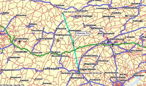
Map used with permission from DeLorme.
Figure 1. Map of South-Central PA showing Hawk Run, PA; Hagerstown, MD; and Orbisonia, PA. The latter test site is approximately 80 kilometers (km) from the reference stations.
At Orbisonia (designated R522), the researchers demodulated data from HRN2 and HAG1 using two demodulators. The user GPS antenna signal was split two ways, using an antenna splitter device, and then fed into two different laptop computers. One of the laptops received demodulated data from HRN2; the other received demodulated data from HAG1. Both laptops ran the application program, DynaPos.exeTM, in kinematic mode to achieve two separate RTK solutions for the user. During real-time processing, coordinates from HRN1 rather than HRN2 were used. Nevertheless, nearly correct baseline vector results were computed, although the results were offset. Therefore, this solution was reprocessed using the correct Hawk Run coordinates. Such reprocessing does not improve the accuracy because the data used in reprocessing was exactly the same data as that received in real time. This allowed the inadvertent setting to be corrected rather than requiring collection of new data. In other words, the reprocessed results are exactly the same as those that would have been achieved in real time if the correct reference station coordinates had been used.
HRN2, R522, and HAG1 are along a more or less north-south line, leading to the expectation of some systematic error cancellation in the north-south component when HAG1R522 and HRN2R522 are combined in a weighted average. Likewise, there would be little expectation of systematic error cancellation in the east-west component. The height error from HRN2 to R522 can be opposite that of the height error from HAG1 to R522 when there is a temperature and humidity gradient from HAG1 to HRN2. Consequently, the combined solution can benefit from error cancellation. An example of that would be a west-to-east moving thunderstorm. Such conditions were not observed on the day of the test.
Figures 2, 3, and 4 show plots for the north, east, and height components respectively. In all cases y = 0.0 represents geodetic truth. While the data were collected at a fixed location, the measurements were processed with medium dynamics; the Kalman filter had no knowledge that the site was static and assumed the antenna was moving several meters every second. Processing static data as kinematic with medium dynamics is a well proven and theoretically correct approach often used when it is not convenient to run a course and set up an additional local truth reference site.
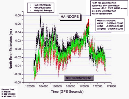
Figure 2. North component determined from HAG1 (black) and HRN2 (red), and the weighted average solution (green).
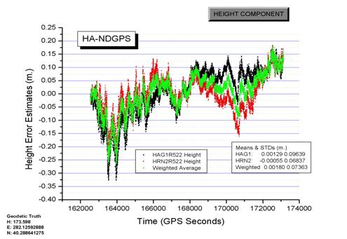
The north-south component benefited from the weighted average of the two solutions. This can be seen in the north-south plot as the weighted average solution appears to be closer to the truth. The east-west component in figure 3 did not appear to benefit from the combined solution; however, figures 5, 6, and 7 indicate both north-south and east-west component improvement. Thus, the benefit from averaging random errors might be greater than the benefit from systematic error cancellation. On the test day, height did not seem to benefit either. Note that near the end of the height plot Hag1R522 increased while HRN2R522 decreased. This opposite behavior becomes exaggerated in passing thunderstorms and hot, humid conditions where there is a gradient; a two-reference-station solution can reduce this significantly; however, this particular day was warm and calm.
This particular data experiment was almost too good to expect much benefit from weighted averaging. Normally there is a small random multipath reduction benefit from averaging user solutions from multiple reference stations. This is useful when baselines are short and multipath is the predominant error source. Every reference station to user solution will have a different reference station multipath; with enough reference stations, it might be possible to eliminate reference multipath. Unfortunately, this does nothing to reduce user multipath; therefore, after two or three reference stations are applied, the reference station multipath component becomes insignificant. In summary, there are both random error and systematic error components to reduce.
There is a more important error type to eliminate if possible-systematic error. For dual frequency processing, ionospheric delay errors are largely eliminated and tropospheric errors are usually the primary systematic error source. On the other hand, for single frequency DGPS, ionospheric path delay error is an important systematic error that can be reduced using multiple reference stations. Systematic broadcast orbit error contributions to position determination are on the order of 1 cm per 50 km, perhaps less, small when compared to the systematic error caused by tropospheric path delay (tropo), particularly in the user's vertical component. Thus, a primary reason to combine dual-band solutions based on different reference stations is the benefit from systematic tropospheric delay error cancellation.
For completion, figures 5, 6, and 7 show the east-north horizontal X-Y plots. These plots contain the same information as the north versus time and east versus time plots shown in figures 2, 3, and 4, but here they are presented in a more traditional manner where time is not explicit. The combined solution yields the better of the two solutions, seen in the tighter scatter plot in figure 7.
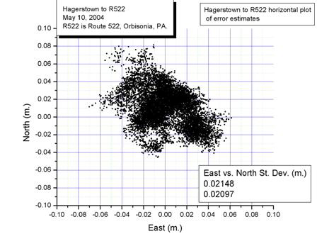
Figure 5. North component versus east component cross plot determined from HAG1.
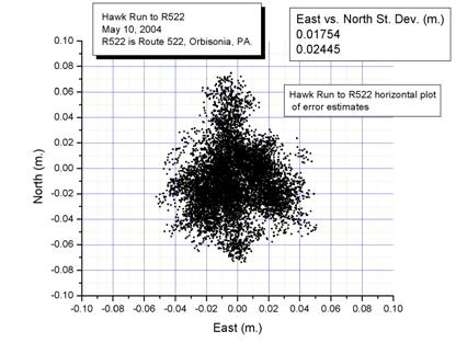
Figure 6. North component versus east component cross plot determined from HRN2.
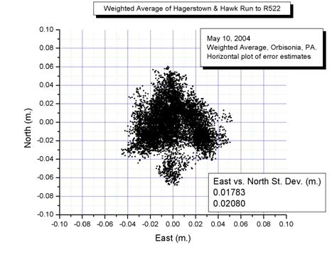
Figure 7. North component versus east component cross plot of HAG1 HRN2 combined.
The plot in figure 7 has somewhat better scatter properties resulting from the combination of the HAG1R522 and HRN2R522 plots. Under certain weather conditions, the combining of multiple simultaneous solutions can have an even greater improvement than experienced in this example.
Subtask 2e was to describe the algorithm used to combine independent solutions from Hagerstown and Hawk Run.
HAG1R522 and HRN2R522 solutions were combined as follows:
Let X1, Y1, Z1 represent the HAG1R522
solution at Orbisonia, PA.
Let X2, Y2, Z2 represent the HRN2R522 solution at Orbisonia, PA. For each of these six random variables, there is an associated standard deviation (i.e., σ) output from the two Kalman filters. The following equations describe the algorithm used to combine solutions:
 (1)
(1)
 (2)
(2)
 (3)
(3)
This algorithm does a fair job of combining solutions and giving the better solution component more weight. (A simple alternative that could be used, but which is generally not recommended, is to average the solutions for all the participating reference stations.
This simple solution will be reasonable as long as all the Position Dilution of Precisions (PDOP) are in reasonable agreement; however, if the PDOPs differ greatly, this procedure should be avoided.) The combining of standard deviations to achieve a single standard deviation is more problematic because the correlated nature of systematic errors has not been developed. The current method is simply to take the smaller of the two standard deviations. Combining solutions from two reference stations yields a 13.4 percent reduction of random component error, which continues as reference stations are added. With enough reference stations, this random component reduction can be as great as 29.3 percent. For traditional code DGPS users, this would be welcome because code multipath can be several decimeters to meters in magnitude. For carrier-based RTK users, reduction of this relatively small component is not of great help.
On the other hand, the code plays an initial role in RTK, so that multiple reference stations speed up initial convergence because of this random reduction factor. After steady-state is reached, reduction of reference station carrier multipath is not as important as systematic error cancellation of tropo, iono, and orbit error. As stated above, orbit error is quite small, and iono error is essentially eliminated by forming iono-free combinations of measurements. This leaves tropo error as the most problematic systematic error source. Activities are underway at National Oceanic and Atmospheric Administration (NOAA)/National Geodetic Survey (NGS), USCG/Command and Control Engineering Center (C2CEN), and NOAA/Forecast Systems Laboratory to develop real-time data that can be broadcast to RTK users to reduce the tropo path delay errors. This can take the form, for example, of wet zenith delays relative to the broadcast site. (Note: Reference station-to-user distance weighting was not used in the combining algorithm, and it might be a consideration, depending on the Kalman filter assumptions.)
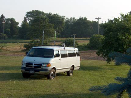
The photograph in figure 8 shows the configuration of the van used in this test. Two demodulator antennas were used-one received HAG1 broadcast XCOR messages, the other received HRN2 broadcast XCOR messages. The van's local GPS antenna, located in the back on the driver's side, was fed to a signal splitter and subsequently input to separate laptop computers. The fourth antenna shown in the photograph, located just above the driver, is unrelated to this test.
Task 3, to develop and implement a prebroadcast integrity algorithm, had several aspects.
Subtask 3a was to detect errors in the GPS constellations and its broadcasts. The coordinates of the reference site are ostensibly known. In practice, this was a minor point of confusion during the research and development phase. It is possible to broadcast data from HAG1 but wrongly supply coordinates for HAG2. This is just one integrity reason why the local point-position solution should be checked when the configuration of the HA-NDGPS reference station is changed. While point-positioning solutions are not highly accurate, it is usually possible to discriminate between reference station sides by inspecting the GRIM point solutions as part of any setup procedure.
Adding reference station code corrector-type residuals for integrity is a possible solution. Generally a residual is the difference between something expected and something actual. For example, it is possible to compute a GPS range based on a geodetic location and a satellite location. The actual measurement may differ by a few centimeters, which is the residual, or the left over amount. Large residuals indicate poor measurements, poor orbits, or incorrect geodetic coordinates, or other problems. Small errors are a necessary but not sufficient condition for integrity. Subtask 3b begins to address this issue. The site technician or the control station operator must verify that code residual errors are within specified tolerances.
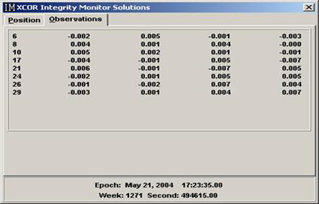
As an example, compare the two screen shots shown in figures 9 and 10. In figure 9, the correct coordinates were used; in figure 10, the wrong coordinates were used. The intentional error in figure 10 was 100 meters in each component. There are large positional errors (top three lines) and large residuals (lower lines below section divider line) caused by wrong coordinates.
Figure 10. An example screen shot of prebroadcast positional integrity with the wrong coordinates.
These large residuals indicate an error with the reference station coordinates. This could be extended to a differential check by using data from a second NDGPS GPS receiver as a prelude to accepting the modulated message for transmission to users. In differential mode, the code DGPS residuals would be about 1 m and NDGPS Integrity Monitor (IM) residuals are about 1 meter. In local RTK differential mode, all of the two-station, two-satellite carrier double differences are expected to about 1 cm.
An unpack feature has also been added to the message formation process. After forming XCOR messages to be broadcast to users, but before the actual broadcast is consummated, the software unpacks the message and compares it with the original data.
Figure 11 shows a comparison of original data with the unpacked data at the reference station before broadcasting the data to users. This comparison allows the reference station to evaluate what will be sent to the user. Unpacking the message before it is broadcast provides the opportunity to catch a problem and prevent the transmission of bad data.
Subtask 3b was to discuss methods of inserting integrity information into the data stream.
One method that has been considered for inserting integrity information into the data stream is to provide a single bit to indicate an integrity message in the data stream at a fixed and known location. The integrity message length would be variable to allow expanded integrity messages. Four to eight bits would be required to accommodate a suite of possible messages, including some combinations. Following are some possible messages:
0-Unreliable; do not use
1-Test and evaluation use only.
2-Code and carrier positioning use.
3-L1 only code navigation use.
4-Multifrequency code navigation use
5-General code and carrier navigation use.
6-Change of site coordinates, caution.
Subtask 3c was to suggest possible techniques and algorithms. This includes unpacking messages before transmission and verifying that unpacking returns the original data. It also includes verifying that one-way code residuals are small. It also includes verifying that point-positioning solutions agree with a priori known reference station coordinates. This is similar to subtask 3a.
Integrity monitoring could be dramatically enhanced by exploiting the availability of the NDGPS IM receiver or any other local receiver. Even a non-local GPS receiver could be used through network scenarios. The data from a second receiver could be ingested into the reference station software for code and carrier positioning in RTK mode. If the second receiver is on the same reference station site (for example, within 100 meters of the primary reference receiver), then the baselines are short and individual solutions could be performed for each data type. Currently that would comprise R1 and R2 code solutions and L1 and L2 carrier solutions. The carrier solutions could be of two varieties-float and fixed. With these solutions, the correct vector and second site coordinates would be necessary conditions, or there is a problem such as the sites might be confused. The code solutions would be accurate at the 1-meter level; fixed RTK solutions would be accurate at the 1-cm level on an epoch independent basis. Float RTK solutions would converge slowly like a distant user. Residual computations can provide an equally powerful validation of the data. The discussion of subtask 3a also addresses residuals.
Task 3 covers four types of integrity solutions: point positioning, code differential, carrier differential, and IM single-epoch solution.
Task 4 had several aspects.
Subtask 4a was to convert the demodulated output format into RTCM 18/19 compatible with existing user GPS equipment.
A new software module, HAtoRTCM.EXE, translates the GRIM-demodulated XCOR message into messages RTCM 18 and 19. These messages are compatible with existing RTCM 18 and 19 compatible user equipment.
The outputs of this module were studied in two different ways. In the first effort, RTCM 18 and 19 messages were converted into Receiver Independent Exchange (RINEX) format and compared with the original data before RTCM 18 and 19 formation. These data compared correctly.
The second and more practical method of testing was to output these RTCM 18 and 19 messages from a PC comport into RTCM 18/19-capable user GPS equipment. For this test, existing dual frequency GPS receivers were used. The receivers needed to be configured according to the user manual. This specific receiver has an installed "Carrier Phase Differential Remote RTK" option, ideal for such a test. The receiver RTK positioning results were output to a different RS-232 port and returned to the original PC that formulated the RTCM messages, which then were sent to the receiver. The returned results were gathered using the data-capture function of a terminal emulation program such as the Thales Navigation's Micro-ManagerTM Pro, Remote32 software, or Terminal Window program. Any commercial terminal window program could be used to capture this data as well. The plotted captured data are shown in figure 12.
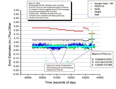
Figure 12. Demonstrated proof that GRIM to RTCM 18/19 works.
These results show that RTCM 18 and 19 capable user GPS receiver equipment accepted these messages and performed RTK positioning. To test the capability somewhat further, the RTCM 18/19 stream was intentionally disconnected and reconnected. These breaks show up in the plot in figure 12. The number of satellites (divided by 100) and the PDOP (divided by 10) are included in the plot.
In the discussion of Task 4, there is only one method of access to the HA-NDGPS signals: demodulator receiver to GRIM, GRIM to HAtoRTCM.EXE, HAtoRTCM.EXE to user GPS receiver, and GPS receiver output to user application.
There are currently two other methods available for test and evaluation of HA-NDGPS broadcasts. The first is GRIM RINEX output. GRIM records the real-time HA-NDGPS messages bit for bit in a trap file. Simultaneously (but optionally) GRIM will convert these compressed messages to user-friendly text RINEX files. While the RINEX files would be processed in post-mission mode, this approach enables all users to have a role in the test and evaluation phase.
The next method of access concerns application developers. A GRIM developer's kit is available from The XYZs of GPS. The kit provides direct and real-time access to the demodulated and decompressed broadcast message data, without the need to convert to an intermediate standardized format such as RTCM 18/19.
In summary, currently three methods are available for test and evaluation of HA-NDGPS messages.
Task 5 had several aspects.
Subtask 5a was to rewrite the existing modulator interface to implement a remote control capability through a TCP/IP interface. The modulator interface was rewritten so that the HA-NDGPS reference station software could be controlled from NAVCEN. At the time of this report, the complete suite of network equipment ordered by the government had not arrived, so testing of the software had to be carried out using a temporary network. The testing was fully successful.
The remote control capability allows substantial configuration control of the HA-NDGPS reference station. Most changes that currently require a visit to the site will be possible from NAVCEN. For the Hagerstown site, this will be convenient; for the Hawk Run site and planned additional sites further west, this will prove to be indispensable. These commands include software and hardware resets, broadcast measurement definitions and bit rates, and more. All commands are documented in the High Accuracy Control Program (HACP) manual; there are several dozen commands. The following command and response syntax has been excerpted from the HACP manual:
The HACP TCP/IP protocol is an NMEA-like messaging structure that is ASCII based (and is similar to that used by the GPS receivers). The general forms are:
Query
$PXYZQ,type[*XXXXXXXX] <CR><LF>
Response
$PXYZR,type[,data][*XXXXXXXX] <CR><LF>
Command
$PXYZS,type[,data][*XXXXXXXX] <CR><LF>
Notes: 1. Those items enclosed in "[" and "]" are optional.
2. <CR><LF> represent the carriage return/line feed sequence.
As a protocol rule, every command that begins with $PXYZS,type will have some type of response. Some commands will have a direct response with the command name in them. Others will have either a $PXYZR,ACK,type (for acknowledge), $PXYZR,NAK,type (for negative acknowledge), or $PXYZR,UNS,type (for unsupported "type" message).
Note: In the protocol descriptions that follow we do not show:
1) The trailing <CR><LF> sequence that follows each message.
2) The optional 32-bit CRC (in the form of *XXXXXXXX).
In this Phase II effort, the command set is extensive and allows an operator to query and command essentially all aspects of the HA-NDGPS operation. Following are a few specific examples:
What version are you?
Query: $PXYZQ,RID
Response: $PXYZR,RID,s1,s2,s3
GRIM, what is your status?
Query: $PXYZQ,PRG,GRIM
Responses: $PXYZR,PRG,GRIM,RUN
GRIM is currently running
$PXYZR,PRG,GRIM,NORUN
GRIM is present but not running.
$PXYZR,PRG,GRIM,STOPPING
GRIM is present, it's running, but has been commanded to stop.
$PXYZR,PRG,GRIM,ERR
Cannot find GRIM program.
Subtask 5b was to add limited commands to control GPS receiver parameters (e.g., data rate and elevation mask).
In addition to controlling the HA-NDGPS software to configure the broadcast message, changes may be required for associated GPS receiver hardware configuration. Examples of parameter that can now be commanded from NAVCEN are the elevation mask and the observation epoch spacing, as illustrated here:
What is the recording interval?
Q: $PXYZQ,GNI,REC_INT
R: $PXYZR,GNI,REC_INT,current_interval
C: $PXYZS,GNI,REC_INT,new_interval
What is the elevation mask?
Q: $PXYZQ,GNI,EL_MASK
R: $PXYZR,GNI,EL_MASK,f1
C: $PXYZS,GNI,EL_MASK,f1
Following is an example of an operator query for station coordinates, a status response, and a reset for new values:
Q: $PXYZQ,GNI,COR_REF_POS
R: $PXYZR,GNI,COR_REF_POS,d1,f1,f2,f3
C: $PXYZS,GNI,COR_REF_POS,d1,f1,f2,f3
The software developed to accomplish Task 5 includes an updated modulator interface and HACP. HACP is the primary software to handle configuration changes and distribute those changes to other software to carry out the changes.

