U.S. Department of Transportation
Federal Highway Administration
1200 New Jersey Avenue, SE
Washington, DC 20590
202-366-4000
Federal Highway Administration Research and Technology
Coordinating, Developing, and Delivering Highway Transportation Innovations
 |
| This report is an archived publication and may contain dated technical, contact, and link information |
|
Publication Number: FHWA-HRT-05-034
Date: July 2005 |
Task 6 had several aspects.
Subtask 6a was to collect data at reference station REMD (at 1 Hz) in Dickerson, MD, and user location MAST (also at 1 Hz) in Dover, DE. The distance between the two stations was approximately 180 km. The data were processed in RTK float mode to achieve decimeter heights and half-decimeter horizontals. The data used were full dual carrier and code observations such as those broadcast from HA-NDGPS reference stations.
The first RTK run (1 Hz; 1 Hz) was compared with a priori known truth (millimeter accuracy). The kinematics assumed in all runs were set at 1 m/s in all components, known as "velocity surprise" because it represents how much the velocity can change in one second. This level would be satisfactory for a car traveling on the highway or a hydrographic survey vessel on the Chesapeake Bay. The actual kinematics are unimportant because this is a study of errors created at the static reference site. Data were reprocessed using 5-second REMD epochs and 1-second MAST epochs.
Of interest is how the trajectory changes as a result of the thinning of the reference station data (REMD) caused by a reduction in bandwidth. For example, when the bandwidth changes from 1,000 bits per second(bps) to 200 bps, the broadcast message takes 5 times as long to arrive, and it cannot be applied for user processing until 5 seconds after the data were observed. In addition, the user must continue to use the latent data for another 4 seconds. (i.e., use the same reference station broadcast measurements, predicted forward, for 4 additional seconds.) In a typical RTK scenario, a user would use the data from 5 seconds to 9 seconds old. If a broadcast message is corrupted by background noise and needs to be discarded by the user, use of the data would continue beyond 9 seconds old, up to 14 seconds old. After a gap, the full accuracy is returned immediately.
This is considered a typical RTK scenario. Other scenarios are available to users, depending on the mission. For example, it is possible for a user to hold off processing by 5 seconds and process only time-aligned data. Another example is to process with 5 seconds of latency and set an inertial unit. In this scenario, the expectation is that the inertial unit would be more accurate than GPS.
Figure 13 shows the percentage of data collected and its availability for use. Between 0 seconds and 4 seconds, the data are broadcast to the user, who must wait nearly 5 seconds for the bit-by-bit broadcast to be completed and the data packet to be received and demodulated before it can be exploited. The user cannot use this packet until the entire packet has been received because the message in full must pass the parity check before the user can trust it. The full packet needs to be gathered and recognized, at least in the current design, before sending it to the parser and the interpreter, all before passing it to the user application. In the figure, the data collected at second 0 did not begin to be used by the user application until second 5; the user continued to use the 0-second data until 9 seconds. The figure shows a 1-second user scenario. If the user was instead a 10 Hz user, the data would be used until 9.9 seconds, more or less. By second 10, the measurements collected at second 5 have fully arrived and can now be exploited for the subsequent 5 seconds.
Figure 13. Percentage of data collected 0 to 10 seconds for 25 epochs.
Figure 14 shows a comparison of the RTK solution (180 km) with millimeter truth after an initial convergence period, which is not shown. The north-south and east-west components are better than 5 cm where the height is good to about 1 dm. This "1-second REMD, 1-second MAST" RTK solution is referred to throughout the Task 6 discussion, giving a basis of comparison for the lower-bandwidth (thinned) scenarios that follow. Figure 15 shows a comparison of the 1-second REMD, 1-second MAST (1,000 bps) RTK solution (180 km) with the 5-second REMD, 1-second MAST (200 bps) RTK solution.
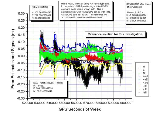
Figure 14. Expected HA-NDGPS performance at 180 km.
Figure 15 represents the change that results solely from the reduced bandwidth rather than the error penalty suffered when compared with millimeter truth. The additional error caused by the bandwidth reduction and the associated increased latencies is about 0.25 dm. Table 1 compares this 5-second scenario against millimeter truth. Comparing these statistics with the 1-second broadcast scenario in figure 14 (i.e. means plus standard deviations) shows there is no significant accuracy performance degradation when data are broadcast based on 5-second epochs. (The means and standard deviations are essentially the same.)
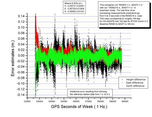
Figure 15. Comparing 5-second broadcast with 1-second broadcast from HAG1.
Table 1 indicates there is little difference between the 1-second, 1-second scenario and the 5-second, 1-second scenario when compared to millimeter truth. The means (−40 mm, −1 mm, 17 mm) are similar to those shown in figure 12 (-46 mm, 4 mm, 13 mm). The standard deviations (68 mm, 25 mm, 25 mm) are almost identical (68 mm, 24 mm, 24 mm).
Table 1. Accuracy performance of 5-second broadcast scenario.
| Component |
Means (mm) |
Standard Deviations (mm) |
|---|---|---|
| Height |
−40 |
68 |
| East |
−1 |
25 |
| North |
17 |
25 |
Next is the 10-second REMD, 1-second MAST scenario. Obviously the bandwidth would be halved and the latencies would be doubled. Increasing the epoch spacing clarifies how much degradation could be expected as a result of missed messages. For example, when operating a reference station at 5-second epochs, suppose a user misses an epoch. In that case, the prior received message would be used for a total of 14 seconds rather than the normal 9 seconds. This motivates the study of 10-second, 15-second, and 20-second scenarios that soon follow. Following are the results of the 10-second/1-second scenario.
Figure 16 shows the error that results from broadcasting REMD data at a 10-second rate versus a 1-second rate. The added error is still smaller than the absolute error and suggests only moderate error growth when the 5-second, 1-second scenario experiences one or two missed epochs at MAST. Clearly when there are no missed messages in the 10-second, 1-second scenario, the results are still good. Even in the 10-second scenario, some positioning users will be satisfied with processing 10-second aligned epochs roughly 10 seconds late.
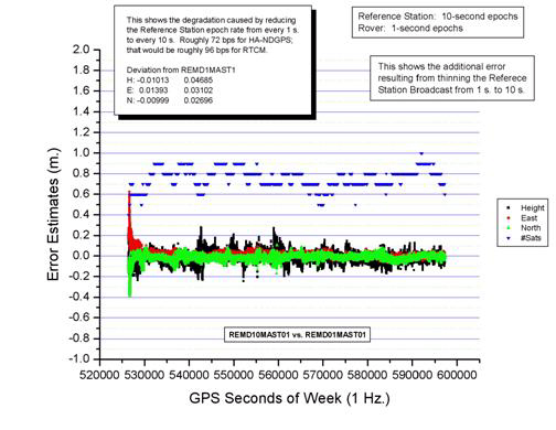
Figure 16. Comparing 10-second broadcast with 1-second broadcast from HAG1.
Table 2 shows how this 10-second, 1-second RTK scenario compares with millimeter truth. Compare these statistics with the 1-second broadcast scenario shown in figure 14 to see only a 10 percent accuracy performance degradation when data are broadcast based on 10 second epochs.
Table 2. Accuracy performance of 10-second broadcast scenario.
| Component |
Means (mm) |
Standard Deviations (mm) |
|---|---|---|
| Height |
−38 |
73 |
| East |
−6 |
26 |
| North |
21 |
29 |
Clearly the absolute error in the horizontals has grown from the half-dm level to the dm level. Most of this increase results from using the 10-second broadcast up to 19 seconds past user-time-aligned data.
Following is the 15-second, 1-second scenario, which suggests that while the error indeed increases, the error growth is still gradual. Figure 17 shows a comparison of the 15-second, 1-second scenario with the original 1-second, 1-second scenario. The error shown is the result caused solely by thinning the data broadcast to 15-second epochs, and it reflects the increased latencies. The absolute error associated with this case is shown in table 3. Compare these statistics with the 1-second broadcast scenario in figure 14 to see the possibility of 50-percent accuracy performance degradation when data are broadcast based on 15-second epochs.
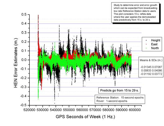
Figure 17. Comparing 15-second broadcast with 1-second broadcast from HAG1.
Table 3. Accuracy performance of 15-second broadcast scenario.
| Component |
Means (mm) |
Standard Deviations (mm) |
|---|---|---|
| Height |
−34 |
92 |
| East |
−6 |
36 |
| North |
22 |
36 |
Clearly the error increase is significant and undesirable. The 1 Hz rover solutions were generated using reference station data that were from 15 to 29 seconds old. Nevertheless the error growth has been gradual.
Figure 18 shows the 20-second, 1-second scenario where a typical RTK user at 180 km would begin to use the broadcast data after 20 seconds and end the use after 39 seconds. To be clear, the user would re-use a single broadcast epoch, in a predictive sense, for roughly 19 seconds (after already waiting 20 seconds to get it).
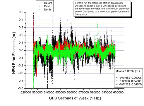
Figure 18. Comparing 20-second broadcast with 1-second broadcast from HAG1.
The horizontal error resulting from the reduced bandwidth remains less than 1 dm. Table 4 compares the results of the 20-second, 1-second scenario compared to millimeter truth. Compare these statistics with the 1-second broadcast scenario in figure 14 to see the possibility of 100-percent accuracy performance degradation when data are broadcast based on 20-second epochs.
Table 4. Accuracy performance of 20-second broadcast scenario.
| Component |
Means (mm) |
Standard Deviations (mm) |
|---|---|---|
| Height |
-32 |
106 |
| East |
-9 |
40 |
| North |
26 |
44 |
These results suggest that 144 bps is minimally adequate for broadcasting dual GPS code and carrier data to a user under nominal levels of ionospheric activity, which affects the GPS signals, and nominal levels of atmospheric noise, which affects the data link. While 144 bps might be adequate to meet a simple local or private need, it would not be adequate to serve the public. First, the 144 bps rate supported 9 GPS satellites, but 12 satellites would be expected. Second, position and site name should be broadcast approximately once every 4 epochs rather that once per 60 epochs. Third, a set of smaller packets would constitute a more robust broadcast rather than the current one packet (all or nothing) message. Fourth, the addition of an integrity message would require several more bits. These four points would bring the broadcast rate to possibly 200 bps. Next, include L5 code and carrier measurements. For 12 satellites, this would require possibly 600 additional bits over 5 seconds or 120 bps, perhaps less. In addition, it might be possible to include additional information such as tropospheric zenith delay parameters, ionospheric zenith delay parameters, or precise orbit parameters, or all of these. Although the incremental bandwidths for these are difficult to estimate at this time, the following paragraph describes the first estimates.
The first estimates are 900 bits for a tropospheric delay grid or 25 bps for 3 minutes at 5-second epochs. The precise orbits might take 60 bps over 3 minutes at a 5-second rate. To repeat, these estimates cannot be accepted as conclusive. An ionospheric delay grid would be less dense, but it would require a wider range of values. A first rough estimate might be 45 bps. These estimates sum to 450 bps, assuming a 5-second broadcast. It is possible that the broadcast of precise orbits would never be required because those orbits broadcast directly from the GPS satellites are accurate to 0.25 mm per km from the reference station. This causes a random positioning error of about 6.25 cm at 250 km. Orbital improvement underway will reduce that error by a factor of about 2.5, leaving a random positioning error of about 2.5 cm at 250 km. Also, with dual data, an ionospheric delay grid serves a limited user population; therefore, it may not be required. Clearly a tropospheric delay grid has the most potential value to users.
In summary, 500 bps should be adequate to serve the public for GPS alone. If there is a decision that orbital data or ionospheric delay data do not have sufficient value, the remaining bandwidth would best be used by increasing the broadcast frequency from once every 5 seconds to as often as possible, which would be more or less once every 3 seconds.
There are smaller parent/child packet messages that have been laboratory tested, but they have not been evaluated for HA-NDGPS. To date broadcasts have been single packet where an entire epoch is broadcast in a single packet such as the RTCM-104 Type 1 message. These multipacket formats have some additional overhead, but the odds would be increased of message packets reaching distant users. Although smaller multipacket (parent/child) formats have not been exercised in the field, it is anticipated that they will be field tested in the months ahead.
In general, data gaps do not cause unusual problems. When data packets are missed, the previous packet continues to be used, much as RTCM Type 1 or Type 9 messages would continue to be used. If data packets are missed, a gradual increase in positioning error results, as demonstrated above. When the next packet arrives and passes the cyclic redundancy code (CRC) check, full accuracy returns to the user. Nevertheless, it is important that distant users experience a minimum number of missed packets.
Task 7 had several aspects.
Subtask 7a was to collect data for mapping one or more highway segments. Researchers traveled Route 15 north of Frederick, MD, on two separate driver analysis runs. In each run, there were eight to nine loops of 12 miles or more. Because the van could maintain the same lane, sections of roughly 4 km northbound and roughly 4 km southbound were used. Figure 19 shows a map section of U.S. Route 15 north of Frederick, MD, where the test took place.
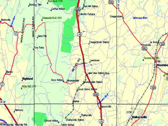
Map used with permission from DeLorme.
Figure 19. Map segment of test site along U.S. Route 15 north of Frederick, MD.
The real-time motion plot in figure 20 shows a sample of the highway. Visible are nine passes over this section of Route 15. The blue icon shows where the van is (current track) on a rerun of the data. Figure 21 shows that the driver was able to repeat the track to within 14.5 cm root mean square (rms).
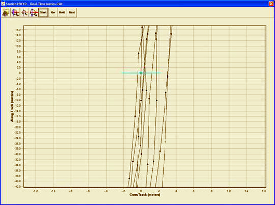
Figure 20. Display of nine tracks driven on U.S. Route 15 north of Frederick, MD.
From these runs, researchers created the road "definition" using the same program that was used to process the measurements. Figure 21 shows a small segment the roadway created manually as a visual average of the nine loops.
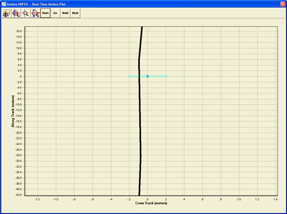
Figure 21. Display of defined "road map" created from nine tracks in Figure 20.
It is also possible to show all nine loops superimposed on the roadway.
The roadway was determined in float processing mode, and it is probably accurate at the 5-cm level after the first two loops. The positioning program could have determined the roadway precisely (1 cm) with a local reference station and subsequently operated in real time based on the Hagerstown broadcast. This was not done. For this test, the HA-NDGPS broadcast was used both to create the map and determine the driver's tracks on the same map.
Subtask 7b was to compare the driver's control of the vehicle. Figure 22 shows the driver's cross-track history related to the created road map. The figure shows the cross-track distances from the mapped road when the van was on the northbound and southbound segments of each loop. The gaps represent the portions of the loops where repetition was not possible because of a concern for traffic safety.
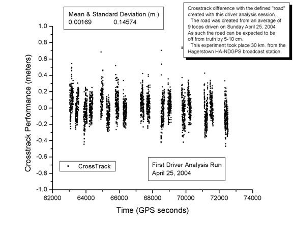
The following method was used to compute the cross-track quantity. First the "road" was defined to be the average of the nine tracks; the average was generated visually. Because there were nine tracks, the visual procedure tended to ignore an obvious outlier. The end result of defining a road is a set of geodetic coordinates. Also, the points on the nine tracks have geodetic coordinates. The road points can be transformed to a local X-Y-Z topocentric frame where this frame is aligned with north (N), east (E), and the perpendicular to north and east, ellipsoidal height (H). Now individual points on the nine tracks could be converted to this topocentric frame and compared with the closest point in the set of road points. This was done, but the result is of little interest to compare the NEH of the tracks with NEH of the road. One more transformation computed the relative azimuth of two consecutive points on a track, then rotated the topocentric frame by this azimuth angle. This new frame is aligned along track and the closest point on the road is rotated into this new frame. While along-track and height were used to define this new frame, there is a cross-track component byproduct. In this frame the cross-track of a track point is zero and the cross-track of the nearest road point is plus or minus (i.e., left or right). This cross track component of the road with respect to the point on a track is the quantity presented in figure 22.
This route was traveled a second time with generally the same results. When the road generated from the first driver analysis run was applied to the second driver analysis run, the cross track behavior was 20 cm compared to 15 cm, an expected result. Clearly the roadway would be better defined based on many runs from different days and different satellite constellations. Obviously, it could have been determined better (i.e., 1 cm) with a local (e.g., within 5 km) reference station and centimeter RTK processing; however, this was not done.
The photo in figure 23 shows the van configuration for the Route 15 driver analysis runs. No attempt was made to place the user's local GPS antenna along the center of the van.

Figure 23. Van configuration used for driver analysis on U.S. Route 15.
Task 8 had several aspects. Subtasks 8a and 8b are discussed together.
Subtask 8a was to locate a GPS antenna high above possible nearby multipath sources and compare the cleanliness of the measurements there with measurements from current NDGPS equipment. Subtask 8b was to use similar antennas, at both reference and a nearby user site, to gather observations and fix the integers to establish the level of site cleanliness.
A machine shop fabricated a pentapod apparatus to install high above the Hagerstown HA-NDGPS site to provide a signal as clear of multipath as could be done easily. This allowed researchers to compare signals with the existing NDGPS antenna locations.
Figure 24 shows a photo of the Hagerstown facility with the pentapod located on the roof and the HAG2 NDGPS GPS antenna protective dome in the background to the right.
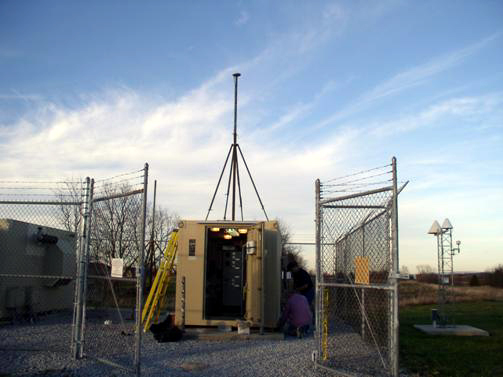
Figure 24. The Hagerstown GWEN site with a pentapod marine antenna 4 to 5 meters above the hut to search for the cleanest signals.
At first researchers selected HAG2 to be the HA-NDGPS antenna and receiver. In this case, the antenna was a 700829 (3) Ashtech® antenna coupled with an NDGPS Z12R RS (reference station) GPS receiver. The van was instrumented with an antenna as shown in figure 25.
Figure 25. Van configuration for multipath testing at the Hagerstown GWEN site for the NDGPS 700829 (3) antenna from Ashtech to van 700829 (3) antenna from Ashtech test.
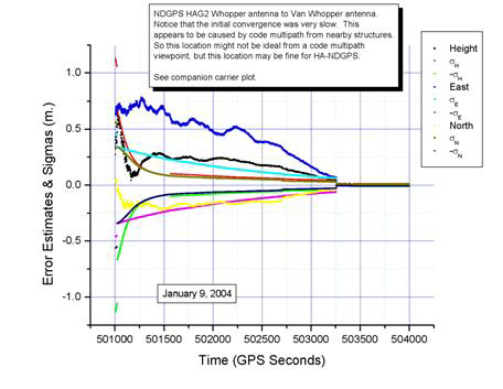
Next, researchers collected HA-NDGPS broadcast messages from HAG2 and processed the data as shown in figures 26 and 27. Initial convergence was slower than usual (figure 26); researchers interpreted this to indicate there was significant code multipath. Later in the processing, there was adequate convergence to fix the ambiguities to integers (figure 27). In that case, the results were stable; researchers interpreted this to mean the carrier multipath was not a factor and the 700829 (3) antenna from Ashtech geodetic antenna provided excellent carrier measurements.
Next researchers used the Ashtech 700700 (B) marine antenna on top of the hut as the HA-NDGPS antenna plus an Ashtech Z12 Real-Time Sensor GPS receiver. The van was also configured as shown in figure 28.
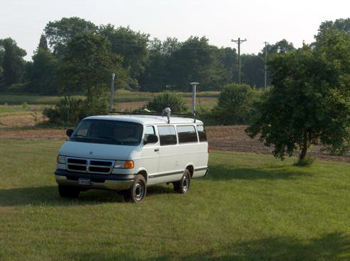
Figure 28. Van configuration used for multipath testing at the Hagerstown GWEN site. In this case, HA-NDGPS marine antenna to van marine antenna is under test.
In this case, the initial convergence seemed to be nominal, as shown in figure 29. Researchers interpreted this to mean there was not as much code multipath at the marine antenna high above the hut as was experienced by the NDGPS antenna.
Figure 29. HA-NDGPS marine antenna to van marine antenna initial convergence.
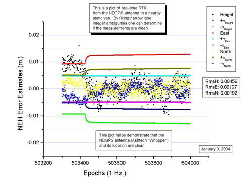
After the results converged sufficiently to fix ambiguities to integer values, the integers were fixed, as shown in figure 30. The solution with integers fixed looked similar to the integer fixed solution using the 700829 (3) antenna from Ashtech. Researchers interpreted this to mean both sites were clean with respect to carrier multipath.
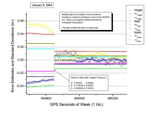
Figure 30. HA-NDGPS marine antenna to van marine antenna steady state with integers fixed.
In summary, NDGPS sites appear to have high-quality carrier observations. On the other hand, the NDGPS site code observations might have experienced significant multipath. Potentially, this is an issue if users use HA-NDGPS signals for code range navigation. It is also potentially an initialization issue for HA-NDGPS users because HA-NDGPS users will depend on the code observations during the early seconds or minutes to provide aiding to the carrier measurements.
It is significant that when NDGPS 700829 (3) antenna from Ashtech antennas are mixed with 700700 (B) marine antennas, the results are not good unless antenna modeling similar to that performed by NOAA and NGS is included.
The research in this task was directed toward proving system capabilities, examining possible applications, and refining various system functions. The effort was very successful in all three areas.
Task 2-Modulator Software Rewrite and Multiple Station Solution. The new modulator software performed with greater reliability than the previous version. By supplying the modulator with data before the buffer was empty, the broadcast did not drop bits due to the nondeterministic effects of the operating system. The improvement in performance using two sites to determine the users' navigation solution gained from this relatively simple weighting implementation provides solid proof that multiple reference stations offer improved performance. More complex implementations that are currently available offer even greater benefits.
Task 3-Prebroadcast Integrity Algorithm. Development of the integrity approach offers significant insight into to the best way to implement this feature. It provides subsecond indications to the users of solution problems. Shortly thereafter, users receive an indication of the problem so they are able to apply the information and generate a navigation solution. While further work to refine the user alerts is needed, this early effort has proven successful in meeting our requirements of notifying users of satellite usability.
Task 4-RTCM Data Output. This capability allows the system to operate with almost any GPS receiver on the market today, giving users an easy way to develop applications using existing components. As new demodulators are developed, this software can be built-in to provide greater flexibility and easier implementation.
Task 5-Modulator Interface. This provides greater remote control capability, reducing the need to visit sites on a regular basis. Its implementation provides significant benefits as more geographically distant sites are installed.
Task 6-Low Baud Rate Messages. This task demonstrated the ability of the system to provide information at even lower data rates and offers insight into what the minimum data rate should be, given the parameters at the time of the test. Data rates as low as 100 bps will work, but higher data rates are needed to ensure the user received adequate and low latency information to make an accurate navigation solution.
Task 7-Highway Application. The ability to use a real-time solution to demonstrate driver behavior offers benefits, but further exploration is needed to quantify the benefits. Task 7 was intended to begin that process and did so successfully by illustrating the type of information that could be gathered and analyzed.
Task 8-Noise. Quantifying the noise at Hagerstown and demonstrating the stability of the reference stations, and insight into the effects of taller reference station towers and multipath can be further explored to reduce their effects at other sites.

