• Federal Highway Administration >
• Publications >
• Research Publications >
• 09049 >
• Nondestructive Evaluation >
• The Effects of In-Vehicle and Infrastructure-Based Collision Warnings at Signalized Intersections

The Effects of In-Vehicle and Infrastructure-Based Collision Warnings at Signalized Intersections

PDF Version (888 KB)

PDF files can be viewed with the Acrobat® Reader®

Table of Contents

Foreword

The Federal Highway Administration (FHWA) Office of Safety Research and Development is focused on improving highway operations and safety by increasing the knowledge and understanding of the effects of intersection design on operational efficiency and safety. Intelligent Transportation Systems (ITS) have been shown to have both safety and operational benefits. ITS is a worldwide initiative to incorporate communications and information technology in transportation systems. This study was conducted to investigate the potential for an ITS countermeasure to reduce the number of collisions that result from red light violations at signalized intersections. In the United States, red light violations have resulted in over 1,000 fatal crashes per year for many years. The research reported here examined the potential effectiveness of warnings to prevent such crashes.

Raymond A. Krammes
Acting Director, Office of Safety
Research and Development

Technical Documentation Page

Form DOT F 1700.7 (8-72) Reproduction of completed pages authorized

SI (Modern Metric) Conversion Factors

Table of Contents

• Introduction
  • Objectives
  • Background
• Approach
  • Conditions Tested
  • Infrastructure-Based Warning
  • In-Vehicle Warning
• Combined Infrastructure-Based and In-Vehicle Warning
• Participants
• Research Design
• Protocol
• The Driving Simulation
• Results
• Amber Signal Responses
  • Response Time
  • Peak Deceleration
• Warning Responses
  • Warning Onset
  • Warning Effectiveness
  • Warning Response Time
  • Peak Deceleration
• Discussion
• Driver DecisionMaking at Onset of the Amber Change Interval
• Warning Effectiveness
• Recommendations
• References

List of Figures

• Figure 1. Screenshot. Simulated signalized intersection with activated infrastructure-based red light violator warning
• Figure 2. Screenshot. Simulated signalized intersection in normal operation
• Figure 3. Graph. Brake pulse acceleration as a function of time shown relative to the onset of the voice message and red LED on dashboard
• Figure 4. Graph. Degrees of pitch in simulator cab as a function of time during in-vehicle emergency warning event given no driver input
• Figure 5. Screenshot. Left outside and center-mounted rear view mirrors viewed from behind the vehicle
• Figure 6. Screenshot. Other car leads condition
• Figure 7. Equation. Calculation for the TTSL_W
• Figure 8. Graph. Frequency distribution of the number of stops required by participants to complete the modified method of limits procedure
• Figure 9. Graph. Distribution of the means for the TTSL decision points
• Figure 10. Graph. Mean within participant variability in speed as a function of car-following conditions
• Figure 11. Graph. Mean TTSL for amber signal decision as a function of assignment to warning and car-following conditions
• Figure 12. Graph. Mean of average accelerator release and brake response latencies as a function of car-following conditions
• Figure 13. Graph. Accelerator amber onset response latency distribution
• Figure 14. Graph. Brake amber onset response latency distribution
• Figure 15. Graph. Estimated population percentiles for accelerator and brake response times calculated using a lognormal transformation
• Figure 16. Graph. Distribution of TTSL for initiating the warning
• Figure 17. Graph. Percentage of drivers delayed by a least 1 s in arrival at an intersection after the onset of an infrastructure-based warning
• Figure 18. Graph. Percentage of drivers delayed by a least 1 s in arrival at an intersection after the onset of an in-vehicle warning
• Figure 19. Graph. Percentage of drivers delayed by a least 1 s in arrival at an intersection after the onset of simultaneous infrastructure-based and in-vehicle warnings
• Figure 20. Graph. Accelerator release response times following the onset of warning
• Figure 21. Graph. Brake press response times following the onset of warning
• Figure 22. Graph. Mean accelerator release latency as a function of warning type
• Figure 23. Graph. Mean brake press latency as a function of warning type
• Figure 24. Graph. Lognormal estimates of the population response times for accelerator release and brake press

List of Tables

• Table 1. Number of participants who completed the study
• Table 2. Participants classified by warning type and car-following condition
• Table 3. Modified method of limits results from one participant
• Table 4. Failure and success in delaying arrival at the stop line by 1 s as a function of warning type and car-following condition

List of Abbreviations

Introduction

Straight crossing-path crashes that result from red light violations are a serious problem in the United States. In 2007, the latest year for which data were available when this report was prepared, there were 1,138 fatalities in 1,032 collisions of this type.⁽¹⁾ The number of injuries as a result of red light violations can be estimated from the General Estimates System, which extrapolates data from a representative sample of police reported crashes.⁽²⁾ In 2007, that system provided an estimate of 100,154 injuries from red light violations, 25 percent of which were incapacitating. Red light violation fatalities represent approximately 2.7 percent of all highway fatalities in the United States. Zimmerman and Bonneson report that the median time into red phase for these crashes is about 9 s.⁽³⁾ They suggest that the majority of these collisions occur after traffic that is queued for a red light has cleared the intersection on the approach that has the green signal. In this situation, both the signal violator and victim are likely to be traveling close to free-flow speed. This is why the consequences of such collisions are often serious.

Ferlis describes an infrastructure-based intelligent transportation system countermeasure for straight crossing-path crashes at signalized intersections.⁽⁴⁾ In his analysis, Ferlis estimates that where deployed, infrastructure-based warnings to both the violator and potential victims might reduce straight crossing-path collisions by as much as 88 percent. His estimate is based on the assumption that 80 percent of violators would respond to a timely warning, 40 percent of potential victims could be warned, and both violators and victims would respond appropriately. Of course, these assumptions are arbitrary-the percentage of violators who respond to warnings might be far less than 80 percent. Willful violators might not be deterred at all by a warning. Drivers impaired by fatigue or drugs may or may not respond appropriately. Some percentage of drivers who are distracted will respond appropriately, but that percentage is difficult to predict. Also, the percentage of drivers who violate red lights because of distraction is unknown.

However, if the potential victims of red light violators could be warned and if a high percentage of them would respond appropriately, then the percentage of violators to respond appropriately would be less problematic. Thus, the effectiveness of violator detection systems may rely heavily on the response of potential victims to a timely warning. This study was intended, in part, to provide an estimate of the potential effectiveness of warnings to the potential victims or red light violators.

Objectives

The objectives of this study were as follows:

• To evaluate three warnings that could be given to potential victims of red light violators.
• To determine whether responses to these warnings would be influenced by the presence of other vehicles.
• To characterize driver decisionmaking when approaching a traffic signal that changes from green to amber (amber change interval onset).

The study was based on the assumption that systems could be deployed to detect vehicles that are about to run a red light and that this knowledge could be used to warn both the violator and drivers on intersecting roads who are at risk of colliding with the violator. The study was not intended to address technical issues such as the architecture or reliability of such a system. The study also does not address cost-benefit or legal issues.

Background

Previous FHWA studies found that between 64 and 90 percent of drivers who were given a conspicuous warning responded by slowing sufficiently to avoid colliding with a hypothetical red light violator.⁽⁵⁾ Although the previous research included both on-road and driving simulator experiments, that research had the following limitations:

• No other vehicles were in front of or behind the subject vehicles when the warnings were presented.
• Warnings were presented when vehicles were at only a few fixed distances from the intersection.
• Infrastructure-based warnings were used exclusively.

However, the studies did suggest that for the types of warnings used, driving simulator and on-road testing yielded similar results.

Approach

The present study expanded on the previous studies as follows:

• Infrastructure-based, in-vehicle-based, and simultaneous in-vehicle and infrastructure-based warnings were tested.
• The warnings were tested with and without leading and following vehicles.
• The warnings were presented at a time-to-intersection such that there was a greater than 90-percent probability that the driver would proceed through the intersection without slowing if the amber change interval had occurred instead of the warning.

The primary measure of effectiveness for the warnings was whether the driver was delayed by at least 1 s upon arrival at the intersection stop line. The calculation of delay was based on the difference between the actual elapsed time to reach the stop line following the onset of the warning and the time it would have taken if the vehicle did not change speed.

The choice of a 1-s delay as the criterion for success was based on the hypothetical clearance distance between vehicles that would result from that amount of delay. The drivers in the study were instructed to travel at about 45 mi/h (72 km/h) or 66 ft/s (20 m/s). Thus, assuming the red light violator and participant were initially traveling at the same speed and were at the same distance from the intersection at the time of detection and also assuming the violator continued at the same speed, a delay of 1 s in the arrival of the participant would result in the violator being 66 ft (20 m) beyond the crossing point when the participant arrived.

In an earlier FHWA simulator study on warnings, about ⅓ of the drivers who were presented with a normal amber change interval in place of a warning stopped following the onset of an amber change. The distance from the intersection at which the amber change and warnings were presented had been assumed, based on field observations, to be close enough to the intersection that few if any drivers would stop for an amber change interval. As a result, the present study tried to determine a time-to-intersection at which individual drivers would not stop in response to an amber change interval. The results of this effort may be useful to researchers who are interested in determining the location of dilemma and option zones on the approaches to intersections.

The study was conducted in the FHWA's Highway Driving Simulator (HDS). A modified method of limits was used to measure the mean and standard deviation (SD) for the time-to-intersection at which individual drivers switched from a stop decision to a go decision in response to the onset of the amber change interval. Subsequently, a warning was triggered on the approach to an intersection at a time-to-intersection for which there would have been less than a 10-percent probability of a stop decision in response to the onset of an amber change interval at that time‑to‑intersection.

Conditions Tested

The following warning conditions were tested:

• Infrastructure-based warning.
• In-vehicle warning.
• Simultaneous infrastructure-based and in-vehicle warnings.

The following car-following conditions were used in the experiment:

• There were no other vehicles in front of or behind the participant's vehicle.
• The participant preceded a following vehicle.
• The participant followed a leading vehicle that did not slow or stop following warning onset.
• The participant followed a leading vehicle, and the driver of the lead vehicle braked aggressively (0.7 g, 22.5 ft/s² (6.9 m/s₂)) beginning 0.5 s after the warning onset.

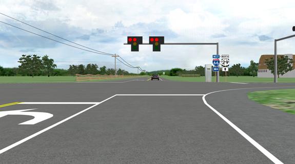
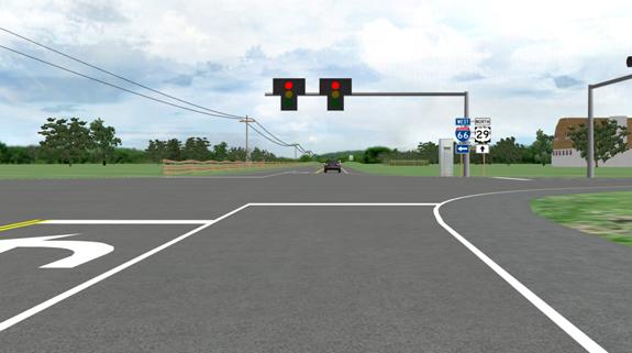
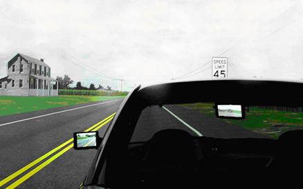
The distance between the participant's vehicle and the other vehicle was manipulated so that the average bumper-to-bumper space was approximately 1.2 s. An algorithm computed the difference between actual separation distance and the desired 1.2 s, and it adjusted the speed of the other vehicle to gradually reduce that difference. This algorithm worked well when participants maintained speeds close to the instructed cruise speed of 45 mi/h (72 km/h). Participants were encouraged to maintain the 45-mi/h (72-km/h) posted speed rather than adjust their speed to achieve a more comfortable separation distance.

Infrastructure-Based Warning

The infrastructure-based red light violator warning consisted of an immediate change from a green signal indication to red with no intervening amber interval. In addition to the red signal indications, red lights on both sides of the standard red light flashed alternately at 2 Hz. The infrastructure-based warning is depicted in figure 1. Figure 2 illustrates the normal (nonwarning) appearance of the red indication.

Figure 1. Screenshot. Simulated signalized intersection with activated infrastructure-based red light violator warning.

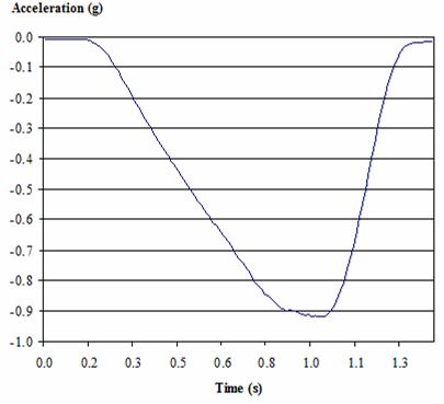
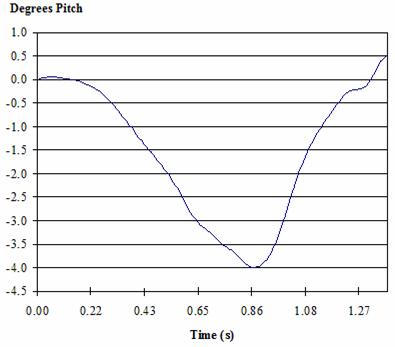
Figure 2. Screenshot. Simulated signalized intersection in normal operation.

In-Vehicle Warning

The in-vehicle warning consisted of the illumination of a red light-emitting diode (LED) icon on the vehicle's dashboard, a digitized voice message saying "danger, red light violator," and a brake pulse. The traffic signal remained green. The brake pulse was a deceleration of the vehicle slightly longer than 0.9 s that peaked at about -0.9 g (-29 ft/s² (8.8 m/s²)). The profile of the brake pulse deceleration is depicted in figure 3 with the initiation of the voice message as the reference point for the brake pulse. Because the driving simulator had no longitudinal movement, the main indication of braking was a sudden pitch forward that accompanied the visual indications of slowing. The pitch, measured from the driver's seat position, is shown in figure 4. The duration of the voice message was 1.3 s.

Figure 3. Graph. Brake pulse acceleration as a function of time shown relative to the onset of the voice message and red LED on dashboard.

Figure 4. Graph. Degrees of pitch in simulator cab as a function of time during in-vehicle emergency warning event given no driver input.

Combined Infrastructure-Based and In-Vehicle Warning

The combined infrastructure-based and in-vehicle warning was the simultaneous onset of the traffic signal mast arm warning and the in-vehicle warning.

Participants

Participants were recruited from the FHWA Human Centered Systems Participant Database. The database includes drivers from the District of Columbia metropolitan area who have responded to newspaper advertisements, internet postings, or word-of-mouth recruiting efforts. Participants included individuals who had participated in previous FHWA studies as well as newly recruited persons. Individuals who participated in the earlier red light violator warning studies were not recruited for this experiment. A total of 242 individuals were recruited. Of those, 46 failed to complete the study because of simulator-induced discomfort. Data from five participants were lost because of computer malfunctions. Thus, usable data were obtained from 191 participants. The age group and gender of these participants is summarized in table 1.

Table 1. Number of participants who completed the study.

The mean age of the under 65 years old group was 35 years (SD = 12.6), and the mean age of the 65 years old or older group was 72.3 years (SD = 9.1). All participants were licensed drivers, and a Snellen eye chart was used to verify that their corrected visual acuity was 20/40 or better in at least one eye.

Assignment to conditions was random but subject to the constraint that roughly equal proportions of participants of each gender and age grouping were assigned to each experimental condition.

Research Design

The experiment consisted of three warning types and four car-following conditions with 16 participants in each cell. The design is depicted in table 2. Although the intent was to have 16 observations within each combination of warning type and car-following condition, an error in the data collection routine resulted in the loss of data from one participant.

Table 2. Participants classified by warning type and car-following condition.

Protocol

Upon arriving at the research center, participants were asked to read and sign an informed consent form, after which, their visual acuity was assessed. A brief health screen questionnaire was administered to ensure that participants were in their usual state of health and that they were not impaired by drugs or alcohol. Participants were then escorted to the driving simulator where two tests purported to be sensitive to the effects of simulator sickness were administered—the Simulator Sickness Questionnaire (SSQ) and a sway magnetometry test of postural stability.^(6,7) These tests were administered before the participants entered the simulator to establish a baseline for later tests.

Participants were then seated in the driving simulator. The first of two simulation sessions was intended to allow participants to adapt to the vehicle's controls and performance. Participants were asked to accelerate, brake, and change lanes until they felt comfortable with the maneuvers. Once participants felt comfortable with the vehicle, the first drive was terminated, and participants were again administered the SSQ and a sway magnetometry test. Participants then returned to the driving simulator and began the experimental session.

Three similar sets of instructions were used. The specific instructions depended on the assigned car-following condition. The instructions to participants who followed another vehicle are shown below, and the italicized portion was tailored to this group.

You will be driving on a simulated two-lane rural road that is loosely based on U.S. 29 in Manassas, VA. On this road, you will encounter a signalized intersection about once per mile. The signal will change—first to yellow, then to red—and you will need to decide whether to proceed through the intersection or to stop to avoid running a red light. You should make this decision the same way you would when driving your own vehicle in the real world. In other words, drive as you normally would.

Be aware that the posted speed will always be 45 mph. You may be reminded to "watch your speed" if you drive too much differently from the posted speed.

We are interested in how people's decisions at traffic signals are affected by whether other vehicles are around. In this simulation, you may find that no other cars are on the road or that there is a car in front of or behind you. Check your rear view mirrors as you normally would.

Regardless of whether there are cars in front of or behind you, you should try to maintain 45 mph except when you need to respond to traffic signals. Leading vehicles are programmed not to exceed 45 mph. If you accelerate too quickly, you may end up having to brake to avoid hitting the vehicle ahead. On the other hand, if you accelerate very slowly, the lead vehicle will slow down, and you may still find yourself closing quickly on it. Therefore, try to accelerate at a moderate rate and then maintain 45 mph. The vehicle ahead will adjust its speed so that when you reach the next intersection, you will be close behind it. In this case, we are interested in how you respond to a traffic signal when there is a vehicle close ahead.

Your simulated vehicle is equipped with an experimental warning system that is being tested in several States. This device communicates with the intersection traffic signals to determine the state of the signal and whether someone is about to run the red signal. The box on the dashboard has a blue indicator that comes on whenever the vehicle is approaching an intersection that is equipped to provide your car this information. If the experimental system spots a red light violator, the indicator light turns red. In addition, the car may brake sharply for a half-second, and a voice message may come on that says "Danger, red light violator." If this warning should come on, respond appropriately.

The tailored portion of the instructions was intended to encourage participants to accept the relatively short following distance.

Participants then drove down a simulated rural road that had a signalized intersection every 0.5 mi (0.8 km). At most of the signalized intersections, an amber signal was triggered at some point as the driver approached. The change from a green to an amber interval was manipulated so that participants stopped at half of the intersections and did not stop at the other half. The purpose of this manipulation was to enable the computation of the mean time-to-stop line (TTSL) at which the participant decided whether to stop for the traffic signal.

After the average TTSL was computed, the red light violator warning was given at a subsequent intersection. The warning was triggered at a TTSL substantially less than the average TTSL.

The Driving Simulation

FHWA's HDS is a relatively high-fidelity research simulator. Simulator components include a 1998 Saturn SL1 chassis, five projectors, and a cylindrical projector screen. Each projector has a resolution of 2,048 pixels horizontally and 1,536 pixels vertically. The image on the screen wraps 240 degrees around the forward view. Measured horizontally, the projection screen is 9 ft (2.7 m) from the driver's design eye point. Under the vehicle chassis, there is a 3 degree-of-freedom (roll, pitch, and heave) motion system. A sound system provides engine, wind, tire, and other environmental sounds. The vehicle dynamics model is calibrated to approximate the characteristics of a small passenger sedan, and data capture is synchronized to the frame rate of the graphics cards (mean = 100 frames per second). Data recorded from the vehicle dynamics model includes speed, longitudinal acceleration, lateral acceleration, accelerator pedal displacement, brake pedal displacement, vehicle position, and heading.

To enable the simulation of a vehicle closely following the participant's vehicle, rear view mirrors were simulated using 7.8-inch (19.7-cm)-wide by 4.8-inch (12-cm)-high color liquid crystal displays (LCD) with 800 pixels horizontally and 480 pixels vertically. These displays had a wide viewing angle (140 degrees horizontally and 100 degrees vertically and a maximum contrast ratio of 400:1). Left and right outside simulated mirrors were mounted over the Saturn's original outside mirrors. The center-mounted rear view LCD was placed as near as possible to the location of the vehicle's original mirror. The left outside and center-mounted mirror displays are shown in figure 5.

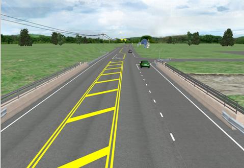
Figure 5. Screenshot. Left outside and center-mounted rear view mirrors viewed from behind the vehicle.

In the condition in which another vehicle followed the participant's vehicle, the retinal angle subtended by the following vehicle image was calibrated to appear in the simulated mirror at the correct size for a reflected image from the simulated following distance. Despite the careful calibration of the image size, informal questioning suggested that most participants perceived that the distance was less than 1.2 s.

The simulated environment was a two-lane rural highway. At every 0.5 mi (0.8 km), a signalized intersection was encountered. At each intersection, the road widened to three lanes with the added lane dedicated to left turns. Cultural features such as barns, grain elevators, and farm houses varied somewhat from intersection to intersection, but the roadway alignment was always the same. About 455 ft (139 m) upstream of the signalized intersection, a stop-controlled road joined from the right forming a T-intersection. A right-turn deceleration lane preceded that intersection.

Buildings or mounds at each signalized intersection prevented participants from seeing approaching traffic on the intersecting roadway. These visual obstructions were present to discourage participants from making stop or go decisions based on the presence or absence of conflicting traffic.

Each encounter with an intersection at which the signal changed comprised a trial. In the conditions that included either a preceding or following vehicle, the other vehicle turned off onto the T-intersecting side-road every fourth to sixth intersection. When the other vehicle turned off, another vehicle turned onto the main road either ahead of or behind the participant, as was appropriate to the assigned car-following condition. Whenever the lead or following vehicles changed, the subsequent traffic signal remained green. In the condition in which there was no other vehicle, green signals were shown at the same frequency as in the leading or following conditions. Figure 6 shows a leading vehicle turning right and the vehicle that replaced it.

Figure 6. Screenshot. Other car leads condition.

At all other intersections, an amber change interval occurred at some point on the approach. The first amber change interval began when the participant's TTSL was 0.5 s. If the participant did not stop (which was always the case at this distance), the TTSL was increased by 0.5 s on each subsequent trial until the participant stopped. After a stop, the TTSL was decreased by 0.4 s on each subsequent trial until the participant proceeded without stopping. The TTSL was then increased by 0.3 s on each trial until the participant stopped. The TTSL was then decreased by 0.2 s on each trial until the participant once again proceeded through the intersection without stopping. The process of increasing and decreasing the TTSL by 0.2 s continued until the participant had switched between stop and go decisions 10 times. The last eight TTSLs for which a switch in decision occurred were then averaged, and this mean was used as the participant's decision point. The SD of these last eight TTSLs was also computed.

The red light violator warning was triggered on the next trial. The TTSL of the warning was determined by the following equation:

TTSl_W = decision point - (1.3 x SD)

Figure 7. Equation. Calculation for the TTSL_W.

The SD was multiplied by 1.3 because under a normal distribution, slightly more than 90 percent of the area falls below 1.3 SDs above the mean. Thus, assuming that the sample of decision points came from a normal distribution, the TTSL for the collision warning, TTSL_W, would yield a probability of less then 10 percent that the participant would have stopped for an amber change interval at that TTSL. Thus, following the warning, if more than 10 percent of participants are delayed by at least 1 s in reaching the stop line, the level of responding could be attributed to the warning.

Table 3 shows the results from the modified method of limits procedure for one participant. The column labeled "Score" shows the TTSL for trials on which the driver's behavior changed from the previous trial. The last eight scores, which are bolded and italicized in the table, were used in calculating TTSL_W.

Table 3. Modified method of limits results from one participant.

Note: Blank cells indicate that there was no change from the behavior on the previous trial. The bold and italicized text indicates that those scores were used in calculating the TTSL_W.

Results

Although the main focus of the research was to evaluate collision warnings, the findings regarding the amber change interval responses are presented first because the timing of the warnings was dependent on them. The amber change interval findings may be of interest because they provide information concerning individual driver differences in decisionmaking at traffic signals.

The amber signal response portion of the results includes the following:

• The number of trials required to obtain the TTSL_W.
• The TTSL frequency distribution.
• The mean speeds and SD in speeds at the onset of the amber change interval.
• Accelerator release response times to the onset of the amber signal.
• Brake pedal response times to the onset of the amber signal.
• Peak decelerations in response to the amber signal onset.

The warning response portion of the results includes the following:

• The distribution of warning onset times.
• The success in delaying arrival at the stop line as a function of warning type.
• Accelerator release response time as a function of warning type.
• Brake press response time as a function of warning type.
• Peak decelerations in response to warning onset.

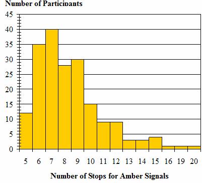
Amber Signal Responses

The method of limits was used to calculate an appropriate TTSL_W. However, the amber change interval responses that resulted are of interest in their own right because they allow for the examination of individual differences in dilemma zone and option zone attributes.⁽⁸⁾ Because the only times scored were from trials when participants changed their response relative to the previous trial (i.e., from stop to go, or go to stop), the total number of trials varied between participants. Figure 8 shows the frequency distribution for the number of stop decisions required before participants reached the criterion of 10 changes in response. Only 12 participants required the minimum number of stops, which was 5. The modal number of stops to reach the criterion was 7 (40 participants). One participant stopped 20 times before reaching the criterion.

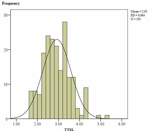
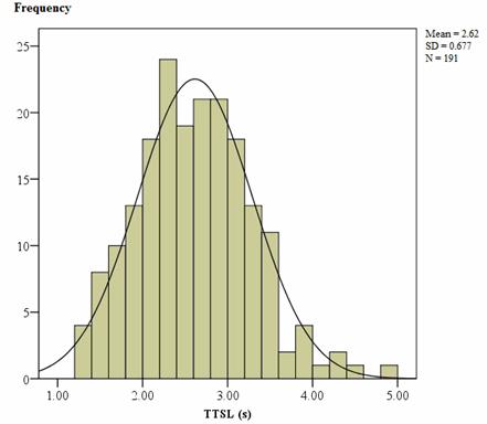
Figure 8. Graph. Frequency distribution of the number of stops required by participants to complete the modified method of limits procedure.

The frequency distribution of mean decision points of the 191 participants is shown in figure 9. The bell curve represents normal distribution, with the observed mean of 2.92 and observed SD of 0.664.

Figure 9. Graph. Distribution of the means for the TTSL decision points.

A multivariate analysis of variance was performed with mean speeds and SDs of the mean speeds of individual participants as dependent measures and age group and car-following conditions as independent measures. Because the two conditions in which the participants followed another vehicle (lead vehicle stops and lead vehicle goes) were only different from each other on the final (warning) trial, those groups were combined in this analysis. The multivariate effects of age group and following condition were significant by Wilks' lambda, both p < 0.01. Post hoc tests showed that the older adults drove more slowly than the younger adults, F (1, 105) = 15.3, p < 0.01. Also, there was difference between participant speed variability in the car-following condition in which participants followed another vehicle than in the other car-following conditions, F (2, 185) = 8.6, p < 0.001. The mean approach speed of the younger drivers was 49.5 mi/h 7 (9.7 km/h) with a standard error of 0.5 mi/h (0.8 km/h). The speed variability effect is shown in figure 10 in which error bars represent the 95-percent confidence limits for the means. Overall, these findings suggest that the instruction to maintain the posted speed of 45 mi/h (72 km/h) was observed. However, on average, older drivers drove slightly slower than younger drivers. The presence of a leading vehicle caused more variation in speed but did not significantly affect the mean speed of either age group.

Figure 10. Graph. Mean within participant variability in speed as a function of car-following conditions.

In the above analyses, the two conditions in which the participant followed another vehicle were treated as a single condition because these treatments did not differ on amber change interval trials. In addition, the type of warning to be given was not considered for the same reason. However, as a check on the effectiveness of random assignment of participants to conditions, the mean TTSL_W was tested as a function of the four car-following conditions and three warning conditions.

Unexpectedly, an interaction between warning type and car-following condition was obtained, F (6, 167) = 2.3, p < 0.05. As can be seen in figure 11, the mean TTSL of the participants in the infrastructure-based warning group who followed a lead vehicle that would stop after the warning was initiated had a mean TTSL of 0.6 s more than that of any of the other 11 groups. This effect was not the result of outliers—the entire distribution for this group was shifted. The interaction may have been the result of differences in mean speed on the approach to the intersection. When speed was entered as a covariate in the multivariate analysis, the interaction was no longer significant. The linear correlation (r = 0.252) between speed and TTSL was significant, p < 0.001.

Figure 11. Graph. Mean TTSL for amber signal decision as a function of assignment to warning and car-following conditions.

Response Time

Two response times were calculated for the amber change interval trials: (1) accelerator release latency and (2) brake press latency. Only trials were included in which the participants were depressing the accelerator and not the brake pedal when the signal changed. Because six individuals either drove with a foot on each pedal or always released the accelerator when nearing intersections, they were excluded from the response time analysis. For each of the remaining participants, two mean latencies were computed from all trials that ended in a stop and allowed both an accelerator release and a brake depression response time to be recorded. For the purpose of this analysis, because not all drivers come to a complete stop, a stop is defined as a delay of reaching the stop line 1 s or more that is not associated with a red light violation. Accelerator release latency is computed as the time between the onset of the amber signal and the end of accelerator pedal depression. Brake depression latency is computed as the time between the onset of the amber signal and the beginning of brake pedal deflection. For each participant, mean accelerator release and brake press latencies were computed by averaging across stops. The means of the accelerator release and mean of brake depression latency means are shown as a function of car-following condition in figure 12.

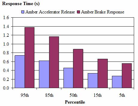
Figure 12. Graph. Mean of average accelerator release and brake response latencies as a function of car-following conditions.

A multivariate analysis of variance was performed with the two response latencies as the dependent variable and the three levels of car-following conditions as the independent variable. A significant car-following effect was obtained, F (4, 362) = 2.6, p < 0.05. As can be seen in figure 12, the response latencies of participants in conditions that followed another vehicle were longer on average than the latencies of the other participants. Error bars in the figures represent the 95-percent confidence limits for the means.

The distributions of mean accelerator release and brake press response latencies are shown in figure 13 and figure 14. As is typical of response time distributions, these distributions were somewhat positively skewed. It is frequently assumed that response times follow a lognormal distribution.^(9,10) The Traffic Engineers Handbook states that 1 s is typically used as the driver brake reaction time when computing the length of amber change intervals.⁽¹¹⁾ Figure 15, which shows the 95th-, 85th-, 50th-, 15th-, and 5th-percentile acceleration release and brake press latencies estimated using a lognormal transformation of the observed data, suggests that 1 s may be a reasonable estimate for the 50th-percentile driver, but it would not be sufficient for 85th- or 95th-percentile drivers.⁽¹⁰⁾ The estimated and observed values for the 50th-percentile (median) response time are always equal when this transformation is used.

Figure 13. Graph. Accelerator amber onset response latency distribution.

Figure 14. Graph. Brake amber onset response latency distribution.

Figure 15. Graph. Estimated population percentiles for accelerator and brake response times calculated using a lognormal transformation.

Peak Deceleration

The mean TTSL at which the amber signal was triggered was 3 s, and the median brake response time was 0.88 s. Thus, on average, participants had 2.12 s to decelerate to a stop at the stop line. At 50 mi/h (80 km/h), which was about the average approach speed of the younger participants, an average deceleration rate of 0.24 g (7.73 ft/s² (2.36 m/s²)) would be required. The maximum deceleration for each stop was measured. The mean maximum deceleration was 0.9 g (29 ft/s² (8.8 m/s²)), which was far more than was required and than the real world comfortable deceleration of 0.27 g (8.6 ft/s² (2.6 m/s²)) suggested by Wilson, Moyer, and Barnett; the 0.46 g (14.8 ft/s² (4.5 m/s²)) suggested by Durth and Bernhard; or the 0.34 g (11 ft/s² (3.4 m/s²)) reported by Wortman and Matthias.^(12-14) However, the high deceleration force observed in the driving simulator may have been a result of difficulty in judging rate of deceleration perhaps because of the lack of longitudinal jerk or movement in the simulator.

Typical stopping behavior began with hard braking that slowed the vehicle to approximately 5 mi/h (8 km/h) 50 ft (15 m) from the stop line, at which point the brake pedal was released, and the vehicle coasted toward the stop line. According to Boer et al., patterns of braking like this are common among novice simulator drivers.⁽¹⁵⁾ They attribute this braking phenomenon to differences in proprioceptive and vestibular acceleration cues combined with distance and speed cue distortions that are present in varying degrees in all driving simulators.

Warning Responses

Warning Onset

The frequency distribution for TTSL_W is shown in figure 16.

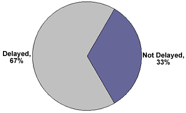
Figure 16. Graph. Distribution of TTSL for initiating the warning.

Warning Effectiveness

The success of the warnings in delaying arrivals at the stop line is shown in table 4 as a function of warning type and car-following condition. A logit model was used to evaluate the effects of warning and car-following as well as their interaction. A logit analysis was used because the independent variables (car-following condition and warning type) were classification variables, and the dependent variable (delay success) was binary. Although logit analysis is similar to the more familiar analysis of variance in that it includes both main effects and interactions, it differs in how statistical significance is evaluated—rather than providing statistical significance for each effect, the model as a whole is evaluated, and the effects are dropped from the model until the model no longer accounts for the observed variability. In a logit analysis, the best fitting model is the most economical model for which the goodness-of-fit does not differ significantly from the full model.^(16,17)

Table 4. Failure and success in delaying arrival at the stop line by 1 s as a function of warning type and car-following condition.

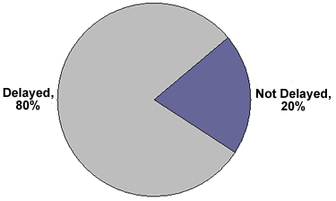
The car-following condition had no statistically significant effect on the model's goodness of fit. That is, eliminating the car-following independent variable and the interaction of car following with warning resulted in a model that adequately fit the delay results, (9) = 7.1, p > 0.63. Elimination of warning from the model yielded a significant lack of fit, (8) = 25.5, p < 0.001. The results with only the significant independent variable, warning, are shown in figure 17 through figure 19.

Figure 17. Graph. Percentage of drivers delayed by a least 1 s in arrival at an intersection after the onset of an infrastructure-based warning.

Figure 18. Graph. Percentage of drivers delayed by a least 1 s in arrival at an intersection after the onset of an in-vehicle warning.

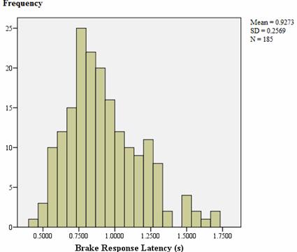
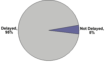
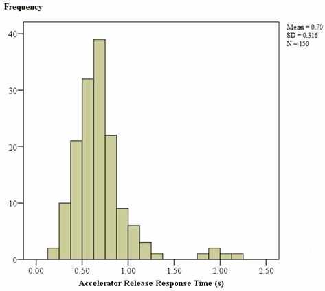
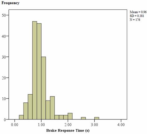
Figure 19. Graph. Percentage of drivers delayed by a least 1 s in arrival at an intersection after the onset of simultaneous infrastructure-based and in-vehicle warnings.

Subsequent analyses showed that the infrastructure-based and in-vehicle groups did not differ significantly from each other in frequency of delay, (1) = 2.7, p > 0.05. The group that received the simultaneous infrastructure-based and in-vehicle warnings was delayed significantly more than the in-vehicle group, (1) = 7.1, p < 0.01. It should be noted that even the least effective warning, the infrastructure-based only warning, delayed significantly more than the approximately 10 percent of drivers that would have been expected to stop in response to the onset of an amber interval, (1) = 224.8, p < 0.001.

Warning Response Time

Two measures of response time to the warning were available: (1) response latency from the onset of the warning to complete release of the accelerator pedal and (2) latency from the onset of the warning to the initiation of the brake press. The former required that the accelerator was depressed when the warning was initiated. The latter required that the brake was not already depressed when the warning came on.

Figure 20 shows the overall distribution of accelerator release response times (n = 150), and figure 21 shows the overall distribution of brake pedal response times (n = 176). Although the response time distributions were slightly skewed, the skew was not deemed severe enough to warrant transformation of the data before conducting further analyses.

Figure 20. Graph. Accelerator release response times following the onset of warning.

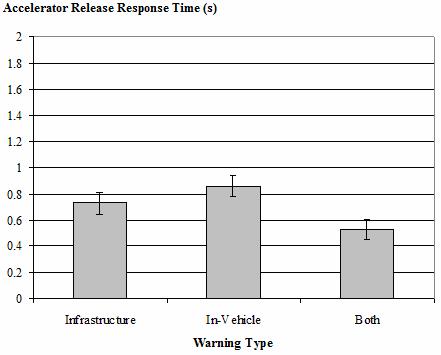
Figure 21. Graph. Brake press response times following the onset of warning.

The data from the 141 participants who had both accelerator release and brake press response times were submitted to multivariate analysis of variance. The two response times were used as dependent measures, and warning type and car-following conditions were used as independent variables. Only the effect of warning type was statistically reliable by Wilks' lambda, F (4, 256) = 10.7, p < 0.001.

Mean accelerator release latencies for all 150 participants who released the pedal following the onset of the warning are shown in figure 22. Error bars in the figure represent the 95-percent confidence intervals of the means. The shortest mean accelerator release latency was 0.53 s to the simultaneous in-vehicle and infrastructure-based warnings. The mean response to the simultaneous warnings was significantly shorter than the 0.73-s mean response to the infrastructure-based only warning, which itself was significantly shorter than the 0.86-s response to the in-vehicle only warning.

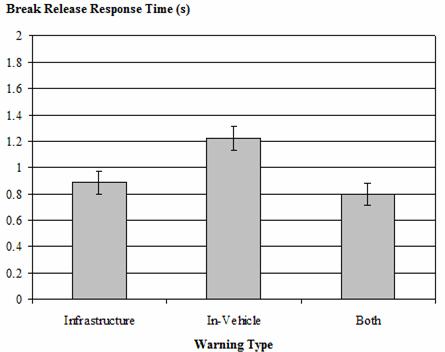
Figure 22. Graph. Mean accelerator release latency as a function of warning type.

Mean brake press response times are shown in figure 23 as a function of warning type. The simultaneous infrastructure-based and in-vehicle warnings resulted in a mean brake response latency of 0.80 s, which was significantly less than the 0.89-s mean latency following the onset of the infrastructure-based only warning. The longest brake response latency, 1.22 s, was to the in-vehicle only warning, which was significantly slower than the response to the infrastructure-based only warning.

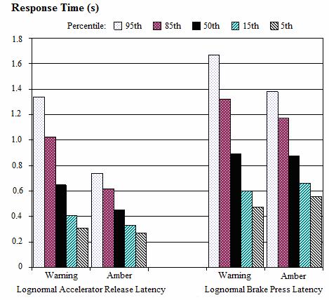
Figure 23. Graph. Mean brake press latency as a function of warning type.

Amber change interval responses to the warnings were subjected to a lognormal transformation, and estimates of the 95th-, 85th-, 50th-, 15th-, and 5th-percentile response times were computed. These estimates are shown in figure 24. For comparison, the estimates for amber change interval that were presented in figure 15 are shown alongside the warning response estimates. The 95th- and 85th- percentile latencies to the warning were longer than the latencies to the amber change interval, reflecting a surprise factor that was not present for the amber change interval. According to Olson and Sivak, responses to unexpected stimuli are typically longer than for expected stimuli.⁽¹⁸⁾

Figure 24. Graph. Lognormal estimates of the population response times for accelerator release and brake press.

Peak Deceleration

For each warning event, which spanned the time from the onset of the warning until participants either came to a stop or crossed the stop line, the peak rate of deceleration was recorded for all participants who were delayed by at least 1 s in reaching the stop line. The mean was the same across treatment groups and approximated the maximum deceleration rate possible with the vehicle dynamic model used for the simulation: 0.969 g (31.2 ft/s² (9.5 m/s²)). Thus, peak deceleration was the same for the amber change interval as it was for the warnings.

Discussion

As stated previously, the objectives of the study were as follows:

• To evaluate three warnings that could be given to potential victims of red light violators.
• To determine whether responses to these warnings would be influenced by the presence other vehicles.
• To characterize driver decisionmaking when approaching a traffic signal that changes from green to amber (amber change interval onset).

This discussion relates the previously stated results to each of these objectives. The last objective will be discussed first, as the results of the drivers' reactions to the amber change interval were used to determine when the warning would be initiated.

Driver DecisionMaking at Onset of the Amber Change Interval

The motivation for measuring drivers' responses to amber signal onset was the finding in an earlier FHWA study in which drivers were delayed by the onset of an amber signal 31 percent of the time even when the change came at a distance from the stop line where other data suggested that no drivers would stop.^(19,5) This led to problems in interpreting the finding that approximately 64 percent of drivers stopped for a warning that was initiated at that distance to the stop line. It became evident that the effectiveness of intersection collision warnings had to be evaluated in relation to amber change interval responses. Because the distance at which the decision to stop following the onset of the amber appeared to vary across drivers, a procedure that allowed tailoring of the warning onset distance to individuals was needed.

The present study was designed so that drivers would be unlikely to be delayed by an amber change interval at the TTSL at which the warning was given. To that end, a modified method of limits was used to identify the decision point of individual drivers.

The mean TTSL decision point did not vary as a function of the presence of other vehicles either ahead of or following the participant vehicle. However, mean response times to accelerator release and brake press were longer when there was a vehicle ahead of the participant. There was also greater variability in vehicle speed when drivers were following another vehicle. It is interesting to note that although reaction time was slightly slower and speed was more variable when following another vehicle—perhaps because the leading vehicle was somewhat distracting—the decision point was not significantly affected by other vehicles.

The method of limits procedure enabled relatively quick convergence on a mean decision point that was likely to be highly reliable because it was based on repeated observations that bracketed the variations in individual responses. The estimates of response times that were obtained tended to be faster than those typically reported in the literature, but this may be explained by the unique circumstances underlying the use of the method of limits. For instance, Wortman and Matthias reported a mean brake response time of 1.3 s at selected intersections in Arizona compared to the mean across conditions of 0.93 s found in this study.⁽²⁰⁾ However, Wortman and Matthias were recording the onset of brake lights of the first vehicle to stop following the onset of the amber. The onset of the amber in their case was not necessarily as near the driver's decision point as it was in the present study. In their study, the mean distance from stop line was 247 ft (77 m) at the onset of the amber, whereas in this study, the mean distance at onset was 208 ft (63.4 m). It was reasonable to expect that response times were shorter as the available stopping distance decreased. In fact, this is what Inman et al. reported in their analysis of brake response times to amber onset in a test-track environment.⁽⁵⁾ Their data suggested a 0.3-0.5-s difference in response time with a 75-ft (22.9-m) change in distance from the stop line. Another factor that could have led to a decrease in response time in the present study relative to other studies was the anticipation of the driver. In the present study, the amber change interval occurred at about 83 percent of the intersections. Participants were likely to discover early on that the only change from trial-to-trial was when or if the signal would change, although the traffic signal change was not part of the instructions.

The peak deceleration rates in stopping for the amber change interval did not reflect real- world rates. Typical deceleration rates used to determine amber change interval lengths ranged from 0.27 to 0.47 g.^(21,22) The mean maximum deceleration rate in this study was 0.9 g, which was well outside the real-world range and thus should not be used for extrapolating to the real world. However, the required average deceleration, given the observed mean reaction time and distance to the stop line, was 0.24 g, which was well within the real-world deceleration rates. The maximum deceleration observed in the simulator was likely due to participants' difficulty in judging their rate of deceleration because of the lack of appropriate proprioceptive and vestibular feedback.

Warning Effectiveness

In previous FWHA experiments, the red light violator warning was given when participants were at a fixed distance from the stop line. When the warning was given at 185 ft (56.4 m) and the participants were traveling at approximately 45 mi/h (72 km/h), 64 percent of participants were delayed by 1 s or more in the driving simulator, and 90 percent of participants were delayed by that amount in a test on a closed road. In the present study, TTSL was used instead of distance, and the TTSL varied widely across participants. What all participants had in common was that the warning was given at a point when they were unlikely to have stopped for an amber change interval. The average distance from the intersection was 172 ft (52.4 m) from the stop line, which was 13 ft (3.9 m) closer on average than in the previous studies. However, the percent of participants delayed by the warnings was greater than in the earlier studies. This was probably the result of adjusting the TTSL for the warning to be relative to the mean TTSL of each individual's responses to the amber change interval. For five participants who routinely entered the intersection more than 4 s after the onset of the amber change interval and thus routinely violated the red light, the adjustment also resulted in the presentation of the red light violation warning when they were more than 4 s from the stop line. All three warnings were far more effective in delaying participants than an amber change interval.

The previous studies evaluated only infrastructure-based warnings. However, the U.S. Department of Transportation's Cooperative Intersection Collision Avoidance (CICAS) program has placed an emphasis on in-vehicle or driver-vehicle interface warnings.⁽²³⁾ Therefore, the present study evaluated both infrastructure-based and in-vehicle warnings. Because infrastructure-based and in-vehicle warnings were not necessarily mutually exclusive, the combination of the two warnings was also evaluated.

The results with the infrastructure-based warning were similar to those obtained in the previous simulator study-67 percent of participants were delayed in the present study versus 64 percent of participants who were delayed in the two most comparable conditions in the previous study. The difference between the infrastructure-based and in-vehicle warnings was not statistically significant. The major new finding was that when the two warnings were combined, the effect was additive so that 95 percent of participants in the combined warning condition were delayed. The finding suggests that infrastructure-based and in-vehicle warnings alone can be effective and that the investment in one warning type should not preclude investment in the other. Either warning type has the potential to markedly enhance the effectiveness of the other.

Response times were shorter to the infrastructure-based warning than to the in-vehicle warning. This may indicate that the infrastructure-based warning was more compatible with the driving task than the in-vehicle warning. The infrastructure-based warning had two advantages over an in-vehicle warning. First, it presented the warning in a region where the driver was expected to look. Second, it did not present conflicting information. The latter point is potentially important—when an in-vehicle collision warning is given alone, the traffic signal remains green and conflicts with the message coming from the vehicle. The delayed response to the in-vehicle warning may have been caused by this conflict.

Nonetheless, the in-vehicle warning was effective despite the delayed response. The brake pulse portion of the warning initiated braking before the drivers began to brake, thus partially compensating for the drivers' longer response times. In future systems, in-vehicle warnings that do not include a brake pulse or that have a weaker brake pulse than the one used in this study might not be as effective as the in-vehicle warning used in the present study.

The combined warnings reduced the response time by one-tenth of a second relative to the infrastructure-based warning. As with the delay criterion, the response time measure suggests that the combination of the infrastructure-based and in-vehicle warnings is most effective. The quicker the driver responds, the lower the rate of deceleration that is required. This effect should have safety implications such as increased vehicle control and decreased potential rear-end conflicts when compared to either in-vehicle or infrastructure-based warnings alone.

It is interesting to note that response times to the amber change interval were faster than to the warning. This suggests that participants were anticipating the amber change interval as they approached the intersection, but they were not anticipating a warning. The brake response time to the warnings about the same as the 50th-percentile "surprise" response time reported by Olson and Sivak.⁽¹⁸⁾

The presence of vehicles ahead of or behind participant vehicles had no significant effect on responses to the warnings or on the decision point for the amber phase change. Having a vehicle ahead did affect mean response time to the amber change interval, but it did not appear to affect the decision to stop.

Recommendations

The results of this study suggest that a combined infrastructure-based and in-vehicle warning could be highly effective in reducing crossing path crashes and fatalities at signalized intersections.

However, the findings also suggest that driver variability in response to both amber change intervals and collision warnings may pose a serious rear-end collision challenge. Some participants responded to warnings by delaying intersection entry by 1 s for a warning issued when their TTSL was only 1.5 s. Other participants were warned when their TTSL was more than 4 s. The study was not designed to test how the response time of lead vehicles affected the decision criteria or response time of following drivers, but this issue would certainly need to be addressed before a red light violator warning could be fielded.

The present results favor further research and development of a system to warning both red light violators and drivers at risk from red light violators. In the United States, the CICAS program is developing an in-vehicle warning.⁽²³⁾ In Europe, the SAFESPOT™ program is developing similar warning applications.⁽²⁴⁾ Although both programs are utilizing infrastructure to support communications to the vehicle, neither is currently proposing infrastructure-based driver interfaces to address straight crossing path crashes. The results of this study suggest that the effectiveness of these systems might be considerably enhanced by the addition of infrastructure-based warnings.

References

1. National Highway Traffic Safety Administration. (2007). Fatal Accident Reporting System. Obtained from: http://www-fars.nhtsa.dot.gov/QueryTool/QuerySection/SelectYear.aspx. Site last accessed June 1, 2009.
2. National Highway Traffic Safety Administration. (2009). National Automotive Sampling System General Estimates System. Obtained from: http://www.nhtsa.dot.gov/PEOPLE/ncsa/nass_ges.html. Site last accessed June 1, 2009.
3. Zimmerman, K. and Bonneson, J.A. (2005). "Investigation of Time into Red for Red Light-Related Crashes," Transportation Research Record, 21-28, Transportation Research Board, Washington, DC.
4. Ferlis, R.A. (2002). Analysis of an Infrastructure Collision Avoidance Concept for Straight Crossing Path Crashes at Signalized Intersections, 81st Annual Meeting of the Transportation Research Board, Washington, DC.
5. Inman, V.W., Davis, G.W., El-Shawarby, I., and Rakha, H. (2008). Test Track and Driving Simulator Evaluations of Warnings to Prevent Right-Angle Crashes at Signalized Intersections, FHWA-HRT-08-070, Federal Highway Administration, McLean, VA.
6. Kennedy, R.S., Lane, N.E., Berbaum, K.S., and Lilienthal, M.G. (1993). "Simulator Sickness Questionnaire: An Enhanced Method for Quantifying Simulator Sickness," The International Journal of Aviation Psychology, 3, 203-220.
7. Cobb, S.V. and Nichols, S.C. (1998). "Static Posture Tests for the Assessment of Postural Instability After Virtual Environment Use," Brain Res Bull JT—Brain Research Bulletin, 47, 459-464.
8. Yan, X., Radwan, E., Klee, H., and Guo, D. (2005). "Driver Behavior During Yellow Change Interval," Driving Simulation Conference, 88-97, Orlando, FL.
9. Setti, J.R., Rakha, H., and El-Shawarby, I. (2007). Analysis of Brake Perception-Reaction Times on High-Speed Signalized Intersection Approaches, 86th Annual Meeting of the Transportation Research Board, Washington, DC.
10. Taoka, G.T. (1989). "An Analytical Model for Driver Response," Transportation Research Record 1213, 1-5, Transportation Research Board, Washington, DC.
11. Institute of Transportation Engineers. (2009). Institute of Transportation Engineers Traffic Engineering Handbook, 6th ed., Washington, DC.
12. Wilson, E.E., Moyer, R.A., and Barnett, J. (1941). Deceleration Distances for High Speed Vehicles, Highway Research Board Annual Meeting, Washington, DC.
13. Durth, W. and Bernhard, M. (2000). Revised Design Parameters of Stopping Sight Distance, 2nd International Symposium on Highway Geometric Design, German Institute for Normalization, Mainz, Germany.
14. Wortman, R.H. and Matthias, J.L. (1983). An Evaluation of Driver Behavior at Signalized Intersections, Arizona Department of Transportation, Phoenix, AZ.
15. Boer, E.R., Kuge, N., and Yamamura, T. (2001). Affording Realistic Stopping Behavior: A Cardinal Challenge for Driving Simulators, Inrets, Driving Simulation Conference Europe, Sophia Antipolis, France.
16. Garson, D.G. (2006). Logit, Probit, and Log-linear Models, PA 765. Obtained from: http://faculty.chass.ncsu.edu/garson/PA765/logit.htm. Site last accessed August 23, 2006.
17. Tabachnik, B.G. and Fidell, L.S. (1996). Using Multivariate Statistics, HarperCollins Publishers, New York, NY.
18. Olson, P.L. and Sivak, M. (1986). "Perception-Response Time to Unexpected Roadway Hazards," Human Factors, 28, 91-96.
19. Inman, V.W., Davis, G.W., El-Shawarby, I., and Rakha, H. (2006). Field and Driving Simulator Validations of System for Warning Potential Victims of Red-Field and Driving Simulator Validations of System for Warning Potential Victims of Red light Violators, 85th Annual Meeting of the Transportation Research Board, Washington, DC.
20. Wortman, R.H. and Matthias, J.S. (1983). "Evaluation of Driver Behavior at Signalized Intersections," Transportation Research Record, 10-20, Transportation Research Board, Washington, DC.
21. ITE Technical Committee 4TF-1. (1994). "Determining Vehicle Signal Change and Clearance Intervals," Compendium of Technical Papers, 64th ITE Annual Meeting, Dallas, TX.
22. Garber, N.J. and Hoel, L.A. (2009). Traffic and Highway Engineering, 4th ed., Cengage Learning, Toronto, Canada.
23. Research and Innovative Technology Administration. (2004). CICAS Workshop Report. Obtained from: http://www.its.dot.gov/cicas/cicas_workshop.htm. Site last accessed July 21, 2009.
24. European Commission Information Society and Media SAFESPOT Integrated Project. (2009). SAFESPOT Integrated Project. Obtained from: http://www.safespot-eu.org. Site last accessed July 21, 2009.