U.S. Department of Transportation
Federal Highway Administration
1200 New Jersey Avenue, SE
Washington, DC 20590
202-366-4000
Federal Highway Administration Research and Technology
Coordinating, Developing, and Delivering Highway Transportation Innovations
| REPORT |
| This magazine is an archived publication and may contain dated technical, contact, and link information |
|
| Publication Number: FHWA-HRT-15-048 Date: June 2015 |
Publication Number: FHWA-HRT-15-048 Date: June 2015 |
The EB methodology for observational before-after studies was used for the evaluation.(6) This methodology is considered rigorous in that it accounts for regression-to-the-mean using a reference group of similar but untreated sites. In the process, SPFs are used for the following reasons:
The methodology also provides a foundation for developing guidelines for estimating the likely safety consequences of a contemplated strategy.
In the EB approach, the change in safety for a given crash type at a site is given in figure 1:

Figure 1. Equation. Estimated change in safety.
Where:
λ = expected number of crashes that would have occurred in the after period without the strategy.
π = number of reported crashes in the after period.
In estimating λ In the EB procedure, the SPF is used to first estimate the number of crashes that would be expected in each year of the before period at locations with traffic volumes and other characteristics similar to the one being analyzed (i.e., reference sites). Annual SPF multipliers were calibrated to account for temporal effects on safety (e.g., variation in weather, demography, and crash reporting).
In the EB procedure, the SPF is used to first estimate the number of crashes that would be expected in each year of the before period at locations with traffic volumes and other characteristics similar to the one being analyzed (i.e., reference sites). The sum of these annual SPF estimates (P) is then combined with the count of crashes (x) in the before period at a strategy site to obtain an estimate of the expected number of crashes (m) before strategy. This estimate of m is seen in figure 2:

Figure 2. Equation. EB estimate of expected crashes.
W is estimated from the mean and variance of the SPF estimate as seen in figure 3:

Figure 3. Equation. EB weight.
Where:
k = constant for a given model and is estimated from the SPF calibration process with the use of a maximum likelihood procedure. In that process, a negative binomial distributed error structure is assumed, with k being the overdispersion parameter of this distribution.
A factor is then applied to m to account for the length of the after period and differences in traffic volumes between the before and after periods. This factor is the sum of the annual SPF predictions for the after period divided by P, the sum of these predictions for the before period. The result, after applying this factor, is an estimate of the variance of λ.
The estimate of λ then summed over all sites in a strategy group of interest (to obtain λsum) and compared with the count of crashes observed during the after period in that group (πsum). The variance λ of is also summed over all sites in the strategy group.
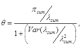
The index of effectiveness (θ) is estimated as seen in figure 4:

Figure 4. Equation. Index of effectiveness.
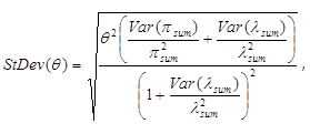
The standard deviation of θ is in figure 5:

Figure 5. Equation. Standard deviation of index of effectiveness.
The percent change in crashes is calculated as 100(1-θ= 0.7 with a standard deviation of 0.12 indicates a 30-percent reduction in crashes with a standard deviation of 12 percent.
A slightly different approach to the methodology was required for the analysis of the treatment sites in Missouri, which is installing rumble strips on two-lane rural roads whenever a resurfacing project is undertaken. As a result, it would be very difficult to identify comparable roadways with no rumble strips for this road type presently or in the near future. For this reason, a separate reference group of sites without rumble strips was not identified.
An alternate approach to the standard EB before-after methodology was applied. In short, this method makes use of the before period data at the treatment sites to develop SPFs to control for regression-to-the-mean and traffic volume changes. Because the installation of rumble strips is a policy for all resurfacing projects, regression-to-the-mean is not as high a concern as it otherwise may be. The SPFs calibrated from before period data are also used to account for time trends in the earlier part of the study period, before most of the sites have had rumble strips installed. However, after a substantial number of sites have been treated, the number of sites is low for developing yearly factors and is not possible after all have been treated. For these later years, the after period data are used to develop SPFs for calculating yearly factors for the after period. The before period yearly factors are extrapolated based on the ratio of the after period factors to a common year.
To illustrate, consider the fictional information in table 6. Using the SPFs calibrated for both the before and after periods, annual multipliers were estimated for each year. In 2006, there was no data for the after period, so a multiplier does not exist for that year for the after period SPF. Similarly, there is no multiplier for 2009-2011 using the before period data. The average of the multipliers for the common years (2007-2008) is computed. The after period multipliers post-2007 are adjusted by dividing the values by the 2007-2008 average. Finally, the missing yearly multipliers for the before period model are adjusted by multiplying the average from 2007-2008 (1.03) by the value of the adjusted after period multiplier for each year. These are the annual multipliers used in the evaluation.
Table 6. Illustration of alternate approach.
Year |
Using After Period Data |
Adjusted After Period Multipliers |
Using Before Period Data |
Adjusted Before Period Multipliers |
|---|---|---|---|---|
2006 |
N/a | 0.98 | ||
2007 |
1.17 | 1.01 | ||
2008 |
0.99 | 1.05 | ||
Average 2007-2008 |
1.08 | 1.03 | ||
2009 |
1.23 |
1.14 |
N/A |
1.17 |
2010 |
0.84 |
0.78 |
N/A |
0.80 |
2011 |
1.96 |
1.81 |
N/A |
1.86 |
N/A = Not applicable.
Blank cell = No adjustment is required.