U.S. Department of Transportation
Federal Highway Administration
1200 New Jersey Avenue, SE
Washington, DC 20590
202-366-4000
Federal Highway Administration Research and Technology
Coordinating, Developing, and Delivering Highway Transportation Innovations
| REPORT |
| This report is an archived publication and may contain dated technical, contact, and link information |
|
| Publication Number: FHWA-HRT-17-016 Date: April 2017 |
Publication Number: FHWA-HRT-17-016 Date: April 2017 |
Four dependent measures of interest were analyzed: brake distance, the probability of a complete stop, glance duration, and scan time allocation. All available observations were used in the analysis of glance duration and scan time allocation, but only crossings without queues were used in brake distance models, and only totally unimpeded crossings were used in complete stop probability models. All modeling was performed using generalized estimating equations (GEEs), where analysis of repeated measures was possible, and generalized linear models (GLMs). The quasilikelihood under the independence model criterion (QIC) and scaled deviance statistics were used to assess GEE and GLM model fit, respectively. Smaller values of both statistics’ QIC indicate better fitting models. Wald statistics for type 3 GEE analysis are reported. A value of 0.05 was used as the cutoff for determining p-value significance. All reported confidence intervals have been adjusted for simultaneous hypothesis testing.
Data provided on the status of the brake pedal was binary, indicating whether or not the brakes were activated. The distance at which the brake variable first took on the value of 1 was identified as the brake distance. Figure 17 shows the distribution of this distance for the 279 crossings that did not involve vehicle queues.

Figure 17. Graph. Brake distance (non-queued crossings only).
Brake distance overall averaged 329.4 ft (with a standard deviation of 115.8 ft) from intersection center. The choice of when to apply the brakes and thus begin to prepare to heed the stop sign is dependent on the presence of a vehicle queue. Logic dictates that if a lead vehicle is present, whether stationary or concurrently approaching the intersection, the driver of the upstream vehicle will be forced to apply the brakes sooner than in the absence of such a vehicle. Median brake distance among queued crossings was 31.5 ft greater than non-queued crossings (332 and 300.5 ft, respectively). In a previous study using an instrumented vehicle, Bao and Boyle found significant differences in brake distance by age: middle-aged drivers braked earlier than younger and older drivers.(13) However, no such difference was observed between older and younger drivers in the present data.
The speed at which drivers were traveling when they first applied the brakes was also identified. Brake distance and brake speed were found to be positively correlated (Pearson correlation coefficient of 0.76). That is, greater brake distances were associated with higher approach speeds. It was hypothesized that drivers who attained a lower minimum speed also applied the brake further upstream of the intersection, but the two measures were very weakly correlated (Pearson correlation coefficient of 0.11).
Brake distance is defined as the distance from the intersection center at which drivers first applied the brakes. Because brake distance was found to be affected by the presence of vehicle queues, 132 such cases were excluded, leaving 279 for analysis. Separate GEEs were estimated for each predictor variable analyzed. These models employed normal response distributions with identity link functions and repeated measures clustered on participants.
Table 6 lists the QIC statistics for these models. The hypothesis that drivers who attain a lower minimum speed also apply the brakes farther upstream of the intersection was tested but failed to improve model fit over the null (296.5 > 286.9).
Table 6. Fit statistics for brake distance models.
| Model | QIC |
|---|---|
| Minimum speed | 296.5 |
| Null | 286.9 |
| Brake speed + rolling stop risk | 285.8 |
| Brake speed + maximum deceleration | 279.1 |
| Brake speed + gender | 276.8 |
| Brake speed + crash history | 276.6 |
| Brake speed + maneuver | 275.0 |
| Brake speed + rolling stop tendency | 272.6 |
| Brake speed + AAM | 265.5 |
| Brake speed + minimum speed | 265.3 |
| Brake speed | 264.2 |
| Brake speed + age group | 256.7 |
However, a model using brake speed—the speed at which the driver was traveling upon initial brake application—produced a better fit (264.2 < 286.9) and predicted the result shown in figure 18.
![]()
Figure 18. Equation. Estimated brake distance (ft) as a function of brake speed (mi/h).
Brake distance was measured in feet and speed in miles per hour. Speed at brake application was normally distributed with a mean of 61.7 and standard deviation of 11.5. Figure 19 shows the results of this calculation for selected speeds. Note that the difference in brake distances at 50 and 70 mi/h (the approximate 25th and 75th percentiles, respectively) is a considerable 152.9 ft.

Figure 19. Graph. Mean brake distance by speed at brake point.
The only additional explanatory variable that further improved the model fit was age group (256.7 < 264.2). Figure 20 shows that older drivers (ages 45–84) consistently applied the brakes farther upstream than younger drivers (ages 16–44) and that this difference became more pronounced at higher speeds. At 40 mi/h, the difference in brake distance was negligible, but, at 70 mi/h, the difference was statistically significant at 104 ft. While driver age cannot be controlled by local transportation departments, such differences could precipitate situations in which a younger driver rear-ends an older driver because the former may not expect what he or she might consider an early or unnecessary decrease in speed and may ignore or fail to detect other visual cues indicative of the downstream driver braking. The difference may also be due to engine braking among younger drivers or older drivers enjoying the comfort of a gradual brake from farther upstream.

Figure 20. Graph. Mean brake distance by speed at brake point and age.
An attempt was also made to estimate the effect of vehicle classification on brake distance. Of the 279 crossings examined, 96 percent were made in cars, with the remaining crossings executed in pickup trucks (2.5 percent), sport utility vehicles (SUVs) (1.1 percent), and minivans (0.4 percent). Unfortunately, reliable brake pedal status readings were missing from all crossings made with pickup trucks, SUVs, and minivans, making the analysis impossible.
Of the 411 events, 15 were missing speed data, resulting in a total of 396 useable cases. Figure 21 shows the minimum speed attained in each of these crossings as a histogram. The term “minimum speed” (the lowest speed observed in each crossing) is preferred over “stop speed” because the latter implies a minimum speed of 0 mi/h. Indeed, despite the legal requirement to achieve 0 mi/h before proceeding through any intersection, this was only observed in 49.7 percent of cases. In contrast, in an on-road experiment with an instrumented vehicle, Bao and Boyle found that drivers came to a complete (0 mi/h) stop 81 percent of the time when approaching divided highways.(18) Such a strict definition may be naively narrow and subject to instrument sensitivity, so less conservative definitions were also used: 65.9 percent of events included minimum speeds ≤ 3 mi/h, and 82.3 percent of events included minimum speeds ≤ 6 mi/h.

Figure 21. Graph. Minimum speed (all crossings).
The proclivity to make a complete stop—regardless of minimum speed thresholds—is highly dependent on traffic conditions. Previous work by Bao and Boyle found a significant correlation between higher traffic volume and higher probabilities of complete stops.(18) This pattern was found in the present dataset as well. Figure 22 shows a boxplot of minimum speed for each of the four possible traffic conditions. The median minimum speed of crossings with no CT or vehicle queues was 4 mi/h. Removal of CT or vehicle queues lowered the median to 2.5 or 0 mi/h, respectively. Those crossings with both CT and vehicle queues exhibited a median minimum speed of 0 mi/h.

Figure 22. Graph. Minimum speed by traffic condition.
Minimum speed is defined as the minimum speed observed in each crossing. Because minimum speed was found to be affected by the presence of CT and vehicle queues, 332 such cases were excluded, leaving 79 for analysis. The three minimum speed thresholds used to define complete stops (0, 3, and 6 mi/h) were applied to the continuous variable minimum speed to create a binary variable for each. Separate GEEs were estimated for each predictor variable analyzed. These models employed binomial response distributions with logit link functions and repeated measures clustered on participants.
Table 7 lists the QIC statistics for these models (using the 0 mi/h threshold). Four separate models outperformed the null, with AAM yielding the best fit.
Table 7. Fit statistics for complete stop probability models.
| Model | QIC |
|---|---|
| Maximum deceleration | 98.5 |
| Age group | 97.1 |
| Crash history | 96.1 |
| Null | 94.0 |
| Gender | 88.6 |
| Rolling stop tendency | 88.1 |
| Rolling stop risk | 72.6 |
| AAM | 50.1 |
Age group failed to produce a better fit than the null model, but AAM surpassed all others, suggesting that the latter better reflects driver experience. Figure 23 shows the probability of making a complete stop (denoted as Pr(Complete Stop)) by AAM for each definition of “complete.” Drivers who reported an annual average of 20,000 to 30,000 mi were 9.1 times more likely to make complete stops (0 mi/h) than those driving 10,000 to 20,000 mi (p < 0.001). This difference is statistically insignificant at the 3-mi/h threshold; however, too little variation existed under the 6-mi/h threshold, and too few drivers fell into the extreme mileage categories to analyze further.

Figure 23. Graph. Probability of making a complete stop by AAM for each definition of “complete.”
Participants were asked, “If you were to not make a full stop at a stop sign, how do you think it would affect your risk of crash?” Figure 24 shows that drivers who expressed a high risk associated with performing rolling stops were more likely to perform them. (Note that this graph shows the probability of a rolling stop, which is the complement to the probability of a complete stop.) Those indicating high risk were 6.8 to 14.0 (p = 0.002 to 0.015) times more likely to perform rolling stops (3 and 6 mi/h thresholds, respectively) than those who indicated that doing so only posed a medium risk, although this difference was not statistically significant under the 0-mi/h threshold.

Figure 24. Graph. Probability of making a rolling stop by expressed risk associated with performing a rolling stop for each definition of “complete.”
Participants were also asked, “In the past 12 mo while driving, how often did you not make a full stop at a stop sign?” Figure 25 shows that those who claimed to “never” or “rarely” commit rolling stops were no less likely to do so than those who admitted to doing it “often” or “sometimes” (p > 0.05 for all stop definition thresholds). These two findings indicate a social demand characteristic; participants may have felt inclined to tell transportation researchers that rolling stops are highly risky and that they do the right thing and never or rarely commit them. Regardless, these results strongly suggest that self-assessments concerning such behaviors are unreliable.

Figure 25. Graph. Probability of making a rolling stop by expressed tendency to perform a rolling stop for each definition of “complete.”
As drivers neared the intersections, they glanced around their surroundings. Figure 26 shows each eyeglance to the eight identified visual ROIs (excluding unavailable and transition). The forward ROI dominates drivers’ vision for the majority of the approach, with glances to the left and right becoming more common in the last 197 ft. Overall, glances to the forward ROI accounted for 56.3 percent of total glance time. Excluding the last 197 ft, forward glances account for 83 percent of total glance time, well in line with Brakstone’s and Waterson’s finding that drivers generally spend 80 percent of their time looking in the forward ROI.(19)

Figure 26. Graph. Discrete eyeglances along intersection approach.
Many prior studies have examined the relationship between single-glance duration away from the road and various safety metrics, generally concluding that two seconds spent glancing away from the roadway significantly increases crash risk. (See references 20–23.) Because this study aimed to describe glance patterns at different points along the approach, a discrete framework had to be implemented. To compare the time that drivers spent glancing at each ROI along the approach, approaches were divided into five 98.4-ft segments, where segment 1 indicated 0–98 ft, 2 indicated 98–197 ft, etc. Because of the speed variation inherent to approaching a stop-controlled intersection (as well as CT and queue presence), this segmentation results in drivers occupying segment 1 the longest. Table 8 shows speed and time statistics for each segment.
Table 8. Mean speed and time spent in each segment.
| Segment | Speed (mi/h) | Time (s) | ||
|---|---|---|---|---|
| Mean | Standard Deviation |
Mean | Standard Deviation |
|
| 1 | 12.6 | 9.7 | 10.8 | 8.9 |
| 2 | 38.2 | 10.5 | 2.7 | 1.5 |
| 3 | 51.3 | 10.6 | 2.1 | 2.0 |
| 4 | 59.2 | 9.2 | 1.7 | 0.4 |
| 5 | 63.5 | 9.2 | 1.6 | 0.3 |
VTTI examined video feeds for each crossing and denoted glance targets for each 0.07-s video frame. Each crossing consisted of an approach at least 492.1 ft in length, which was then divided into 98.4-ft segments. (Observations more than 492.1 ft from the intersection were discarded.) Absolute total glance duration for each ROI segment combination was used as the dependent variable. These data were then merged with the time-series data using VTTI’s timestamp, which resulted in a dataset with timestamped geospatial coordinates and eyeglance targets (among other variables). Separate GEEs were estimated for each ROI and each predictor variable analyzed. These models employed Poisson response distributions with log link functions and repeated measures clustered on crossings.
Table 9 shows the resulting fit statistics (QIC) for each ROI and model specification. The high incidence of missing values is the result of too few glances to certain ROIs. For example, mean total glance duration to cell was less than 0.05 s for each segment, while mean total glance duration to forward was greater than 1.3 s. This scarcity made models with factors in addition to segment impossible to estimate for several ROIs. Table 9 also shows that the null models outperform several others (produce lower QIC statistics) on several ROIs. The goal of this research, however, was to create a model of glance behavior along the driver’s approach to a stop-controlled intersection.
Table 9. Fit statistics (QIC) for glance duration models.
| Model | Far Left |
Near Left | Forward | Rearview | Near Right | Far Right | Other | Cell |
|---|---|---|---|---|---|---|---|---|
| Null | 813.5 | 823.2 | 616.5 | 216.5 | 1,122.2 | 700.1 | 795.0 | 43.3 |
| Segment | 647.5 | 1,142.4 | 633.4 | 385.1 | 1,542.4 | 786.5 | 898.6 | 74.8 |
| Segment + maneuver | 660.7 | — | 671.6 | — | 1,551.5 | — | 921.2 | — |
| Segment + traffic conditions | — | — | 627.1 | — | — | — | 962.0 | — |
| Segment + gender | 686.9 | 1,154.4 | 627.5 | — | 1,515.6 | 734.3 | 985.6 | — |
| Segment + age group | 657.3 | — | 610.6 | 423.2 | 1,556.9 | — | 856.8 | — |
| Segment + AAM | — | — | 650.3 | — | — | — | — | — |
| Segment + crash history | 659.4 | 1,142.0 | 634.4 | — | 1,583.6 | — | 906.2 | — |
| Segment + rolling stop risk | 594.0 | 1,069.5 | 1087.2 | — | 1,466.7 | — | 826.0 | — |
| Segment + rolling stop tendency | 698.8 | 1,161.6 | 657.1 | — | 1,477.8 | 741.4 | 937.9 | — |
| Segment + maximum deceleration | 724.7 | 1,195.9 | 654.8 | — | 1,586.6 | — | 948.3 | — |
| Segment + full stop (0 mi/h) | 627.1 | 1,229.6 | 632.0 | — | 1,592.9 | 794.8 | 980.7 | — |
| Segment + full stop (3 mi/h) | 662.3 | 1,183.3 | 638.5 | — | 1,579.8 | 769.1 | 956.6 | — |
| Segment + full stop (6 mi/h) | 652.4 | — | 628.9 | — | 1,568.2 | 737.7 | 917.0 | — |
| —Models were too sparse to estimate (i.e., ROIs that were rarely glanced at and may not coincide with all levels of another model variable). | ||||||||
Table 10 compiles the Wald statistics for type 3 GEE analysis from each ROI’s segment-only model, where each row represents one ROI-specific model and the statistics associated with the segment variable. For all ROIs except cell, segment is a highly statistically significant predictor of total glance duration.
Table 10. Wald statistics for segment variable from each ROI’s segment model.
| ROI | Degrees of Freedom |
Chi-Squared | p-Value |
|---|---|---|---|
| Far left | 4 | 884.96 | < 0.0001 |
| Near left | 4 | 164.45 | < 0.0001 |
| Forward | 4 | 544.85 | < 0.0001 |
| Rearview | 4 | 63.31 | < 0.0001 |
| Near right | 4 | 215.20 | < 0.0001 |
| Far right | 4 | 565.45 | < 0.0001 |
| Other | 4 | 20.82 | 0.0004 |
| Cell | 4 | 3.53 | 0.4559 |
Figure 27 shows the mean total glance duration estimated for each ROI segment combination. Approaches were divided into five 98-ft segments with segment 1 indicating 0–98 ft from intersection center, segment 2 indicating 98–197 ft, etc. Between 492 and 98 ft from the intersection (segments 5 through 2), the average driver spent very little time glancing directly at the far left (0.24 s total), near left (0.19 s), rearview (0.03 s), near right (0.30 s), and far right (0.08 s). Within 98 ft of the intersection (segment 1), drivers devoted much more time to each (far left was 2.40 s, near left was 0.39 s, rearview was 0.08 s, near right was 0.48 s, and far right was 1.82 s). Among these ROIs, the majority of glance duration (at least 61.5 percent) occurred within 98 ft of the intersection.

Figure 27. Heat map. Mean total glance duration among all crossings.
A very similar pattern emerged in the absence of CT and vehicle queues, as shown in figure 28. Durations to most ROIs were shorter in the absence of traffic, suggesting that some glance time was attributable to waiting.

Figure 28. Heat map. Mean total glance durations among crossings with no CT or vehicle queues.
In an effort to analyze glance times along the approach in the context of other explanatory variables, ROIs were collapsed to three classes: forward (unchanged), scanning (the sum of far left, near left, near right, and far right) and other (the sum of rearview, other, and cell). Again, the null models outperformed others on the collapsed ROIs using QIC as the metric for goodness of fit.
Figure 29 presents the mean total glance duration estimated by the segment-only models for the collapsed ROIs. The Wald chi-squared value for segment in each model was highly statistically significant (p < 0.001). Drivers spent more time glancing in the forward direction as they approached the intersections (though this could be the result of merely occupying each segment longer as speed decreases), with time in segment 1 significantly greater than all others (p < 0.001). Similarly, drivers spent practically no time scanning until 98 ft from the intersection; mean total scanning duration among these segments ranged from 0.1 to 0.3 s and were not statistically different from one another. Total scanning duration in segment 1, however, averaged 5.1 s, a statistically significant (p < 0.001) 4.8-s increase over segment 2. As a percentage of the approach, drivers spent 86.5 percent of their time scanning in these last 98 ft. Glance durations to the other ROI remained low and fairly stable, ranging from 0.05 s (segment 4) to 0.23 s (segment 1).

Figure 29. Graph. Estimated mean total glance duration for collapsed ROIs across segments.
A very similar pattern emerged in the absence of CT and vehicle queues, as shown in figure 30. As with the disaggregated data, glance durations to most ROIs were shorter in the absence of traffic, suggesting that some glance time was attributable to waiting.

Figure 30. Graph. Estimated mean total glance duration for collapsed ROIs across segments among crossings with no CT or vehicle queues.
“Scan time allocation” refers to how drivers allocated their intersection scanning time relative to stopping. Over the course of this research, two subpopulations were identified: (1) drivers who came to a complete stop and then scanned the intersection before proceeding and (2) drivers who scanned ahead of time, performed a rolling stop, and then proceeded through the intersection.
To formally test the differences among these groups, the moment at which each crossing’s minimum speed was attained was used as a before and after delineation. Scan time was calculated as the sum of glance durations to ROIs (far left, near left, near right, and far right) and then expressed as a percentage of total glance time before and after stopping (reaching the crossing’s minimum speed). Because the before and after scan percentages are complementary, the prestop scan time percentage was modeled as a function of stop type (complete or rolling using each definition) and one other predictor variable. Separate GLMs were estimated for each using binomial response distributions and logit link functions.
Table 11 lists the scaled deviance and degrees of freedom for the scan time allocation models (for the 0 mi/h definition of a complete stop only). Though the null model fits reasonably well (P( χ 2395 ≥ 34.1) ≈ 1), adding stop type represents a significant improvement (P( χ 2Δdf ≥ ΔD) = P( χ 21 ≥ 13.0) < 0.001).
Table 11. Fit statistics for scan time allocation models.
| Model | Degrees of Freedom |
Deviance |
|---|---|---|
| Null | 395 | 34.1 |
| Stop type | 394 | 21.1 |
| Stop type + gender | 392 | 21.1 |
| Stop type + age group | 386 | 21.1 |
| Stop type + maximum deceleration | 388 | 21.1 |
| Stop type + crash history | 392 | 21.0 |
| Stop type + maneuver | 390 | 20.8 |
| Stop type + AAM | 386 | 20.8 |
| Stop type + rolling stop tendency | 392 | 20.9 |
| Stop type + rolling stop risk | 389 | 20.4 |
| Stop type + traffic conditions | 388 | 17.8 |
Prestop scan time differed significantly with stop type ( χ 2(1) = 4787.5 and p < 0.001 under the 0 mi/h threshold). Those drivers who came to a complete stop spent just 39.2 percent of their prestop time scanning the intersection, while rolling stoppers spent 74.5 percent. This relationship holds for minimum speeds ≤ 3 mi/h ( χ 2(1) = 3007.37 and p < 0.001) and ≤ 6 mi/h ( χ 2(1) = 1651.07 and p < 0.001). Figure 31 shows these results graphically. This finding confirms the existence of two distinct intersection-scanning protocols: (1) approach intersection, stop, scan, and proceed and (2) scan intersection during approach, slow, and proceed.

Figure 31. Graph. Prestop scanning percentage by stop type for each definition of “complete.”
Further inclusion of prospective predictor variables failed to produce significant improvements (all (P( χ 2Δdf ≥ ΔD) > 0.005), but given the nature of the data, examining this trend under various traffic conditions is worthwhile. A GLM with stop type (based on the 0-mi/h definition), traffic conditions, and the interaction thereof found all terms to be significant predictors of prestop scan time (stop type χ 2(1) = 1,462.95 and p < 0.001; traffic conditions χ 2(3) = 1,014.35 and p < 0.001 and interaction χ 2(3) = 151.73 and p <0.001). This significance was robust to all definitions of a complete stop. Figure 32 shows that the largest difference occurred when both CT and vehicle queues were present, with complete stoppers using just 25.1 percent of prestop time for scanning versus 66.0 percent among rolling stoppers. However, even in the absence of any visible traffic, complete stoppers still spent significantly less prestop time scanning (55.0 percent) than rolling stoppers (79.6 percent).
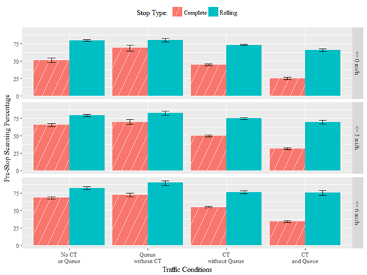
Figure 32. Graph. Prestop scanning percentage by stop type and traffic condition for each definition of “complete.”

