U.S. Department of Transportation
Federal Highway Administration
1200 New Jersey Avenue, SE
Washington, DC 20590
202-366-4000
Federal Highway Administration Research and Technology
Coordinating, Developing, and Delivering Highway Transportation Innovations
 |
| This report is an archived publication and may contain dated technical, contact, and link information |
|
Publication Number: FHWA-HRT-04-147
Date: December 2005 |
||||||||||||||||||||||||||||||||||||||||||||||||||||||||||||||||||||||||||||||||||||||||||||||||||||||||||||||||||||||||||||||||||||||||||||||||||||||||||||||||||||||||||||||||||||||||||||||||||||||||||
Enhanced Night Visibility Series, Volume XVI: Phase III—Characterization of Experimental ObjectsPDF Version (1.07 MB)
PDF files can be viewed with the Acrobat® Reader® CHAPTER 2—METHODSEXPERIMENTAL DESIGNThis study was a 6 by 17 design with two independent variables: VES configuration and type of object. Six types of VESs were tested, of which, three were VIS systems and three were IR-based systems with high head down (HHD) displays. Ten different objects were tested in different positions on the road, generating 17 different object and position combinations. Table 1 presents the VES categories, and table 2 includes the object categories. The VESs and objects are described in more detail in the Independent Variables section.
The dependent variables in the design of this experiment were based on photometric measurements of the objects. The measurements were performed at the mean detection and recognition distances found in the initial experiment. The photometric measurements of object luminance and background luminance were used to calculate values for contrast and visibility level for each VES and object scenario. A detailed explanation of the measurement and calculation of these four variables (the dependent variables for this study) is provided in the Dependent Variables section. Independent VariablesThe independent variables for this experiment, VES configuration and type of object, are described in more detail below. VES TypesFor this experiment, each VIS system was comprised of two headlamps mounted on one of the four experimental vehicles. The IR systems were comprised of two headlamps, a detector system, a viewing screen, and emitters for the active near IR systems. Prototype Far Infrared Vision System: A prototype far infrared (FIR) vision system was tested on a sport utility vehicle (SUV). The system display used a directly reflected virtual image with an 11.7° horizontal by 4° vertical field of view (FOV). The reflective mirror, located in an HHD position on centerline with the driver, was mounted directly on the instrument panel surface above the instrument cluster. The reported magnification at the eye was approximately 1:1. The headlamps used were the production halogen headlamps for this vehicle. Prototype Near Infrared Vision System 1: A prototype near infrared (NIR 1) vision system that used a laser IR emitter was tested on a second SUV. The system used a curved mirror display with an 18° horizontal by approximately 6° vertical FOV. The mirror, located in an HHD position on centerline with the driver, was placed directly on the instrument panel surface above the instrument cluster. The reported minification at the eye was approximately 2:3. The headlamps used were the production halogen headlamps for this vehicle. Prototype Near Infrared Vision System 2: A prototype near infrared (NIR 2) system that used broadband halogen IR emitters was tested on the same type of SUV as the FIR system. The system display used a directly reflected virtual image with an 11.7° horizontal by 4° vertical field of view. The reflective mirror, located in an HHD position on centerline with the driver, was placed directly on the instrument panel surface above the instrument cluster. The reported magnification at the eye was approximately 1:1. The headlamps used were the production halogen headlamps for this vehicle. HID 1: The HID 1 headlamps were tested on a third SUV style. The headlamps were mounted on a light rack system that was placed on the front of the vehicle. The Apparatus and Materials section gives a further description of the mounting process. These headlamps have a narrower lighting footprint than the other HID headlamps tested in this study (figure 1 and figure 2). 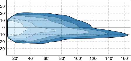 Figure 1. Diagram. Bird’s-eye view of HID 1 beam pattern.
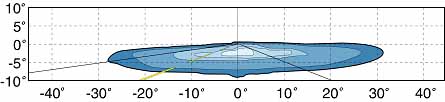 Figure 2. Diagram. Forward beam pattern of HID 1. HID 2: The HID 2 headlamps were tested on a similar SUV as that outfitted with the HID 1 headlamps. The HID 2 headlamps were mounted on a light rack system placed on the front of the vehicle. The HID 2 headlamps have a wider lighting footprint than the HID 1 headlamps. Figure 3 and figure 4 show the HID 2 headlamp beam pattern. 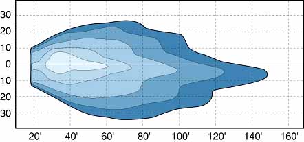 Figure 3. Diagram. Bird’s-eye view of HID 2 beam pattern.
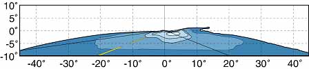 Figure 4. Diagram. Forward beam pattern of HID 2. HLB: The halogen low beam headlamps were tested on the same make of SUV used to test the HID systems. A light rack was used to attach the headlamps to the front of the vehicle. These headlamps were tested to provide a benchmark within this experiment and for comparison to the other VESs tested throughout the various studies in the ENV project. VES Summary: Table 3 shows the different VESs; the vehicles on which the VESs were tested; the headlamps on the vehicle; and, where applicable, the HID system pattern description or the display method, FOV, and image size. Specification of displays, display FOVs, and image sizes were provided by the system engineers responsible for the systems. ENV Volume XVII, Characterization of Experimental Vision Enhancement Systems, provides an indepth look at the technical specifications of each headlamp.
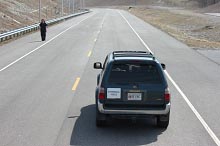
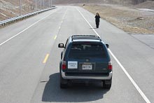
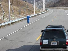
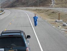
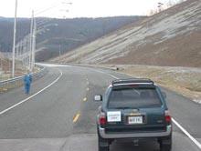
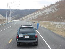
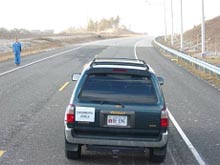
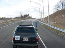
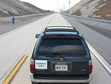
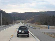
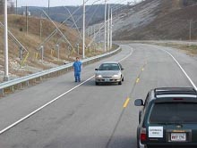
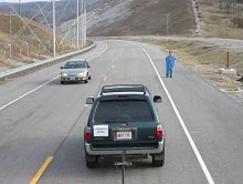
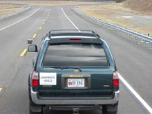
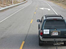
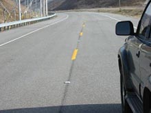
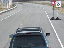
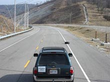
Again, it should be noted that although the display characteristics of the IR systems are provided, they were not tested as part of this object characterization activity. The performance of the headlamps associated with the IR systems and the visual response to them was evaluated. ObjectsThe IR Clear study measured the detection and recognition distances of the 10 different objects for each of the VESs. Some objects appeared on the right side of the road, the left side of the road, or in the center of the road, for a total of 17 different combinations of object and position. The objects selected for this study were grouped into three sets: pedestrians, retroreflective objects, and obstacles. The objects were the same as those used in the IR Clear experiment, and they are described in more detail in ENV Volume XIII. One of the IR Clear study’s tested objects was a bloom scenario, which represented a pedestrian behind an approaching vehicle. The purpose of that test was to evaluate the performance of the IR systems in the presence of glare. For this object characterization activity, the bloom scenario excluded the opposing headlamps and measured only the luminance of the pedestrian. Table 4 and figure 5 through figure 21 describe the objects used for the study as well as their locations. Note that the photographs were taken during daylight hours to demonstrate more clearly the appearance and position of the objects.
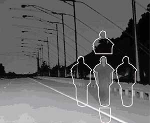
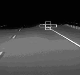
Dependent VariablesThe dependent variables in this experiment are derived from the measured photometric images made by the CCD photometer. The first measurement is the object luminance, or mean luminance of the object in the image. The other measurements are the background luminance, or the mean of the background luminance from above, from below, and to either side of the object. The white outlines in figure 22 and figure 23 show the measurement regions for the pedestrians and tire tread scenarios, respectively.
APPARATUS AND MATERIALSCCD PhotometerAs in the IR Clear study, the object characterization activity used five experimental vehicles, two mid-sized SUVs and three full-sized SUVs. The luminance was measured with a CCD photometer, which allows measurement of the average luminance of a surface. The CCD device was mounted in the driver’s seat of the experimental vehicle. A 50 mm lens provided an image as close to the human visual system as possible. Figure 24 and figure 25 show the photometer and its locations in the experimental vehicle from the left and front side of the vehicle. 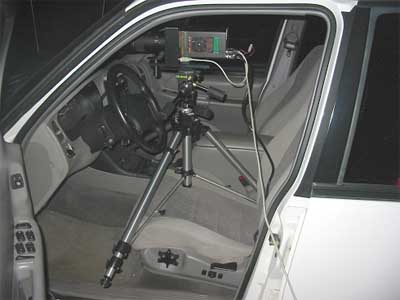 Figure 24. Photo. CCD photometer in experimental vehicle, side view. 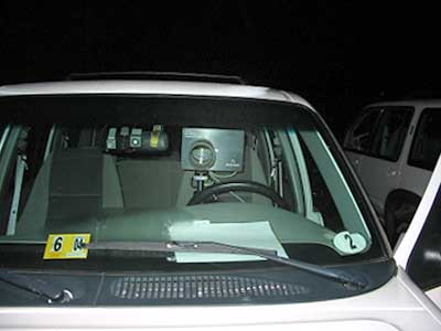 Figure 25. Photo. CCD photometer in experimental vehicle, front view. The output from this system allows for the characterization of the luminance of any point in the image. Headlamp and IR System AlignmentThe HID 1 headlamps, HID 2 headlamps, and HLB headlamps were mounted on a light bar on the front of two mid-sized SUVs during testing (figure 26). To change from one configuration to another, the HLB and HID headlamps were moved onto, off of, and between vehicles. Each light assembly movement required a re-aiming process, which took place before the experimental session started each night. At the beginning of the Phase II studies, a headlamp aimer was not available to the contractor, so an aiming protocol was developed with the help of experts in the field. (See references 1, 2, 3, and 4.) During the photometric characterization of the headlamps, it was discovered that the position of the maximum intensity location of the HLB system was aimed higher and more toward the left than typically specified. This aiming deviation likely influenced the visibility testing results in the IR Clear study; however, this object characterization activity reproduced that aiming deviation to evaluate the objects as they were presented to the experimental participants. ENV Volume XVII, Characterization of Experimental Vision Enhancement Systems, discusses the details of the aiming procedure and maximum intensity location. 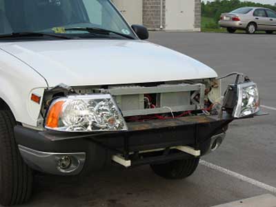 Figure 26. Photo. Headlamp testing rack. Smart RoadThe Virginia Smart Road was used for the IR Clear study and the object characterization activity. Thirty-three locations were used to present objects, with some locations being used for left, right, or center presentation of objects. Some locations were acceptable for certain objects or for certain approach directions to achieve consistent ambient lighting and road geometry. Figure 27 presents a schematic of the Smart Road with examples of object locations. All of the object and location combinations that were used in the IR Clear study were used in this activity. The characterization of any one object was considered to be the mean of all the measurements from all the locations where the object appeared. 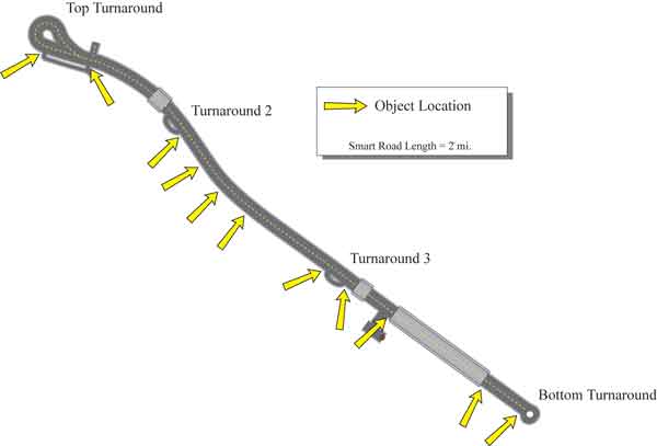 Figure 27. Diagram. Locations of objects in experiment.
MEASUREMENT PROCEDUREThe measurements were conducted in several nighttime sessions at the test facility. In each session, an experimental vehicle with the VES being evaluated was outfitted with the CCD photometer in the driver’s seat. An experimenter, positioned in the driver’s seat, was able to operate the vehicle. A second experimenter, located in the passenger’s seat, was responsible for the operation of the photometer software. For each condition, the driver, with the assistance of an onroad experimenter, placed the vehicle at the mean detection distance from the object being evaluated. A second onroad experimenter then simulated the pedestrian objects or placed the other objects in the appropriate location, and the photometric measurement was taken from the vehicle. After completion of the photometric measurement, the vehicle was moved to the location of the next object, and the process was repeated. This process was used for all VES, object type, and location combinations. Software designed to operate the CCD photometer was used to obtain the luminance data of each object in each presentation location with all VESs. For each VES, a photometric file was created that could then be analyzed for the dependent variables. One image was taken at the previously determined mean detection distance and one at the mean recognition distance for each object. The software created an outline of the object. Using this traced shape, the luminance of the object and the luminance of its surrounding background regions (above, below, left, and right) were obtained. The background luminance measurements of the left or right regions were gathered by placing the traced shape of the object to the left or right of the target object. A similar procedure was used to measure the luminance of top and bottom background regions. The average luminance of the object itself was measured by highlighting around its edge. To determine luminance of different parts of the pedestrians, the software traced a shape that was only one-third of the pedestrian, from the knees down or the chest up. This shape was then used to gather the top and bottom luminance values. The measurements for all objects and all VESs were made with this system. DATA ANALYSISAn analysis of the results allows investigation of the effect of the visible-light VESs on the photometric data. Because the IR systems do not emit visible light, the photometric data were used to determine when detections were made at levels below the threshold of visibility, which would imply that the IR systems were used to detect the objects. Finally, an analysis of the participants’ ages was included to compare the age results to the photometric results. Calculated VariablesUsing the photometric data of object luminance and background luminance, two other metrics were calculated—contrast and visibility level. ContrastThe contrast of an object to its background is calculated based on the difference of the luminance of the object and the luminance of the background. Negative contrast occurs when the object is darker than the background. This relationship is shown in figure 28.  Figure 28. Equation. Contrast calculation. For the pedestrian objects, the contrast was evaluated using the mean of the background measurements and the mean of the object measurements. Visibility LevelThe visibility level was calculated based on the object visibility model of Adrian.(5) In his model, the threshold luminance difference ( The Adrian model is calculated using a basic formula with additions to modify the result for various conditions. The basic calculation is shown in figure 29.  Figure 29. Equation. Basic The functions This Figure 30. Equation. Time factor calculation. In this time factor equation, t represents the observation time, and a, which is defined in Adrian’s paper,(5) is a function of the target size and background luminance. Objects that appear in negative contrast (object darker than background) are more easily seen than those that appear in positive contrast (object lighter than background). A factor (FCP) was developed based on the target size and background luminance. The final factor that must be accounted for is the age of the observer. The basic model is developed for a 23-year-old observer. To account for a different age group, the age factor (AF) equation shown in figure 31 must be used. The values of the constants a, b, and c are presented in Adrian’s document.(5) Figure 31. Equation. Age factor calculation. The final model of the  Figure 32. Equation. Complete As a metric for visibility, VL is the ratio of the actual luminance difference and Figure 33. Equation. Visibility level calculation. In this calculation, when the visibility level is 1 it implies a 50 percent probability of detection, thus the distance at which the VL equals 1 should be the mean detection distance. In a driving task, however, the practical threshold is higher to allow for driver distraction and workload. The Illuminating Engineering Society of North America RP-8 uses a visibility level of 2.6 to 3.8 in practice.(6) The complete
Object and VES ClassificationAs in the data analysis for the IR Clear study, the objects were divided into three groups: pedestrian, retroreflective object, and obstacle. The pedestrian group included all scenarios that involved detecting and recognizing a pedestrian, including the bloom scenario, both black- and denim-clothed pedestrians, pedestrians in turns, and far-off-axis pedestrians. The retroreflective object group included the turn arrow, the RRPMs, and the signs. The obstacle group included the dog and the tire tread; these two objects were both smaller, low-contrast objects that extended into the lane of the participant vehicle. The VESs were also grouped into two categories: VIS systems, including the HLB and HID headlamps, and infrared systems, including the FIR and NIR systems. Photometric Measurement ComparisonsAn assessment of the means of the data for VIS systems with respect to luminance, background luminance, contrast, and visibility levels was conducted to identify potential differences between each system type. It was thought that a statistical comparison was not an appropriate method of analysis at this juncture, and thus a confidence interval of the means for VES and object type was created for each of the photometric measurements. It should be noted that if the objects were measured only once for each VES and object combination, it meant that an object appeared on the road in only one location, and no estimate of the measurement error could be obtained. Identifying the System UsageThe process of detecting objects in the roadway when using an IR system is not direct visual observation of the object. As discussed, the IR systems use a camera sensitive to portions of the electromagnetic spectrum other than the visual region and create a visual representation of the detector response on an in-vehicle display. The photometric data were used as a means to indicate use of the IR systems’ in-vehicle display by the study participants. If the calculated visibility level for an object at the mean detection distance was significantly less for the IR system than the visibility level at detection when using a VIS system, then it was assumed that the IR system was used, and the object was not detected by direct observation through the windshield. Age AnalysisThe final aspect of interest in this analysis is the effect of age. Using the age factor associated with the visibility-level model identified earlier, the age factor results from the IR Clear study were compared to the modeled results. The ratio of the performance by older drivers to that of younger drivers was then compared to an equivalent ratio calculated from the model.
|