

ABC AHP Decision Tool Manual
Final March, 2012
- 1 Introduction
- 2 Decision Model Hierarchy Operations
- 3 AHP Analysis
- 4 Results Window
- 5 Cost Weighted Analysis
- 6 Data Structure
- Appendix I - Analytical Hierarchy Process Overview
Project Number: TPF-5(221)
1 Introduction
1.1 Software Overview
The Oregon State University ABC AHP decision tool was developed using Microsoft Visual Studio .NET as a stand-alone application. This product includes ZedGraph library developed by John Champion, Chris Champoin, and Ronan O Sullivan. This library is published under the GNU Library or Lesser Public License (LGPL). The software has been fully tested on all currently-supported Windows versions (i.e. MS Windows XP, Vista, and Seven). The software incorporates advanced software development concepts including modular and object oriented design. As a result, the software has a high level of flexibility in addressing existing user’s needs and in support of future development. Figure 1 shows a screen shot from the application’s graphical user interface (GUI).
1.2 Graphical User Interface
The software interface has a tabular design that divides the overall analysis process into several independent steps. To initiate an analysis, the user must complete all tasks associated with a tab before proceeding to the next tab. The tabs are usually visited from the left to the right. After processing a project once, the user can go back and forth between tabs.
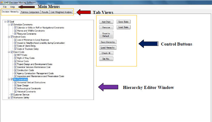
Figure 1. ABC AHP Decision Tool Graphical User Interface
The first tab is associated with constructing a decision hierarchy. In this tab, the user has access to all necessary functions to support loading, saving, and modifying a decision hierarchy. The user has the option to disable a decision category either temporarily or permanently for every hierarchy. The second tab (Figure 3) is associated with conducting pairwise comparisons. The user can save the state of an analysis at anytime and later return to that specific position, without losing any data. After finishing all pairwise comparisons, the user can review the results in the third tab (Figure 5). For each node, existing in the decision model, the tool will generate a set of two plots: a bar chart indicating the utility levels of the two alternatives being compared and a pie chart showing the weights for each of the sub-categories. The last tab provides the user with the option of completing an additional cost-weighted analysis. This tab may be used only after all cost criteria have been eliminated from the decision model constructed using the first (left most) tab.
1.3 Software Requirements
In order to use the ABC AHP Decision Tool, Microsoft .NET Framework 4.0 or later must be installed. If this requirement is not met, the software will produce an error message, indicating that the Microsoft .NET Framework must be installed. Users can download and install this package at: http://www.microsoft.com/net/download.aspx.
1.4 How to Initiate a Session
The AHP ABC Decision Tool folder contains files that are required for proper operation of the software. To initiate a session of the ABC AHP Decision Tool, the user must click on the executable file "AHP Tool" (The shape of the executable file icon is shown in Figure 2). This file and all the other supporting files must be located in the same folder on the hard drive. If any files are missing, the user will not be able to run the software.
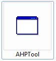
Figure 2. Software Executable File Icon Shape
2 Decision Model Hierarchy Operations
2.1 Add New Child
To add a new sub-criteria or child to a specific node of the hierarchy, the user must select the parent node first from the decision hierarchy view window (first tab). The background color of a selected node changes to blue. Next the user must click on the "Add Child" button. After providing a descriptive name for the new node, the user selects "OK".
2.2 Remove Nodes
To remove a node (with or without children), the user selects the node to be removed. After selecting the node, the user selects the "Remove" button. (Warning: if the node has any children, the child node(s) will also be removed from the hierarchy).
2.3 Reset to Default
The user can reload the default decision hierarchy, developed for ABC decision making by selecting the "Reset to Default" button. If the user wishes to reload a current modified hierarchy later, the user must save the hierarchy before loading the default hierarchy. Once the default hierarchy is loaded, unsaved hierarchies are lost.
2.4 Save Hierarchy
To save a modified hierarchy, the user selects the "Save Hierarchy" button. A "Save the File" window will appear. With this window, the user can specify the name and location of the file on the hard drive (or any other external drives, including USB flash drives or network drives).
2.5 Load Hierarchy
To load an existing hierarchy, the user selects the "Load Hierarchy" button. This will open a new window titled "Open". In this window, the user can select any hierarchy that was saved previously.
2.6 Activate All Nodes
By selecting the "Check All" button, the user can select (check) all nodes at once. This option can save time, especially when working with large hierarchies.
2.7 Temporary Activation/Deactivation of the Nodes
In some cases, the user may wish to analyze the model by temporarily activating or deactivating a node or even a family of nodes. For this purpose, the user does not need to modify the hierarchy (by adding or removing the nodes). Instead, the user can use the small check boxes next to each node. Enabling/disabling these check boxes temporarily enables/disables a node or a family of nodes. If a node is temporarily activated/deactivated, the user will also have to redo the Pairwise Comparison for all affected nodes.
2.8 Define Alternatives
By selecting the "Set Alts." button, the user defines the alternatives that are going to be compared. If not set, the software will use the default alternative names (ABC and Conventional).
2.9 Save Analysis State
The user can save the current state of the software (including the current state of the loaded hierarchy and pairwise comparisons) by clicking on the "Save State" button. The software asks for an appropriate name for the session. The user must use unique names for each new session. Saving a running session with a name previously used for another session, will overwrite previous sessions.
2.10 Load Analysis State
The user can load a previously saved session by clicking on the "Load State" button. After clicking on this button, a browser window will appear which allows the user to look for the saved session on the hard drive or other external drives.
3 AHP Analysis
In the pairwise comparisons window (second tab), the user conducts the comparisons needed to complete an AHP analysis. The results of the analysis are based on individually comparing pairs of decision criteria. The comparison is completed using an established and validated AHP scale (See Table 1).
| Intensity | Definition | Explanation |
|---|---|---|
| 1 | Equal importance | Two activities contribute equally to the objective |
| 3 | Weak importance of one over another | Experience and judgment slightly favor one activity over another |
| 5 | Essential or strong importance | Experience and judgment strongly favor one activity over another |
| 7 | Demonstrated importance | An activity is strongly favored, and its dominance demonstrated in practice |
| 9 | Absolute importance | The evidence favoring one activity over another is of the highest possible order of affirmation |
| 2, 4, 6, 8 | Intermediate values between the two adjacent judgments | When compromise is needed |
3.1 AHP Fundamental Scale
Pairwise comparisons are used to determine the relative importance of each criterion and the degree to which each alternative satisfies the goal when a set of criteria is considered. The decision maker evaluates the relative importance of each criterion in comparison to all other criteria and assesses how well each alternative satisfies each criterion.
Each choice is a linguistic phrase. Some examples of linguistic phrases that can be used are: "A is more important than B", or "A is of the same importance as B", or "A is a little more important than B", and so on.
For example, when system A is compared to system B and a decision-maker has determined that system A is between the classifications of "essentially more important" and "demonstrated more important" than system B (see Table1), then the pairwise comparison would assume the value of 6.
3.2 Pairwise Comparison Operation
In the pairwise comparison window, the user still has visibility to the decision hierarchy (in read-only mode) on the right hand side of the window. By clicking on each node in the hierarchy listing on the right, all pairwise comparisons associated with that node will be displayed (see Figure 3). After completing each set of comparisons, the user can either use the "Next Node" button to move to the next node or click on another node in the hierarchy. The text of completed nodes will change to red when all comparisons associated with that node have been completed.
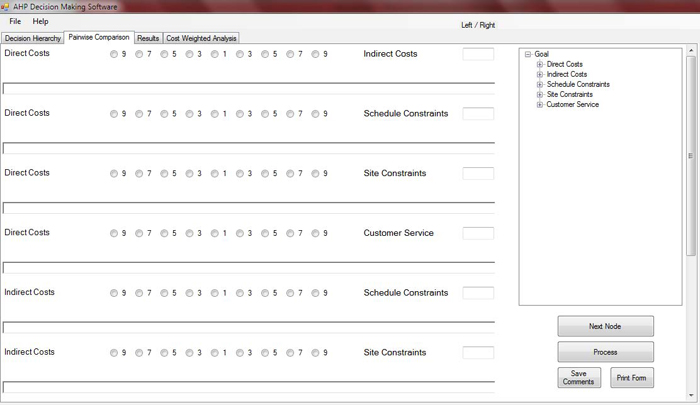
Figure 3. ABC AHP Decision Tool Pairwise Comparison Form
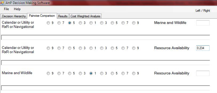
The user can compare criteria in two ways. For qualitative criteria, the user can use the scales provided on the form to rate the relative importance of criteria. If the criteria are quantitative (and accurate values or estimations are available) or the user wishes to use even scale numbers, text entry boxes are provided next to each comparison. The value entered in this box will represent the relative importance of the criterion on the left, over the criterion on the right. For example, if the user enters 4 in the entry box, it means that the weight of the criterion on the left is 4 times the weight of the criterion on the right, whereas by entering 0.25 (the reciprocal of 4, which is ¼), the user shows the opposite case, in which the weight of the criterion on the right is 4 times the weight of the criterion on the left.
If the user uses both the radio buttons and manually enters a rating or a ratio in the text box, the value entered in the text box has the priority and will override the value entered using the scale. The software prevents the user from entering characters into the text boxes. The software also prevents the user from saving the comparison form, before finishing all comparisons.
When the user completes all comparison forms (all nodes in the hierarchy changed to red), the user must then click on the "Process" button. The results will then be available in the results window (third tab).
3.3 Comments on Pairwise Comparisons
A key point to being able to understand and articulate the results of the pairwise comparisons after the analysis is done is tied to the ability to capture the comments provided by various discipline experts and decision makers during the input process. These comments can be used later to explain to the stakeholders the reason why certain pairwise comparisons were rated in a certain way.
To incorporate this feature, a comment field (text box) is placed below each pairwise comparison that can fit up to 170 characters. After putting the comments related to each high level criterion or sub-criterion, the user must press the "Save Comments" button and then move to the next node (failing to press the "Save Comments" button causes the comments to disappear when the user moves to another node.) The saved comments will be visible to the user every time they open a saved session.
3.4 Printing the Pairwise Comparisons Forms
The user can print a summary report of all the input in a certain page of pairwise comparisons by pressing the "Print Form" button in the Pairwise Comparison tab. The generated report contains the data related to the level of preference of one criterion/alternative over another criterion/alternative along with the comments for each pairwise comparison. Figure 5 shows an example of this summary report.
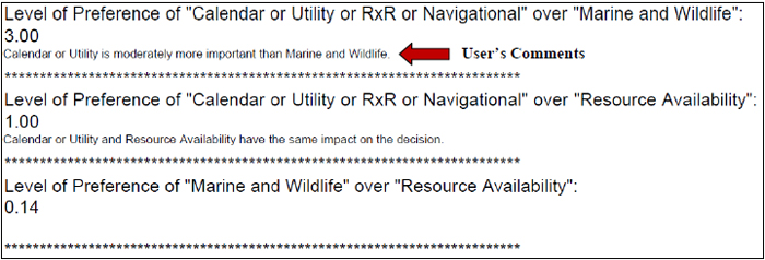
Figure 5. Pairwise Comparison Report Form
4 Results Window
From the results tab, the user can review the results of the AHP analysis completed using the pairwise comparisons or ratios entered by the user (Figure 6). At the center of the page, the utilities for each alternative are presented. The alternative with higher utility is the best alternative based on the completed comparisons.
In this page, for each decision hierarchy node, two sets of plots are generated, a stacked bar chart and a pie chart. These plots are dynamically generated for each hierarchy node. In other words, every time the user selects a node or category from the decision hierarchy on the right, the associated plots are drawn automatically. The bar chart represents the preference or utility level, calculated for the alternatives, by only considering the criteria within that specific node. In other words, when the user selects the "Schedule Constraints" node from the hierarchy, the stacked plot will show the utility level by only considering the weights and preferences associated with calendar and schedule constraints. By default, the software will display the plots for the overall results (plots associated with the "Goal" node) when the user moves on to the results tab. At the "Goal" node level, every generated bar is aggregated based on the utility values calculated using every subcategory.
The pie chart shows the synthesized weight for every sub-criterion in a selected category. If the user selects a third-level criterion, the pie chart will show the user-entered preference for different alternatives. The criterion with the highest weight in pie chart has the greatest contribution towards the total utility displayed in the stacked bar chart.
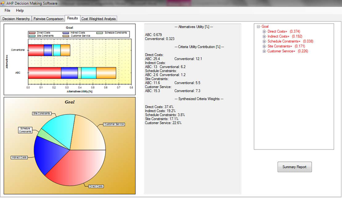
Figure 6. Analysis Result
4.1 Chart Features
There are a number of useful features in the chart module that user can use to manipulate and export the results. These features are managed separately for the stacked bar chart and pie chart and are accessible by right clicking on the window containing the chart.
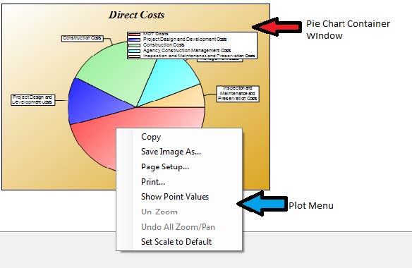
Figure 7. Chart Menu Example
The user can copy the entire chart (including the legend) to the clipboard, using the "Copy" feature. Using the "Save Image As" feature, it is also possible to save the chart on the hard drive (or flash drives and network drives). The user can specify a name and format (*.emf, *.png, *.gif, *.jpg, *.tif, and *.bmp) for the image. The "Print" feature can also be used to send the plot directly to a printer. "Show Point Values" enables the user to determine the size of the portions on a chart. If this feature is enabled, the user can see the stack or slice percentages on the stacked bar chart or pie chart, by hovering the mouse pointer over a specific stack or slice. In the bar chart, the user can zoom in by holding the mouse button while selecting the area of interest. The "Un-Zoom" option allows the user to zoom out of a chart.
4.2 Summary Report
By clicking on the "Summary Report" button below the hierarchy list on the right hand side of the results tab, the user can generate a word file containing all summary results. The word file includes all the bar charts and pie charts associated with the three levels of the hierarchy and a summary of the alternatives utility, criteria utility contribution, and criteria weights.
5 Cost Weighted Analysis
Although costs would typically be included in the hierarchy structure, in some cases, costs might be considered after the benefits of various alternatives have been evaluated.
*Warning: Using the cost weighted analysis feature, when the cost criteria are also included in the hierarchy, will create biased results. The cost weighted analysis tab must be used only after all cost criteria have been eliminated from the decision model constructed using the first (left most) tab.
After completing the AHP process, the user can proceed to the cost weighted analysis tab (fourth tab). In this window, a summary of the AHP analysis, containing the calculated utility for each alternative, is provided. Beneath the summary section, two text boxes are provided. The user must enter the actual or estimated costs for each alternative in the corresponding text box. After entering the costs, the user must select the "Calculate" button. The output for cost weighted analysis will be generated at the bottom of this window, and the preferred alternative will be indicated. Cost weights are calculated using Equation 1. An example analysis is shown in Figure 8. The result can be interpreted as: the calculated utility for the ABC alternative is considerably higher than the conventional alternative. However, since the cost for conducting the project using ABC is very high, the cost weighted analysis results suggest that when the cost criteria are extremely important, the conventional alternative would be the preferred alternative.
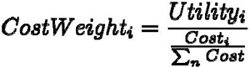
(1)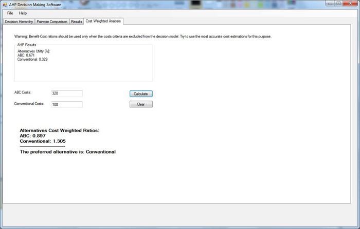
Figure 8. Benefit-Cost Analysis
6 Data Structure
This section describes the mechanism that the software uses to save and restore data. Understanding the material provided in this section is not necessary for basic operation of the software. However, this section will provide the user with a more in-depth understanding of how the software works and enable the user to perform more significant modifications to the hierarchy.
6.1 Hierarchy Data File
The software uses a plain text format (.txt file) to store hierarchy data. Plain text files can be opened or modified using a text editing software, such as Microsoft Notepad. There is no restriction on the location of the hierarchy data file. The file can be stored on any accessible drive. The default hierarchy, developed for ABC bridge projects, is stored in the file "sample.txt", located in the application folder.
*Warning: every time the software loads, the default hierarchy, stored in the file named "sample.txt", in the application folder will be loaded. Removing or renaming this file, may cause software to crash. The user must maintain the default hierarchy in the application folder to prevent malfunction of the software.
In some cases, the user may prefer to modify the hierarchy outside of the software environment and without the hierarchy editor window. In this case, the user can open a hierarchy file with any existing file editor such as Notepad. In the hierarchy file, the criteria categories are separated with a New Line character. Each line starts with the category title. The following elements are the subcategories or child nodes for that category. Elements are separated using a comma and a space. An example of the text string is shown in Figure 9.
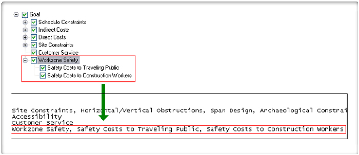
Figure 9. Hierarchy Data Structure
6.2 Software State Data File
The software uses serialization technology to save unfinished and completed analyses. The user can save a session or the state of the software, at any point (including the hierarchy modifications and pairwise comparisons) and restore this state at a later time. The user must provide a name when saving a session. The software will generate six files in the application folder, using a specific naming system. Each file name starts with the session name provided by the user, followed by characters "C", "D", "I", "N", "P", and "R". The file ending with character "I" contains the hierarchy data. The file ending with character "P", contains the pairwise comparison data. The file ending with character "R" contains the system level data. These generated files do not have an extension and cannot be modified outside of the software.
Appendix I - Analytical Hierarchy Process Overview
Analytical Hierarchy Process (AHP) is a decision making technique that is designed to cope with both the rational and the intuitive to select the best alternative from a set of alternatives evaluated with respect to several criteria (Saaty & Vargas, 2001). In this technique, the decision maker performs simple pairwise comparison judgments, which are then used to develop overall priorities for ranking alternatives.
In the simplest form that AHP can be used to construct a decision making problem is a hierarchy consisting of three levels: the overall goal of the decision, the criteria by which the alternatives will be evaluated, and the available alternatives (Figure 10). This hierarchy schema helps the decision maker in the decomposition of complex systems. One organizes the factors affecting the decision (i.e. criteria and sub-criteria) in gradual steps from the general, in the upper levels of the hierarchy, to the particular, in the lower levels. This structure makes it possible to judge the importance of elements in a specific level with respect to some or all the elements in the adjacent level.
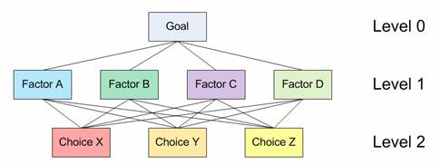
Figure 10. A schematic three-level decision making hierarchy
When hierarchies are constructed, enough relevant detail must be included to present the problem as thoroughly as possible, but not so detailed as to lose sensitivity of change in the elements. When constructing a hierarchy, a number of important issues such as the environment surrounding the problem, attributes contributing to the solution, and participants associated with the problem, must be considered. The elements included in the hierarchy must be homogeneous. The hierarchy does not need to be complete; that is, an element in a given level does not need to function as a criterion for all the elements in the level below. Further, a decision maker can insert or eliminate levels and elements as necessary to clarify the pairwise comparison or to sharpen the focus on one or more parts of the system. Sometimes, less important elements can be dropped from further consideration, if the judgments and prioritization show a relatively small impact on the overall objective.
Procedure of the AHP
The AHP technique can be used to extract ratio scales from both discrete and continuous pairwise comparisons in multilevel hierarchy structures. These comparisons can be performed using actual quantitative measurements or by using a defined scale to represent the relative strength of preferences. AHP takes several factors into consideration simultaneously, allowing for dependence and makes numerical tradeoffs to arrive at a synthesized or conclusion. AHP can be used to establish measures in both physical (tangible) and social (intangible) domains.
The first step in using the AHP to model a problem is to develop a hierarchy or a network representation of that problem. In the next step, a series of pairwise comparisons must be carried out to establish relations within the structure. These comparisons lead to a set of reciprocal matrices (Figure 11). More information about the characteristics of these matrices can be found in Saaty (1990) and Saaty, (1993). Pairwise comparisons in the AHP are performed over pairs of homogenous elements. The fundamental scale of values to establish the intensities of judgments is shown in Table 2. This linear scale uses a one-to-one mapping between the set of discrete linguistic choices available to the decision maker and a discrete set of numbers which represent the importance or weight of the previous choices (Triantaphyllou, 2000). This scale has been validated for effectiveness, in many applications theoretically (Saaty, 2001).
| Loss of Revenue to Local Business | Impact to Neighborhood Livability during Construction | Costs of Users Delay |
Costs of Truckers Delay | |
|---|---|---|---|---|
| Loss of Revenue to Local Business | 1.00 | 0.14 | 0.20 | 0.25 |
| Impact to Neighborhood Livability during Construction | 7.00 | 1.00 | 3.00 | 3.00 |
| Costs of Users Delay |
5.00 | 0.33 | 1.00 | 3.00 |
| Costs of Truckers Delay | 4.00 | 0.33 | 0.33 | 1.00 |
Table 2. The Fundamental Scale used for AHP pairwise comparison
| The Fundamental Scale for Pairwise Comparisons | ||
|---|---|---|
| Intensity of Importance | Definition | Explanation |
| 1 | Equal Immportance | Two elements contribute qually to the objective |
| 1 | Moderate importance | Experience and judgement slightly favor one element over another |
| 5 | Strong importance | Experience and judgement strongly favor one element over another |
| 7 | Very strong importance | One element is favored very strongly over another; its dominance is demostrated in practice |
| 9 | Extreme importance | The evidence favoring one element iver another is of the highest possible order of affirmation |
| Inensive of 2, 4,6, and 8 can be used to express intermediate values. Intensities 1.1, 1.2, 1.3, etc. can be used for elements that are very close in importance | ||
Weber, as reported in Saaty (1980), developed a theory regarding a stimulus of measurable magnitude. According to this psychological theory, a change in sensation is noticed if the stimulus is increased by a constant percentage of the stimulus itself. That is, people are not able to make choices from an infinite set. For example, people cannot distinguish between two very close values of importance, say 3.00 and 3.02 (Miller, 1956). Based on this theory, Saaty established 9 as the upper limit of his scale and, 1 as the lower limit using a unit difference between successive scale values (Saaty, 2001).
Synthesis is obtained by a process of weighting and adding down a hierarchy leading to a multilinear form. A principal eigenvector is normalized to yield a unique estimate of a ratio scale underlying the judgments. This vector represents the relative weights among the elements that are compared.
AHP Example
In this section, a simple AHP problem example is presented. For this example, the user wishes to perform a selection between two different cars: a Honda Accord and a Chevrolet Malibu. For this example, Style, Reliability, and Fuel Economy were chosen as the decision criteria. Comparison matrices and calculation steps to obtain the best alternative using the AHP methodology are summarized.
Pairwise Comparison Table for High Level Criteria
The pairwise comparison tables represent the preference of the decision maker for each criterion and for each alternative. See Table 3. In this example, the user believes that reliability is slightly more important than style and strongly more important than fuel economy. Style is moderately more important than fuel economy.
| Style | Reliability | Fuel Economy | |
|---|---|---|---|
| Style | 1 | 0.5 | 3 |
| Reliability | 2 | 1 | 4 |
| Fuel Economy | 0.33 | 0.25 | 1 |
Normalized Comparison Table
To obtain the normalized table, the summation of each column in Table 3 is calculated. Next, all elements of the comparison table are normalized based on the column’s summation. For example, the summation of the first column of Table 3 is equal to 3.33. To normalize the first column, all elements must be divided by 3.33. The normalization generates 0.3, 0.6, and 0.1. Similar procedure must be followed for columns two and three. The result is shown in Table 4.
| Style | Reliability | Fuel Economy | |
|---|---|---|---|
| Style | 0.3 | 0.285 | 0.375 |
| Reliability | 0.6 | 0.571 | 0.5 |
| Fuel Economy | 0.1 | 0.142 | 0.125 |
Obtained Priority Vector
The priority table is obtained by averaging each row of the normalized table. For example, the priority value for style criterion is obtained by (0.3 + 0.285 + 0.375) / 3 that is 0.320. For reliability, (0.6 + 0.571 + 0.5) / 3 = 0.558. Finally for fuel economy, (0.1 + 0.142 + 0.125) / 3 = 0.122.
| Style | 0.320 |
|---|---|
| Reliability | 0.558 |
| Fuel Economy | 0.122 |
Low-level Pairwise Comparisons
In the next step, the decision maker’s preference over the decision alternatives is generated using the same approach used in Table 3. For example, considering the style criterion only, the user believes that Malibu is slightly more preferred over Accord. Considering the reliability only, Accord is strongly more preferred over Malibu. Considering the fuel economy, Accord is moderately more preferred over Malibu. Same process must be followed to obtain the priority vectors.
| Style | Accord | Malibu | Priority Vector |
|---|---|---|---|
| Accord | 1 | 0.5 | 0.33 |
| Malibu | 2 | 1 | 0.66 |
| Reliability | Accord | Malibu | Priority Vector |
|---|---|---|---|
| Accord | 1 | 5 | 0.83 |
| Malibu | 0.2 | 1 | 0.16 |
| Fuel Economy | Accord | Malibu | Priority Vector |
|---|---|---|---|
| Accord | 1 | 3 | 0.75 |
| Malibu | 0.33 | 1 | 0.25 |
Synthesized Utility Levels
To complete the AHP process, all priority vectors obtained in Table 6 must be combined to one matrix and multiplied to the priority vector obtained for the high level criteria (Table 5).
| 0.32 | ||||
| 0.33 | 0.83 | 0.75 | * | 0.558 |
| 0.66 | 0.16 | 0.25 | 0.122 | |
=
| Accord | 0.665 |
|---|---|
| Malibu | 0.335 |
Therefore, Honda Accord is more preferred over Chevrolet Malibu.