

- Potential Highway Capital Investment Impacts
- Highway Economic Requirements System
- National Bridge Investment Analysis System
- Types of Capital Spending Projected by HERS and NBIAS
- Alternative Levels of Future Capital Investment Analyzed
- Impacts of Systemwide Investments Modeled by HERS
- Impacts of NHS Investments Modeled by HERS
- Impacts of Interstate System Investments Modeled by HERS
- Impacts of Systemwide Investments Modeled by NBIAS
- Impacts of NHS Investments Modeled by NBIAS
- Impacts of Interstate Investments Modeled by NBIAS
- Potential Transit Capital Investment Impacts
- Comparison
Potential Highway Capital Investment Impacts
This section projects the impacts that alternative levels of future investment in highways and bridges might be expected to have on various measures of system conditions and performance. The analyses presented here focus mainly on types of capital investment that can be directly modeled using the Highway Economic Requirements System (HERS) and the National Bridge Investment Analysis System (NBIAS). The capital investment scenarios presented in Chapter 8 draw upon these analyses, but also consider other types of capital investment that are not currently modeled in HERS or NBIAS.
This section also explores the implications of alternative funding mechanisms on the level of combined public and private investment that would potentially be required to achieve certain performance objectives. The options identified include funding from non-user based sources, funding from fixed rate user based sources, and funding from variable rate user based sources such as congestion pricing.
The accuracy of these projections depends on the validity of the technical assumptions underlying the analysis. Chapter 10 explores the impacts of altering some of these assumptions.
A subsequent section within this chapter explores comparable information for different types of potential future transit investments. This is followed by a section providing a crosswalk between the highway, bridge, and transit sections with the information presented in the previous edition of this report.
Highway Economic Requirements System
The investment scenario estimates shown in this report for highway resurfacing and reconstruction and highway and bridge capacity expansion are developed primarily from HERS, a simulation model that employs incremental benefit-cost analysis to evaluate highway improvements. The HERS analysis is based on data from the Highway Performance Monitoring System (HPMS), which provides information on current roadway characteristics, conditions, and performance and anticipated future travel growth for a nationwide sample of more than 119,000 highway sections. While HERS analyzes these sample sections individually, the model is designed to provide results valid at the national level. HERS does not provide definitive improvement recommendations for individual highway segments.
The HERS model analyzes highway investment by first evaluating the current state of the highway system using information on pavements, geometry, traffic volumes, vehicle mix, and other characteristics from the HPMS sample dataset. It then considers potential improvements on sections with one or more deficiencies, including resurfacing, reconstruction, alignment improvements, and widening or adding travel lanes. HERS then selects the improvement with the greatest net benefits, where benefits are defined as reductions in direct highway user costs, agency costs, and societal costs. In cases where none of the potential improvements produces benefits exceeding construction costs, the segment is not improved. Appendix A contains a more detailed description of the project selection and implementation process used by HERS.
Operations Strategies
The HERS model also takes into account the impact that new investments in certain types of intelligent transportation systems (ITSs) and the continued deployment of various operations strategies can have on highway system performance, as well as on the estimated level of capital investment that would be needed to reach given performance benchmarks. This feature was introduced in the 2004 edition of the C&P report. The types of operations investments and strategies considered include freeway management (ramp metering, electronic roadway monitoring, variable message signs, integrated corridor management, and variable speed limits); incident management (incident detection, verification, and response); arterial management (upgraded signal control, electronic monitoring, and variable message signs); and traveler information (511 systems and advanced in-vehicle navigation systems with real-time traveler information).
| How closely does the HERS model simulate the actual project selection processes of State and local highway agencies? | |
|
The HERS model is intended to approximate, rather than replicate, the decision processes used by State and local governments. HERS does not have access to the full array of information that local governments would use in making investment decisions. This means that the model results may include some highway and bridge improvements that simply are not feasible because of factors the model doesn't consider, such as political issues or other practical impediments. Excluding such projects would result in reducing the "true" level of investment that is economically justifiable. Conversely, the highway model assumes that State and local project selection will be economically optimal and doesn't consider external factors such as the distribution of projects among the States or within each State. In actual practice, projects are often not selected on the basis of their benefit-cost ratios; there are other important factors included in the project selection process aside from economic considerations. Thus, the "true" level of investment that would achieve the outcome desired under the scenarios could be higher than the estimates shown in this report.
Currently, approximately 20 States make some use of benefit-cost analysis in managing their transportation programs; only six States use the technique regularly. This means that the majority of transportation decisions in the United States today are being made with limited reference to the projected benefits and costs of a specific course of action relative to another course of action.
|
|
Future operations investments are implemented in HERS through an assumed, exogenously specified scenario; they are not included directly in the benefit-cost calculations made within the model, and HERS does not directly consider any tradeoffs or complementarities between ITS and other types of highway improvements. The baseline scenario used for this report assumes the continuation of existing deployment trends. This scenario was used for all of the HERS-based analyses presented in Chapters 7, 8, and 9. Chapter 10 includes a sensitivity analysis considering the potential impacts of a more aggressive deployment of operations strategies and ITS. Appendix A includes a more complete description of the operations strategies and their impacts on performance.
Travel Demand Elasticity
One of the key economic analysis features of HERS involves its treatment of travel demand. Recognizing that drivers will respond to changes in the relative price of driving and adjust their behavior accordingly, HERS explicitly models the relationship between the amount of highway travel and the price of that travel. This concept, sometimes referred to as travel demand elasticity, is applied to the forecasts of future travel found in the HPMS sample data. The HERS model assumes that the forecasts for each sample highway segment represent a future in which average conditions and performance are maintained, thus holding highway user costs at current levels. Any change in user costs relative to the initial conditions calculated by HERS will thus have the effect of either inducing or suppressing future travel growth on each segment. Consequently, for any highway investment scenario that results in a decline in average user costs, the effective vehicle miles traveled (VMT) growth rate for the overall system will tend to be higher than the baseline rate derived from HPMS. For scenarios in which highway user costs increase, the effective VMT growth rate will tend to be lower than the baseline rate. A discussion of the impact that future investment levels could be expected to have on future travel growth is included in Chapter 9.
Linking Financing Mechanisms and Investment Impacts
The HERS model has recently been modified to allow the exploration of linkages between different types of financing mechanisms used to generate revenues for highway investment and the relationship between alternative investment levels and future system performance. If the revenues needed to support a higher level of future capital investment were generated from non-user sources (such as property taxes or general governmental revenues), then future travel demand would not be significantly affected by the cost of funding infrastructure improvements. However, if such revenues were generated from fixed-rate user charges (such as a VMT charge or fuel tax), the costs experienced by users would rise, resulting in some reduction to the effective VMT growth rate, which would in turn impact the operational performance of the system. To the extent that such revenues were generated directly from individual users by variable-rate user charges (such as congestion pricing, in which users pay according to the costs they impose on the system), the impact on peak period travel would be more dramatic, resulting in significant impacts on system performance for a given level of highway investment. Appendix A includes more details on how this feature was implemented in HERS.
National Bridge Investment Analysis System
The scenario estimates relating to bridge repair and replacement shown in this report are derived primarily from NBIAS. This model incorporates analytical methods from the Pontis bridge management system, which was first developed by the Federal Highway Administration in 1989 and is now owned and licensed by the American Association of State Highway and Transportation Officials. NBIAS, however, incorporates additional economic criteria into its analytical procedures. Pontis relies on detailed structural element-level data on bridges to support its analysis; NBIAS adds a capability to synthesize such data from general bridge condition ratings reported for all bridges in the National Bridge Inventory (NBI). While the analysis in this report is derived solely from NBI data, the current version of NBIAS is capable of processing element-level data directly.
The NBIAS model uses a probabilistic approach to model bridge deterioration for each synthesized bridge element. It relies on a set of transition probabilities to project the likelihood that an element will deteriorate from one condition state to another over a given period of time. The model then determines an optimal set of repair and rehabilitation actions to take for each bridge element, based on the condition of the element. NBIAS can also apply preservation policies at the individual bridge level and directly compare the costs and benefits of performing rehabilitation or repair work relative to completely replacing the bridge.
To estimate functional improvement needs, NBIAS applies a set of improvement standards and costs to each bridge in the NBI. The model then identifies potential improvements—such as widening existing bridge lanes, raising bridges to increase vertical clearances, and strengthening bridges to increase load-carrying capacity—and evaluates their potential benefits and costs. The NBIAS model is discussed in more detail in Appendix B.
Types of Capital Spending Projected by HERS and NBIAS
Chapter 6 identifies three major groups of capital improvement types: System Rehabilitation, System Expansion, and System Enhancement. The types of bridge improvements modeled in NBIAS roughly correspond to the types of bridge improvements classified as System Rehabilitation in Chapter 6. Because NBI data are available for bridges on all functional systems, NBIAS can be used directly to compute the bridge components of future investment scenarios that address the highway system as a whole.
For those functional systems for which data are available, the HERS evaluates types of improvements that roughly correspond to the types of highway resurfacing and reconstruction improvements classified as System Rehabilitation in Chapter 6. HERS also evaluates potential widening improvements, consistent with the types of improvements classified as System Expansion in Chapter 6. As the widening costs considered in HERS reflect both the typical costs of adding lanes per mile of roadway under different circumstances and the costs of modifying a typical number of structures per mile in conjunction with a widening project, the HERS estimates are considered to represent system expansion costs for both highways and bridges. In summary, HERS measures system rehabilitation costs for highways, and system expansion costs for highways and bridges combined; NBIAS measures system rehabilitation costs for bridges.
The HPMS sample segment database used by HERS is limited to Federal-aid highways, and thus excludes roads classified as rural minor collector, rural local, or urban local. Consequently, in order to develop future investment scenarios that address the highway system as a whole, it is necessary to account for these functional systems outside of the modeling process. HERS and NBIAS do not directly evaluate the types of improvements that correspond to the types of improvements classified as System Enhancement in Chapter 6. Thus, developing future investment scenarios that account for these types of improvements also requires external adjustments to be made to the directly modeled improvements generated by HERS and NBIAS. The term "non-modeled spending" is used throughout this chapter and subsequent chapters to refer to spending on capital improvements that is not captured in the HERS or NBIAS analyses.
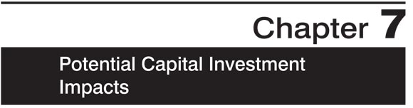
Exhibit 7-1 identifies the portion of total public and private capital investment on highways and bridges in 2006 that corresponds to the types of improvements modeled in HERS and NBIAS. Of the $16.5 billion of capital investment on the Interstate System in 2006, approximately $12.8 billion (77.5 percent) was used for types of improvements modeled in HERS. Approximately $2.5 billion (15.1 percent) was used for types of improvements modeled in NBIAS, while $1.2 billion (7.4 percent) went for types of improvements not addressed by either HERS or NBIAS.
Of the $37.1 billion of capital investment on the National Highway System (NHS) as a whole in 2006, including the Interstate System, approximately $30.0 billion (80.8 percent) was used for types of improvements modeled in HERS. Approximately $4.3 billion (11.6 percent) was used for types of improvements modeled in NBIAS, while $2.8 billion (7.4 percent) went for types of improvements not addressed by either HERS or NBIAS.
| How closely do the capital improvement types presented in Chapter 6 line up with the types of improvements modeled in HERS and NBIAS? | |
|
The reconstruction without added capacity, restoration and rehabilitation, and resurfacing capital improvement types included within System Rehabilitation expenditures in Chapter 6 correspond well to the types of capital improvements modeled in HERS. Reconstruction with added capacity is split between System Rehabilitation and System Expansion in Chapter 6, and must also be split between these categories in the HERS output.
Among the improvement types classified as System Expansion for existing roads, the major widening category from Chapter 6 lines up best with types of improvements modeled in HERS, because such improvements are generally motivated by a desire to address congestion on a facility. The relocation improvement type is also a relatively good fit, although some relocation improvements are motivated primarily by safety concerns more than congestion concerns, and might not be picked up in the HERS analysis.
While HERS does not directly model the construction of new roads and bridges, many such investments are motivated by a desire to alleviate congestion on existing facilities in a corridor, and thus would be captured indirectly by the HERS analysis in the form of additional normal-cost or high-cost lanes. As described in Appendix A, the costs per mile assumed in HERS for high-cost lanes are based on typical costs of tunneling, double-decking, or building parallel routes, depending on the functional class and area population size for the section being analyzed. To the extent that investments in new construction and new bridge categories identified in Chapter 6 are motivated by desires to encourage economic development or accomplish other goals aside from the reduction of congestion on the existing highway network, such investments would not be picked up in the HERS analysis. A study conducted by FHWA's National Systems & Economic Development Team suggests that an estimated $0.5 billion to $2.0 billion per year is spent on highways for economic development purposes. This study is available at: https://www.fhwa.dot.gov/planning/econdev/taskabjan30_1.cfm
The bridge replacement, major bridge rehabilitation, and minor bridge work categories included as part of System Rehabilitation expenditures in Chapter 6 generally correspond to the types of capital improvements for bridges modeled in NBIAS. However, the expenditure data may include work on bridge approaches and ancillary improvements that would not be picked up in the modeling.
The safety, traffic management/engineering, and environmental and other capital improvement categories identified as part of System Enhancement expenditures in Chapter 6 are treated as if they are not captured in the HERS or NBIAS analyses. However, some safety deficiencies may be addressed as part of broader pavement and capacity improvements modeled in HERS. Also, the HERS Operations preprocessor described in Appendix A includes capital investments in operations equipment and technology that would fall under the traffic management/engineering category in Chapter 6.
|
|
On a systemwide basis, the portion of capital spending modeled in HERS is only 61.3 percent, or $48.2 billion out of a total $78.7 billion. This percentage is lower than the comparable values for the Interstate or NHS due to the highway functional systems for which sample section data are not collected through HPMS, which make up $12.1 billion (15.9 percent) of total 2006 capital spending. Approximately $10.1 billion (12.9 percent) of total capital spending was used for types of improvements modeled in NBIAS, while $8.2 billion (10.5 percent) went for system enhancement expenditures which are not addressed by either HERS or NBIAS.
Alternative Levels of Future Capital Investment Analyzed
The specific investment levels reflected in the exhibits in this section were selected from a much larger series of analyses. Each level corresponds to a particular point of interest, such as the amount of investment that is projected to be sufficient to maintain a particular highway or bridge performance indicator at its base year level, or the amount that would finance all potential capital improvements up to a particular benefit-cost ratio cutoff. For each of these analyses, it was assumed that any increase or decrease in combined public and private investment would be phased in gradually, at a constant rate relative to 2006.
| How do the assumptions in this report about the pace of changes in alternative investment levels differ from prior C&P reports? | |
|
For this report, the annual growth rates relative to 2006 levels shown in the exhibits in this section were applied directly in HERS and NBIAS so that the level of investment for each of the years studied rose over time. This approach is considered more realistic than that utilized in the 2006 C&P Report, which assumed that combined public and private capital investment would immediately jump to the average annual level being analyzed, and remain fixed at that level for 20 years.
The 2006 C&P Report was, in turn, an improvement from the 2004 C&P Report with regard to changing investment levels. The 2004 C&P Report assumed that there would be significant front-loading of capital investment in the early years of the analysis as the existing backlog of potential cost-beneficial investments was addressed followed by a sharp decline in later years.
The progression toward a gradual ramping up of spending in the C&P reports reflects an awareness that abrupt increases in spending levels could initially overburden the construction industry and contribute to significant inflation in infrastructure construction costs.
Chapter 9 includes some analysis regarding the timing of investments.
|
|
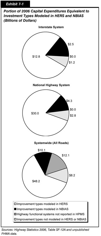
Exhibit 7-2 shows alternative annual rates of increase or decrease in combined future systemwide public and private capital investment and how these would translate into investment levels for individual years, cumulative investment over 20 years, and average annual investment. The average annual investment levels at an annual growth rate of 0.00 percent correspond to the 2006 investment levels identified above, including $48.2 billion for improvement types modeled in HERS, $10.1 billion for improvement types modeled in NBIAS, and $20.3 billion for nonmodeled spending. Maintaining capital investment in constant dollar terms at 2006 levels would translate to a combined investment of $1.574 trillion over 20 years. As all of the values identified are stated in constant 2006 dollars, it is important to note that additional increases would be needed each year to offset the impact of inflation for the period of 2007 to 2026.
| Annual Percent Change Relative to 2006 | Cumulative 2007-2026 Investment (Billions of 2006 Dollars) | Average Annual Investment (Billions of 2006 Dollars) 1 | |||
|---|---|---|---|---|---|
| Total Capital Outlay | Spending Modeled in HERS 2 | Spending Modeled in NBIAS 3 | Non-Modeled Spending 4 | ||
| 7.76% | $3,778 | $188.9 | $115.7 | $24.3 | $48.8 |
| 7.45% | $3,641 | $182.0 | $111.5 | $23.4 | $47.1 |
| 6.70% | $3,331 | $166.5 | $102.0 | $21.4 | $43.1 |
| 6.41% | $3,219 | $160.9 | $98.6 | $20.7 | $41.6 |
| 5.25% | $2,812 | $140.6 | $86.1 | $18.1 | $36.3 |
| 5.15% | $2,779 | $139.0 | $85.1 | $17.9 | $35.9 |
| 5.03% | $2,741 | $137.1 | $84.0 | $17.6 | $35.4 |
| 4.65% | $2,624 | $131.2 | $80.4 | $16.9 | $33.9 |
| 4.55% | $2,594 | $129.7 | $79.5 | $16.7 | $33.5 |
| 4.17% | $2,484 | $124.2 | $76.1 | $16.0 | $32.1 |
| 3.30% | $2,252 | $112.6 | $69.0 | $14.5 | $29.1 |
| 3.21% | $2,229 | $111.5 | $68.3 | $14.4 | $28.8 |
| 3.07% | $2,195 | $109.7 | $67.2 | $14.1 | $28.4 |
| 2.96% | $2,168 | $108.4 | $66.4 | $14.0 | $28.0 |
| 2.93% | $2,161 | $108.0 | $66.2 | $13.9 | $27.9 |
| 1.67% | $1,881 | $94.0 | $57.6 | $12.1 | $24.3 |
| 0.83% | $1,718 | $85.9 | $52.6 | $11.1 | $22.2 |
| 0.34% | $1,631 | $81.5 | $50.0 | $10.5 | $21.1 |
| 0.00% | $1,574 | $78.7 | $48.2 | $10.1 | $20.3 |
| -0.78% | $1,451 | $72.5 | $44.4 | $9.3 | $18.8 |
| -0.86% | $1,439 | $71.9 | $44.1 | $9.3 | $18.6 |
| -1.37% | $1,366 | $68.3 | $41.8 | $8.8 | $17.7 |
| -4.95% | $963 | $48.2 | $29.5 | $6.2 | $12.5 |
| -7.64% | $757 | $37.9 | $23.2 | $4.9 | $9.8 |
The feasibility of achieving the increases or decreases in constant investment presented in Exhibit 7-2 was not evaluated as part of this analysis. In addition, the upper end of the range of investment levels evaluated exceeds the amount of spending that would be cost-beneficial for some system components and for some forms of highway financing mechanisms. While each of the particular rates of change selected has some specific analytical significance, the analyses presented in this chapter are not intended to constitute complete investment scenarios, but instead provide the building blocks for the selected scenarios presented in Chapter 8.
Impacts of Systemwide Investments Modeled by HERS
Exhibit 7-1 shows that of total public and private capital spending of $78.7 billion on all roads in 2006, $48.2 billion was utilized for the types of improvements modeled in HERS. This section projects the potential impacts on system performance of raising or lowering this $48.2 billion in constant dollar terms by various annual rates over 20 years. These percentage increases are also applied to the $78.7 billion in the findings presented in this section; this acknowledges that the improvements reflected in HERS represent only one piece of total capital investment, and that the types of improvements reflected in NBIAS or those that are not reflected in either model should also be considered when projecting the impacts of different overall levels of combined public and private investment.
Alternative Financing Mechanisms
Several of the exhibits in this section compare the potential impacts of alternative financing mechanisms, estimating their relative impact on system performance at a series of alternative funding levels. For funding levels that exceed the current 2006 level of combined public and private highway capital investment, the analyses assume that the additional revenues needed to support such investment would be generated from one of three broad categories: non-user sources, fixed-rate user based sources, or variable-rate user based sources. The selected future highway capital investment scenarios presented in Chapter 8 draw upon some of the analyses presented in this section assuming fixed-rate user based financing or variable-rate user based financing. The non-user sources financing option is not carried forward into Chapter 8.
| How do the types of funding mechanisms considered in the HERS analysis relate to private sector investment? | |
|
The HERS analysis does not distinguish among Federal, State, local, or private sector highway spending. Generally, private sector investment in highways is dependent on revenue streams (primarily tolls) from users of the privately owned facilities. If a private entity were to impose variable rate tolls on a time-of-day basis, HERS would evaluate the potential impacts on peak period VMT to be identical to those that would occur if a public sector entity had imposed congestion charges at the same rates.
In theory, a private sector investment could take on the characteristics of a non-user based financing mechanism. For example, if a government were to pay a private entity to manage a facility on the basis of a "shadow toll" based on usage, but did not impose a fee on highway users to cover these costs, the impact on VMT on that facility would be the same as if the local government had managed the facility itself using general revenues as a funding source.
|
|
The analyses incorporating funding from non-user based sources assume no linkage between increased spending, increased revenue generation, and highway VMT. The analyses incorporating funding from fixed-rate user based sources assume the application of an inflation indexed charge on a per-VMT basis to generate any funding needed to support a higher level of capital investment. The potential size of this charge was initially determined by computing the difference between the investment level being studied and the current 2006 level of combined public and private highway capital investment, and dividing that amount by total projected VMT. This initial value was then recomputed iteratively to account for the impact that the imposition of such a charge would have on the overall cost of driving, which would lead to some reduction in VMT growth. As the same fixed VMT charge would be levied throughout the day, such charges would not affect peak period travel differently than off-peak travel, and as such would be similar in effect to a fuel tax—another form of fixed rate user charge. In cases in which the investment level being analyzed was less than the current 2006 capital spending level, a negative fixed VMT charge was applied, simulating the effects of a reduction in highway user charges. It is important to note that this report does not directly address the issue of the sustainability of current highway financing structures and does not attempt to identify changes in revenue mechanisms or tax rates that might be required to sustain highway capital spending at 2006 levels in constant dollar terms.
| Why do the analyses of funding from fixed rate user sources assume a charge imposed on a per-VMT basis, rather than a per-gallon basis? | |
|
This report does not attempt to differentiate among the relative impacts of alternative fixed rate funding mechanisms such as flat tolls, VMT charges, or the motor-fuel tax; the fixed rate financing analyses are intended to be generic and to provide a contrast with the analyses assuming non-user financing or variable rate user financing (i.e., congestion pricing).
HERS has the capability to model fixed rate user charges on either a per-gallon or per-VMT basis. The per-VMT option was selected for this report, recognizing that such charges may well play an important role in highway financing by 2026. Utilizing the per-VMT option also has the advantage of reducing computational complexity, as it does not need to factor in the effects of changing fleet mileage (and the change in differential between passenger vehicles and commercial trucks) as would have been the case had the per-gallon option been utilized. Another motivation for applying the per-VMT option for the fixed rate user financing analyses is to facilitate comparisons with the congestion pricing analyses that assume a variable rate charge imposed on a per-VMT basis.
The reaction of individual drivers to a per-gallon charge would differ in some ways from their response to a per-VMT charge; in particular, a per-gallon charge would provide a more direct incentive to shift to driving a more fuel-efficient vehicle. However, the cumulative impacts of raising a specific amount of revenue from users on a fixed rate basis via a per-gallon charge versus a per-VMT charge are likely to be less significant, particularly in terms of the types of issues discussed in this report. Some limited HERS analyses conducted assuming fixed rate charges imposed on a per-gallon basis suggest that the total estimated amount of cost-beneficial investment would not differ significantly from analyses assuming per-VMT charges. The level of investment required to achieve other performance benchmarks would vary somewhat, but would not be uniformly biased either upward or downward.
|
|
Exhibit 7-3 identifies the difference between the alternative levels of combined public and private capital investment that were analyzed, and actual capital spending in 2006. If capital investment were to grow by 7.76 percent per year in constant dollar terms over the 2006 level of $78.7 billion, this would result in an average annual investment level of $188.9 billion for the period from 2007 to 2026 in constant dollar terms, a difference of $110.2 billion. In contrast, if highway capital investment were to shrink by 7.64 per year in constant dollar terms, this would free up an average annual amount of $40.8 billion for other purposes.
| Annual Percent Change Relative to 2006 | Average Annual Investment (Billions of 2006 Dollars) Spending Modeled in HERS 1 |
Average Annual Investment (Billions of 2006 Dollars) Total Capital Outlay |
Difference Between Annual Investment Levels and 2006 Total Capital Outlay In Billions of 2006 Dollars2 |
Difference Between Annual Investment Levels and 2006 Total Capital Outlay Per VMT 3 VMT Modeled in HERS |
Difference Between Annual Investment Levels and 2006 Total Capital Outlay Per VMT Total VMT |
Difference Between Annual Investment Levels and 2006 Total Capital Outlay Per Gallon 4 Total Fuel COnsumption |
|---|---|---|---|---|---|---|
| 7.76% | $115.7 | $188.9 | $110.2 | |||
| 7.45% | $111.5 | $182.0 | $103.4 | $0.033 | $0.028 | $0.582 |
| 6.70% | $102.0 | $166.5 | $87.9 | $0.028 | $0.024 | $0.451 |
| 6.41% | $98.6 | $160.9 | $82.3 | $0.026 | $0.022 | $0.406 |
| 5.25% | $86.1 | $140.6 | $61.9 | $0.020 | $0.017 | $0.348 |
| 5.15% | $85.1 | $139.0 | $60.3 | $0.019 | $0.016 | $0.343 |
| 5.03% | $84.0 | $137.1 | $58.4 | $0.019 | $0.016 | $0.338 |
| 4.65% | $80.4 | $131.2 | $52.5 | $0.017 | $0.014 | $0.258 |
| 4.55% | $79.5 | $129.7 | $51.0 | $0.016 | $0.014 | $0.238 |
| 4.17% | $76.1 | $124.2 | $45.5 | $0.015 | $0.012 | $0.262 |
| 3.30% | $69.0 | $112.6 | $33.9 | $0.011 | $0.009 | $0.174 |
| 3.21% | $68.3 | $111.5 | $32.8 | $0.010 | $0.009 | $0.172 |
| 3.07% | $67.2 | $109.7 | $31.1 | $0.010 | $0.008 | $0.168 |
| 2.96% | $66.4 | $108.4 | $29.7 | $0.010 | $0.008 | $0.160 |
| 2.93% | $66.2 | $108.0 | $29.4 | $0.009 | $0.008 | $0.157 |
| 1.67% | $57.6 | $94.0 | $15.4 | $0.005 | $0.004 | $0.079 |
| 0.83% | $52.6 | $85.9 | $7.2 | $0.002 | $0.002 | $0.038 |
| 0.34% | $50.0 | $81.5 | $2.9 | $0.001 | $0.001 | $0.013 |
| 0.00% | $48.2 | $78.7 | $0.0 | $0.000 | $0.000 | $0.000 |
| -0.78% | $44.4 | $72.5 | -$6.1 | -$0.002 | -$0.002 | -$0.035 |
| -0.86% | $44.1 | $71.9 | -$6.7 | -$0.002 | -$0.002 | -$0.038 |
| -1.37% | $41.8 | $68.3 | -$10.4 | -$0.003 | -$0.003 | -$0.059 |
| -4.95% | $29.5 | $48.2 | -$30.5 | -$0.010 | -$0.008 | -$0.181 |
| -7.64% | $23.2 | $37.9 | -$40.8 | -$0.013 | -$0.011 | -$0.204 |
Exhibit 7-3 also translates these constant dollar differences between alternative annual investment levels and actual 2006 capital outlay into dollars-per-VMT figures. The values identified as "Per VMT Modeled in HERS" represent the actual fixed rate-user charges that were assumed for each of the investment levels analyzed based on the particular VMT estimate computed for that investment level. For example, to cover the $103.4 billion average annual revenue that would be required to support an annual increase of capital investment of 7.45 percent per year, the model imposed a surcharge of $0.033 per VMT. In contrast, for the analysis of a 4.95 percent annual decrease in capital investment, the model imposed a negative surcharge of $0.010 per VMT, simulating a reduction in existing user charges. To put these values into perspective, the $171.1 billion identified in Chapter 6 as the total amount generated in 2006 via motor-fuel taxes, motor-vehicle fees, and tolls equates to $0.039 on a per VMT basis, based on total VMT in 2006.
It is important to note that these differences are based on total capital outlay, rather than simply spending modeled in HERS. Because the NBIAS model has no revenue-linkage features and there is no direct way to simulate the relationship between revenue sources and investment levels for non-modeled items, the HERS analyses reflected in this report assume that the VMT surcharge would have to cover increases in these types of spending proportional to any increases in the level of capital investment directly modeled in HERS.
Exhibit 7-3 also identifies values per total VMT and per total gallons of fuel consumption, which are included for informational purposes only. The actual VMT charges modeled in HERS excluded VMT on functional classes for which HPMS sample data are not available (rural minor collector, rural local, and urban local). Hypothetically, if a fixed-rate VMT charge were imposed on all travel based on odometer readings, it would be more realistic to set the rate based on total VMT. Alternatively, if a fixed-rate user charge were implemented via a mechanism that imposed a toll on selected routes based on transponders, it would be more realistic to set the rate based on a subset of total VMT. The smaller the portion of travel included in a VMT-based financing mechanism, the higher the per-VMT charge would have to be to generate the same level of revenue (assuming that no other additional charges would be used to generate revenue from portions of the system not subject to the VMT charge). Note that the shaded cells in Exhibit 7-3 represent investment levels that were found to exceed the level of potential cost-beneficial investment assuming funding by fixed rate user charges only.
Variable Rate User Based Sources
The analyses incorporating funding from variable user based sources assumed that such charges would be set at a level at which users of congested facilities would pay a cost equivalent to the negative impact that their use has on other drivers. The projected revenue that would be generated from such congestion charges was then applied to cover the difference between the investment level being studied and the current 2006 level of combined public and private highway capital investment; if the revenue from this congestion charge was not projected to be sufficient for this purpose, the analysis assumed the imposition of an additional fixed rate VMT charge to cover the rest of the difference. In cases where congestion pricing revenue exceeded the level needed to support the level of investment being studied, a negative fixed rate VMT charge was applied, simulating the effects of lowering existing fuel taxes, fixed-rate tolls or other fees imposed on highway users. In the absence of such reductions of existing user charges, this surplus revenue could be applied to support increased investment in highways, transit alternatives, or other initiatives.
Exhibit 7-4 identifies the variable and fixed rate charges computed by HERS for each of the alternative levels of combined systemwide public and private capital investment analyzed. If highway capital investment were to grow by 4.55 percent per year in constant dollar terms over the 2006 level of $78.7 billion, this would result in an average annual investment level of $129.7 billion for the period from 2007 to 2026 in constant dollar terms, a difference of $51.0 billion. At this level of investment, HERS estimates that a congestion charge set in the manner outlined above would generate an average of $38.1 billion annually, leaving $12.9 billion to be covered by a fixed rate VMT charge. The variable congestion charge would vary widely by location; in 2026, the amounts imposed on individual highway sections would range from $0.00 to approximately $3.79 per VMT. In those locations in which a congestion charge would be imposed, the average rate applied would be $0.339 per VMT; factoring in the many locations and times of day where no charge would be imposed brings the systemwide weighted average down to $0.012 per VMT. In order to generate sufficient revenues to support this level of investment, an additional fixed rate VMT charge of $0.004 per mile would need to be imposed. It should be noted that the combination of the weighted average variable rate VMT charge and the additional fixed rate charge is roughly consistent with the flat $0.016 cents per VMT charge identified in Exhibit 7-3 based on revenues from fixed rate user charges only for the same level of investment. Exhibit 7-4 does not reflect any potential increases in highway capital investment of more than 4.55 percent per year because such levels were found to exceed the level of potential cost-beneficial investment assuming funding by variable rate user charges.
| Annual Percent Change Relative to 2006 | Average Annual Investment (Billions of 2006 Dollars) Spending Modeled in HERS 1 |
Average Annual Investment (Billions of 2006 Dollars) Total Capital Outlay All Types |
Average Annual Investment (Billions of 2006 Dollars) Total Capital Outlay Difference From 2006 |
Additional Revenues Per Year From VMT Charges 2 (Billions of 2006 Dollars) Variable Rate |
Additional Revenues Per Year From VMT Charges 2 (Billions of 2006 Dollars) Fixed Rate |
Charges per VMT Modeled in HERS 3 Variable Rate Average Rate Where Imposed |
Charges per VMT Modeled in HERS Variable Rate Weighted Average Rate4 |
Charges per VMT Modeled in HERS Fixed Rate |
|---|---|---|---|---|---|---|---|---|
| 4.55% | $79.5 | $129.7 | $51.0 | $38.1 | $12.9 | $0.339 | $0.012 | $0.004 |
| 4.17% | $76.1 | $124.2 | $45.5 | $38.9 | $6.6 | $0.341 | $0.013 | $0.002 |
| 3.30% | $69.0 | $112.6 | $33.9 | $40.7 | -$6.8 | $0.347 | $0.013 | -$0.002 |
| 3.21% | $68.3 | $111.5 | $32.8 | $40.9 | -$8.2 | $0.348 | $0.013 | -$0.003 |
| 3.07% | $67.2 | $109.7 | $31.1 | $41.2 | -$10.2 | $0.349 | $0.013 | -$0.003 |
| 2.96% | $66.4 | $108.4 | $29.7 | $41.5 | -$11.8 | $0.350 | $0.014 | -$0.004 |
| 2.93% | $66.2 | $108.0 | $29.4 | $41.6 | -$12.2 | $0.350 | $0.014 | -$0.004 |
| 1.67% | $57.6 | $94.0 | $15.4 | $44.1 | -$28.7 | $0.359 | $0.014 | -$0.009 |
| 0.83% | $52.6 | $85.9 | $7.2 | $45.5 | -$38.2 | $0.364 | $0.015 | -$0.012 |
| 0.34% | $50.0 | $81.5 | $2.9 | $46.3 | -$43.5 | $0.367 | $0.015 | -$0.014 |
| 0.00% | $48.2 | $78.7 | $0.0 | $47.0 | -$47.0 | $0.370 | $0.015 | -$0.015 |
| -0.78% | $44.4 | $72.5 | -$6.1 | $48.2 | -$54.3 | $0.375 | $0.016 | -$0.018 |
| -0.86% | $44.1 | $71.9 | -$6.7 | $48.3 | -$55.0 | $0.375 | $0.016 | -$0.018 |
| -1.37% | $41.8 | $68.3 | -$10.4 | $49.1 | -$59.5 | $0.378 | $0.016 | -$0.019 |
| -4.95% | $29.5 | $48.2 | -$30.5 | $53.5 | -$84.0 | $0.396 | $0.017 | -$0.027 |
| -7.64% | $23.2 | $37.9 | -$40.8 | $55.5 | -$96.3 | $0.404 | $0.018 | -$0.031 |
| 3.75% | $72.6 | $118.4 | $39.8 | $39.8 | $0.0 | $0.344 | $0.013 | $0.000 |
| How do the estimates of potential revenues from congestion pricing charges identified in this report compare to other estimates? | |
|
The particular approach to modeling variable rate user charges in this report—setting the rates at a level equal to the marginal cost that each new driver on a congested facility imposes on other drivers—is only one of many approaches that could be used. Analyses in which charges are set at levels designed to achieve specific speed or throughput targets or analyses assuming mixed use facilities including both tolled and non-tolled lanes, would naturally tend to produce different results. Alternative assumptions regarding driver responses to a given price change and future traffic volumes would also influence the results, as would the time period covered by the analyses.
Other studies have estimated the revenue potential of congestion pricing to exceed $100 billion per year, which is more than double the level reflected in this report.
|
|
Exhibit 7-4 also shows that the average rates and revenues from variable congestion charges are projected to decline as the level of capital investment rises. This occurs because a portion of the increased capital investment would be directed towards capacity expansion projects that would alleviate some congestion, so that the impact that each additional driver on a congested roadway would have on all other drivers on that section would be smaller. In many cases, the revenues generated from variable congestion charges would exceed the amount of additional revenue needed to support this investment. If highway capital investment were to be held steady at $78.7 billion in constant dollar terms, all of the $47.0 billion projected to be generated from the variable rate congestion charges (averaging $0.370 per VMT where such a charge is imposed) would be available for other purposes, such as reductions to existing fixed rate user charges. This amount is more than sufficient to fully offset all existing motor fuel and motor vehicle taxes imposed at the Federal and local government levels, while allowing some reductions in State-level taxes as well. [See Exhibit 6-1 and Exhibit 6-2 in Chapter 6]. Alternatively, such surplus revenue could be utilized to reduce all existing fixed rate highway user charges at the Federal, State, and local levels by approximately 40 percent in constant dollar terms.
The last data row in Exhibit 7-4 identifies the level of highway capital investment at which HERS predicts that the revenue generated by variable rate congestion charges would be exactly equal to difference between that level of investment and base year 2006 spending. The model estimates that if highway capital investment were to grow by 3.75 percent per year in constant dollar terms over the 2006 level of $78.7 billion, this would result in an average annual investment level of $118.4 billion for the period from 2007 to 2026 in constant dollar terms, a difference of $39.8 billion. This difference matches the amount of revenue that HERS projects would be generated by a congestion charge set in the manner outlined above, so that no additional revenue from fixed rate user charges would be needed to support this level of investment.
Impact of Future Investment on Overall Highway Conditions and Performance
The HERS model defines benefits as reductions in highway user costs, agency costs, and societal costs. Highway user costs include those related to travel time, vehicle operation, and crashes. Recent editions of the C&P report have used changes in highway user costs as a proxy for changes in overall highway conditions and performance. It is important to note that in this context, highway user costs are being used to quantify the impacts that the conditions and performance of the system have on highway users; therefore, they do not include taxes imposed on highway users. Thus, the fixed rate and variable rate VMT charges identified in the preceding section are not included as a component of highway user costs affected by the conditions and performance of the system.
While the user costs in this report are based primarily on 2006 values, the projections of future user costs have been modified to reflect the Energy Information Administration's (EIA) forecast of future fuel efficiency for the vehicle fleet from its Annual Energy Outlook 2008 publication. EIA's forecast incorporates the effect of changes in Corporate Average Fuel Economy (CAFE) standards required by the Energy Independence and Security Act of 2007 (Public Law 110-140). While these fuel efficiency improvements will result in real changes in the costs experienced by highway users, they do not represent impacts that system conditions and performance have on highway users. Applying EIA's projected fuel economy values through 2026 to the base year 2006 data would reduce the HERS baseline estimate of highway user costs by 2.5 percent, from $1.0980 per mile to $1.0703 per mile. For this report, this reduced value is used as the basis for describing changes in "Adjusted User Costs" in order to provide a statistic that better reflects overall system conditions and performance. The analyses presented in this chapter are based on EIA's reference case forecast of future fuel prices; Chapter 10 includes an analysis of the potential impacts of replacing these estimates with values from EIA's high price forecast.
| What changes have been proposed in CAFE standards, and what impacts are these changes expected to have? | |
|
The Energy Independence and Security Act of 2007 (Public Law 110-140) included several provisions to increase the fuel efficiency of the American motor vehicle fleet, including a requirement to raise CAFE standards. On April 22, 2008, the U.S. Department of Transportation proposed a 25 percent increase in fuel efficiency standards over 5 years for new passenger vehicles and light trucks. For passenger cars, the proposal would increase fuel economy from the current 27.5 miles per gallon to 35.7 miles per gallon by 2015. For light trucks, the proposal would increase fuel economy from 23.5 miles per gallon in 2010 to 28.6 miles per gallon in 2015. The impacts of these standards on the fuel economy of the overall vehicle fleet will be felt gradually as new vehicles replace older, less fuel-efficient vehicles.
In announcing the rule, the U.S. Department of Transportation estimated the proposal would save nearly 55 billion gallons of fuel and reduce carbon dioxide emissions by 521 million metric tons annually. The Department also estimated that the plan would save the Nation's drivers at least $100 billion in fuel costs over the lifetime of the vehicles covered by the rule.
The 2008 rulemaking builds on two earlier changes that increased the mileage requirements for light trucks.
|
|
Exhibit 7-5 describes how average total user costs and average adjusted user costs are influenced by the total amount invested in highways, and the financing mechanisms employed to support such investment. While the percentage reductions in highway user costs appear relatively small, it is important to recognize that they include the costs associated with all travel time, not just the additional travel time that results from congestion. A significant portion of travel time is not directly related to delay, but rather is simply a function of the physical separation between trip origins and destinations. There is, therefore, a limit on the ability of highway investment to cause dramatic reductions in this key component of user costs. Similarly, a large portion of vehicle operating costs are independent of the conditions and performance of the highway system, and a significant portion of crash costs are the result of behavioral factors that would be difficult to address solely through highway infrastructure investment.
| Annual Percent Change Relative to 2006 | Average Annual Capital Investment (Billions of 2006 Dollars) 1 Total Capital Outlay |
Average Annual Capital Investment (Billions of 2006 Dollars) 1 Spending Modeled in HERS |
Percent Change in User Costs on Roads Modeled in HERS Average User Costs Funding Mechanism 3 Non-User Sources |
Percent Change in User Costs on Roads Modeled in HERS Average User Costs Funding Mechanism 3 Fixed Rate User Charges |
Percent Change in User Costs on Roads Modeled in HERS Average User Costs Funding Mechanism 3 Variable Rate User Charges |
Percent Change in User Costs on Roads Modeled in HERS Adjusted Average User Costs 2 Funding Mechanism 3 Non-User Sources |
Percent Change in User Costs on Roads Modeled in HERS Adjusted Average User Costs 2 Funding Mechanism 3 Fixed Rate User Charges |
Percent Change in User Costs on Roads Modeled in HERS Adjusted Average User Costs 2 Funding Mechanism 3 Variable Rate User Charges |
|---|---|---|---|---|---|---|---|---|
| 7.76% | $188.9 | $115.7 | -5.2% | -2.8% | ||||
| 7.45% | $182.0 | $111.5 | -5.0% | -5.4% | -2.6% | -2.9% | ||
| 6.70% | $166.5 | $102.0 | -4.6% | -4.9% | -2.2% | -2.4% | ||
| 6.41% | $160.9 | $98.6 | -4.4% | -4.7% | -2.0% | -2.3% | ||
| 5.25% | $140.6 | $86.1 | -3.8% | -4.0% | -1.3% | -1.5% | ||
| 5.15% | $139.0 | $85.1 | -3.7% | -3.9% | -1.2% | -1.4% | ||
| 5.03% | $137.1 | $84.0 | -3.6% | -3.9% | -1.1% | -1.4% | ||
| 4.65% | $131.2 | $80.4 | -3.4% | -3.6% | -0.9% | -1.1% | ||
| 4.55% | $129.7 | $79.5 | -3.3% | -3.5% | -5.1% | -0.8% | -1.0% | -2.7% |
| 4.17% | $124.2 | $76.1 | -3.1% | -3.3% | -5.0% | -0.6% | -0.8% | -2.5% |
| 3.30% | $112.6 | $69.0 | -2.6% | -2.7% | -4.6% | -0.1% | -0.2% | -2.1% |
| 3.21% | $111.5 | $68.3 | -2.5% | -2.6% | -4.6% | 0.0% | -0.1% | -2.1% |
| 3.07% | $109.7 | $67.2 | -2.4% | -2.5% | -4.5% | 0.1% | 0.0% | -2.0% |
| 2.96% | $108.4 | $66.4 | -2.3% | -2.4% | -4.5% | 0.2% | 0.1% | -2.0% |
| 2.93% | $108.0 | $66.2 | -2.3% | -2.4% | -4.4% | 0.2% | 0.1% | -2.0% |
| 1.67% | $94.0 | $57.6 | -1.5% | -1.6% | -3.9% | 1.0% | 1.0% | -1.4% |
| 0.83% | $85.9 | $52.6 | -1.0% | -1.1% | -3.5% | 1.5% | 1.5% | -1.0% |
| 0.34% | $81.5 | $50.0 | -0.8% | -0.7% | -3.3% | 1.8% | 1.8% | -0.8% |
| 0.00% | $78.7 | $48.2 | -0.5% | -0.5% | -3.1% | 2.0% | 2.1% | -0.6% |
| -0.78% | $72.5 | $44.4 | -0.1% | 0.0% | -2.8% | 2.5% | 2.6% | -0.3% |
| -0.86% | $71.9 | $44.1 | 0.0% | 0.0% | -2.7% | 2.6% | 2.6% | -0.2% |
| -1.37% | $68.3 | $41.8 | 0.3% | 0.4% | -2.5% | 2.9% | 3.0% | 0.0% |
| -4.95% | $48.2 | $29.5 | 2.4% | 2.6% | -1.0% | 5.0% | 5.2% | 1.6% |
| -7.64% | $37.9 | $23.2 | 3.8% | 4.0% | 0.0% | 6.4% | 6.7% | 2.6% |
The percent changes in user costs shown in Exhibit 7-5 are also tempered by the operation of the elasticity features in HERS. The model assumes that, if user costs are reduced on a section, additional travel will shift to that section. This additional traffic volume tends to offset some of the initial reduction in user costs. Conversely, if user costs increase on a highway segment, drivers will be diverted away to other routes or other modes, or will eliminate some trips entirely. When some vehicles abandon a given highway segment, the remaining drivers benefit in terms of reduced congestion delay, which offsets part of the initial increase in user costs. The impact of different investment levels on highway travel is discussed in the next section.
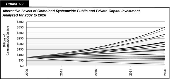
Exhibit 7-5 shows that current spending levels would be more than adequate to maintain average user costs in 2026 at 2006 levels, due to projected improvements in vehicle fuel economy. If capital spending on the types of improvements modeled in HERS were increased at an annual rate of approximately 3.21 percent in constant dollar terms, and this increased investment were financed by non-user sources, then it would be possible to reduce average user costs by 2.5 percent (therefore maintaining adjusted user costs at their base year level). If a fixed rate user charge financing mechanism were used instead, then in order to maintain adjusted user costs (equivalent to a 2.5 percent reduction in highway user costs), combined public and private highway capital investment would need to increase at an annual rate of 3.07 percent in constant dollar terms.
If variable rate user charges were instituted on all congested highway sections, then 2006 spending levels are projected to be more than adequate to maintain either average user costs or adjusted average user costs at their 2006 levels. A decrease in spending at an annual rate of approximately 1.37 percent in constant dollar terms would still allow adjusted average user costs to be maintained (equivalent to a 2.5 percent reduction in highway user costs), while an annual decrease of 7.64 percent would still be adequate to maintain average user costs.
Exhibit 7-5 also shows that for any given funding level, average highway user costs (excluding taxes) will be lower when a variable rate user charge is imposed than when fixed rate user charges or non-user sources serve as the funding mechanism. Charging highway users to finance highway investments in general, and charging peak period users to pay for the societal costs associated with peak period highway use in particular, allows the highway system to operate in a more efficient and rational manner from an economic perspective. For example, if combined public and private investment levels were sustained at 2006 levels, HERS projects that average user costs would decrease by 3.1 percent over 20 years if variable rate user charges were employed as a financial mechanism. In contrast, average user costs would decline by only 0.5 percent over 20 years if either fixed rate user charges or non-user sources were employed.
Assuming variable rate user charges were imposed, an annual increase of 4.55 percent over 2006 levels could result in a 5.1 percent decrease in average highway user costs in 2026 relative to 2006. This would translate into annual user costs savings of approximately $202 billion, based on projected future VMT at that level of investment. HERS projects that this is the greatest amount of user costs savings that can be achieved; additional investments beyond this point would not be cost-beneficial. In other words, this level of investment would be adequate to support all potential investments whose discounted stream of future benefits were equal to or exceeded their construction costs, which is mathematically represented by a benefit-cost ratio of 1.0 or higher. The benefit-cost ratios associated with each of the alternative levels of investment presented in Exhibit 7-5 for each funding mechanism are identified later in this chapter.
To a certain extent, additional investment in highway capacity expansion can serve as a partial substitute for the economically efficient pricing of highway facilities, and achieve some reduction in highway user costs. Constant dollar spending could grow at an average rate of 7.45 percent assuming a fixed rate user charge mechanism, or 7.76 percent assuming a non-user based financing mechanism, while still being invested in a cost-beneficial manner. However, as shown in Exhibit 7-5, despite these sharply higher levels of capital investment, neither of these financing mechanisms could reduce average user costs appreciably more than the reduction cited above as achievable at a much lower cost in conjunction with the application of congestion pricing (i.e., variable rate user charges).
Exhibit 7-5 also demonstrates that the performance impacts of financing through non-user sources are not significantly different than those projected for fixed-rate user based financing. These differences become larger as the level of highway investment increases beyond the current spending level because the imposition of fixed rate surcharges to support higher investment levels would offset a portion of the increased VMT that might otherwise occur. Conversely, if spending were to fall below current levels in constant dollar terms, the relative increase in user costs would be higher assuming that the savings were refunded to highway users in the form of lower highway user charges, which would tend to offset some of the reduction in VMT that might otherwise occur.
Projected VMT in 2026
Exhibit 7-6 identifies the projected VMT in 2026 for alternative investment levels and funding mechanisms. The values shown for HERS-modeled roads excludes VMT on functional classes for which HPMS sample data are not available (rural minor collector, rural local, and urban local). The estimated values for all roads were computed by applying the 20-year growth in VMT for HERS-modeled roads to total VMT on all roads in 2006. The projected VMT for all funding mechanisms identified in Exhibit 7-6 are influenced by the changes in user costs identified in Exhibit 7-5. The projected VMT assuming fixed rate user financing are also affected by the fixed charges identified in Exhibit 7-3, while the projected VMT assuming variable rate user financing are affected by both the variable and fixed charges identified in Exhibit 7-4.
| Annual Percent Change Relative to 2006 | Average Annual Capital Investment (Billions of 2006 Dollars) 1 Total Capital Outlay |
Average Annual Capital Investment (Billions of 2006 Dollars) 1 Spending Modeled in HERS |
Projected VMT in 2026 (Trillions of VMT) On HERS-Modeled Roads Funding Mechanism 2 Non-User Sources |
Projected VMT in 2026 (Trillions of VMT) On HERS-Modeled Roads Funding Mechanism 2 Fixed Rate User Charges |
Projected VMT in 2026 (Trillions of VMT) On HERS-Modeled Roads Funding Mechanism 2 Variable Rate User Charges |
Projected VMT in 2026 (Trillions of VMT) Estimated on All Roads Funding Mechanism 2 Non-User Sources |
Projected VMT in 2026 (Trillions of VMT) Estimated on All Roads Funding Mechanism 2 Fixed Rate User Charges |
Projected VMT in 2026 (Trillions of VMT) Estimated on All Roads Funding Mechanism 2 Variable Rate User Charges |
|---|---|---|---|---|---|---|---|---|
| 7.76% | $188.9 | $115.7 | 3.762 | 4.456 | ||||
| 7.45% | $182.0 | $111.5 | 3.758 | 3.662 | 4.452 | 4.338 | ||
| 6.70% | $166.5 | $102.0 | 3.749 | 3.669 | 4.442 | 4.347 | ||
| 6.41% | $160.9 | $98.6 | 3.746 | 3.671 | 4.437 | 4.349 | ||
| 5.25% | $140.6 | $86.1 | 3.733 | 3.678 | 4.422 | 4.357 | ||
| 5.15% | $139.0 | $85.1 | 3.732 | 3.678 | 4.421 | 4.357 | ||
| 5.03% | $137.1 | $84.0 | 3.731 | 3.679 | 4.419 | 4.358 | ||
| 4.65% | $131.2 | $80.4 | 3.726 | 3.679 | 4.414 | 4.359 | ||
| 4.55% | $129.7 | $79.5 | 3.725 | 3.680 | 3.596 | 4.413 | 4.359 | 4.260 |
| 4.17% | $124.2 | $76.1 | 3.721 | 3.680 | 3.596 | 4.407 | 4.360 | 4.260 |
| 3.30% | $112.6 | $69.0 | 3.710 | 3.681 | 3.594 | 4.396 | 4.360 | 4.258 |
| 3.21% | $111.5 | $68.3 | 3.709 | 3.681 | 3.594 | 4.394 | 4.360 | 4.257 |
| 3.07% | $109.7 | $67.2 | 3.708 | 3.681 | 3.594 | 4.392 | 4.360 | 4.257 |
| 2.96% | $108.4 | $66.4 | 3.706 | 3.680 | 3.593 | 4.391 | 4.360 | 4.257 |
| 2.93% | $108.0 | $66.2 | 3.706 | 3.680 | 3.593 | 4.390 | 4.360 | 4.257 |
| 1.67% | $94.0 | $57.6 | 3.692 | 3.679 | 3.588 | 4.374 | 4.358 | 4.251 |
| 0.83% | $85.9 | $52.6 | 3.683 | 3.677 | 3.584 | 4.363 | 4.356 | 4.246 |
| 0.34% | $81.5 | $50.0 | 3.678 | 3.675 | 3.582 | 4.357 | 4.354 | 4.243 |
| 0.00% | $78.7 | $48.2 | 3.674 | 3.674 | 3.579 | 4.352 | 4.352 | 4.240 |
| -0.78% | $72.5 | $44.4 | 3.666 | 3.671 | 3.575 | 4.343 | 4.349 | 4.235 |
| -0.86% | $71.9 | $44.1 | 3.665 | 3.671 | 3.574 | 4.342 | 4.349 | 4.234 |
| -1.37% | $68.3 | $41.8 | 3.660 | 3.669 | 3.572 | 4.335 | 4.346 | 4.231 |
| -4.95% | $48.2 | $29.5 | 3.624 | 3.648 | 3.550 | 4.293 | 4.322 | 4.205 |
| -7.64% | $37.9 | $23.2 | 3.602 | 3.633 | 3.534 | 4.267 | 4.304 | 4.187 |
Exhibit 7-6 shows that if current spending levels were sustained in constant dollar terms, then projected VMT for HERS-modeled roads would rise from 2.561 trillion in 2006 to 3.674 trillion by 2026 assuming financing by either non-user sources or by fixed rate user charges, since the fixed rate charge in this instance would be zero. Assuming that the imposition of variable rate user charges offset by reductions to existing fixed rate user charges would slow the growth in VMT, the projected level in 2026 would be only 3.579 trillion. Similarly, if spending were to grow by 4.55 percent per year in constant dollar terms, projected VMT would be 3.680 trillion assuming fixed rate user financing compared to 3.596 assuming variable rate user financing. These differences occur because traveling at off-peak is not a perfect substitute for peak period travel, and more individuals would be likely to eliminate trips or seek out alternative modes of travel in response to a targeted peak period variable highway user charge than would be the case for a more broadly imposed fixed user charge. The transit section of Chapter 8 includes some analysis of the potential impacts that variable rate highway user charges could have on future transit travel growth and on the operational performance of transit systems. The implications of projected future growth rates are discussed in more detail in Chapter 9.
| Why do the projected VMT values assuming financing through fixed rate user charges start to decline after investment levels reach a certain point? | |
|
The decline in projected VMT for investment assuming fixed rate user financing begins to decline after projected investment rises past an annual growth rate of approximately 3.3 percent. This occurs because, as noted above, the VMT charge assumed by HERS is applied to only the VMT on HERS modeled roads, but was set at a level adequate to support higher funding for all types of capital investment, not just spending modeled in HERS. At a certain point, this charge has a deterrent effect on VMT growth that is stronger than the positive effect on such growth caused by declines in average highway user costs associated with improved conditions and performance.
Had the VMT charge been applied more broadly in this analysis, this decline would be smaller, or would not occur.
|
|
User Cost Components
Travel time costs constitute approximately 48.7 percent of the HERS baseline estimate of highway user costs in 2006 of $1.0980 per mile. Vehicle operating costs constitute approximately 35.0 percent of total user costs, while crash-related costs (which are reflected in vehicle insurance costs and other social costs) make up the remaining 16.3 percent. Exhibit 7-7 describes how travel time costs and vehicle operating costs are influenced by the total amount invested in highways, and the financing mechanisms employed to support such investment.
| Annual Percent Change Relative to 2006 | Average Annual Capital Investment (Billions of 2006 Dollars) 1 Total Capital Outlay |
Average Annual Capital Investment (Billions of 2006 Dollars) 1 Spending Modeled in HERS |
Percent Change in Average User Costs on Roads Modeled in HERS Travel Time Costs Funding Mechanism 3 Non-User Sources |
Percent Change in Average User Costs on Roads Modeled in HERS Travel Time Costs Funding Mechanism 3 Fixed Rate User Charges |
Percent Change in Average User Costs on Roads Modeled in HERS Travel Time Costs Funding Mechanism 3 Variable Rate User Charges |
Percent Change in Average User Costs on Roads Modeled in HERS Vehicle Operating Costs 2 Funding Mechanism 3 Non-User Sources |
Percent Change in Average User Costs on Roads Modeled in HERS Vehicle Operating Costs 2 Funding Mechanism 3 Fixed Rate User Charges |
Percent Change in Average User Costs on Roads Modeled in HERS Vehicle Operating Costs 2 Funding Mechanism 3 Variable Rate User Charges |
|---|---|---|---|---|---|---|---|---|
| 7.76% | $188.9 | $115.7 | -3.4% | -10.3% | ||||
| 7.45% | $182.0 | $111.5 | -3.2% | -3.8% | -10.1% | -10.0% | ||
| 6.70% | $166.5 | $102.0 | -2.6% | -3.2% | -9.8% | -9.6% | ||
| 6.41% | $160.9 | $98.6 | -2.4% | -2.9% | -9.6% | -9.5% | ||
| 5.25% | $140.6 | $86.1 | -1.4% | -1.9% | -9.0% | -8.9% | ||
| 5.15% | $139.0 | $85.1 | -1.4% | -1.8% | -8.9% | -8.9% | ||
| 5.03% | $137.1 | $84.0 | -1.3% | -1.7% | -8.9% | -8.8% | ||
| 4.65% | $131.2 | $80.4 | -1.0% | -1.4% | -8.7% | -8.6% | ||
| 4.55% | $129.7 | $79.5 | -0.9% | -1.3% | -3.9% | -8.6% | -8.5% | -9.5% |
| 4.17% | $124.2 | $76.1 | -0.6% | -0.9% | -3.7% | -8.4% | -8.3% | -9.3% |
| 3.30% | $112.6 | $69.0 | 0.1% | -0.1% | -3.3% | -7.9% | -7.8% | -8.9% |
| 3.21% | $111.5 | $68.3 | 0.2% | -0.1% | -3.3% | -7.8% | -7.8% | -8.9% |
| 3.07% | $109.7 | $67.2 | 0.3% | 0.1% | -3.2% | -7.8% | -7.7% | -8.8% |
| 2.96% | $108.4 | $66.4 | 0.4% | 0.2% | -3.2% | -7.7% | -7.6% | -8.8% |
| 2.93% | $108.0 | $66.2 | 0.5% | 0.2% | -3.1% | -7.7% | -7.6% | -8.7% |
| 1.67% | $94.0 | $57.6 | 1.4% | 1.3% | -2.5% | -6.8% | -6.8% | -8.1% |
| 0.83% | $85.9 | $52.6 | 2.1% | 2.0% | -2.1% | -6.3% | -6.3% | -7.7% |
| 0.34% | $81.5 | $50.0 | 2.4% | 2.4% | -1.8% | -6.0% | -6.0% | -7.4% |
| 0.00% | $78.7 | $48.2 | 2.7% | 2.7% | -1.7% | -5.8% | -5.8% | -7.2% |
| -0.78% | $72.5 | $44.4 | 3.4% | 3.5% | -1.3% | -5.5% | -5.4% | -6.8% |
| -0.86% | $71.9 | $44.1 | 3.5% | 3.6% | -1.3% | -5.4% | -5.4% | -6.8% |
| -1.37% | $68.3 | $41.8 | 3.9% | 4.0% | -1.0% | -5.1% | -5.1% | -6.5% |
| -4.95% | $48.2 | $29.5 | 6.7% | 7.0% | 0.6% | -3.3% | -3.2% | -4.7% |
| -7.64% | $37.9 | $23.2 | 8.6% | 9.0% | 1.7% | -2.2% | -2.2% | -3.4% |
Exhibit 7-7 indicates that vehicle operating costs are expected to decline at all levels of investment, regardless of which financing mechanism is used. As described earlier, the HERS analyses for this report incorporated EIA's forecasts of sharp increases in future fuel efficiency for the vehicle fleet as a result of changes in CAFE standard and other factors.
Exhibit 7-7 shows that the imposition of variable rate user charges to combat congestion would facilitate greater reductions in average user costs than could be achieved if other funding mechanisms were employed, even at much higher levels of investment. For example, if investment were to increase at an annual rate of 4.55 percent in constant dollar terms, and variable rate user charges were imposed, HERS projects that a 3.9 percent reduction in average travel time costs could be achieved. This reduction is more significant than it appears, since a significant portion of travel time costs include the fixed amount of time required to move from one point to another at free-flow speeds, and thus would not be affected by actions that reduce congestion. HERS projects that the best that could be achieved in terms of travel time savings assuming funding by fixed rate user charges would be a 3.8 percent reduction if investment were to increase at an average annual rate of 7.45 percent.
Exhibit 7-7 also shows that variable rate user charges have the potential to partially mitigate the potential impacts of reductions in highway investment on travel time costs. For example, if combined public and private capital investment in highways were to decline by 7.64 percent annually in constant dollar terms, HERS projects a 1.7 percent increase in average travel time costs assuming a variable rate user charge financing mechanism, compared to an 9.0 percent increase assuming fixed rate user financing.
The HPMS database does not contain location-specific information on crashes, or the presence or absence of safety devices such as guard rails or rumble strips. Consequently, the HERS analysis does not identify specific safety-oriented investment opportunities, but instead considers the ancillary safety impacts of capital investments that are directed primarily toward system rehabilitation or capacity expansion. As a result, the overall crash costs calculated by HERS do not vary as significantly at different investment levels as do travel time costs and vehicle operating costs. The HERS analysis projects small increases in crash costs in constant dollars over time, ranging from 0.1 percent at higher levels of investment to 2.4 percent if capital investment is significantly reduced. The analysis suggests that the imposition of variable rate congestion charges may have some minor safety implications as it facilitates higher speeds, which tends to increase crash severity.
Impact of Future Investment on Highway Operational Performance
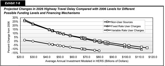
Exhibit 7-8 shows how average delay per VMT is influenced by the total amount invested in highways, and the financing mechanisms employed to support such investment. HERS estimates that if combined public and private highway capital investment were to increase by 4.65 percent annually in constant dollar terms and this increase were funded from non-user sources, then average delay per VMT in 2026 could be maintained at 2006 levels. If fixed rate user charges were employed instead, average delay per VMT could be maintained if capital investment grew by 4.17 percent annually in constant dollar terms; the difference is caused by the impact that the imposition of the fixed rate user charges would have on travel behavior. If current funding levels were sustained in constant dollar terms, it is projected that average delay per VMT would increase by 11.0 percent assuming funding from non-user sources.
| Annual Percent Change Relative to 2006 | Average Annual Investment (Billions of $2006) Total Capital Outlay |
Average Annual Investment (Billions of $2006) Spending Modeled in HERS |
Average Annual Investment (Billions of $2006) HERS System Expansion 2 Funding Mechanism Non-User Sources |
Average Annual Investment (Billions of $2006) HERS System Expansion 2 Funding Mechanism Fixed Rate User Charges |
Average Annual Investment (Billions of $2006) HERS System Expansion 2 Funding Mechanism Variable Rate User Charges |
Percent Change in Average Delay Per VMT on Roads Modeled in HERS Funding Mechanism Non-User Sources |
Percent Change in Average Delay Per VMT on Roads Modeled in HERS Funding Mechanism Fixed Rate User Charges |
Percent Change in Average Delay Per VMT on Roads Modeled in HERS Funding Mechanism Variable Rate User Charges |
|---|---|---|---|---|---|---|---|---|
| 7.76% | $188.9 | $115.7 | $64.3 | -8.5% | ||||
| 7.45% | $182.0 | $111.5 | $61.6 | $61.3 | -7.6% | -10.2% | ||
| 6.70% | $166.5 | $102.0 | $55.8 | $55.5 | -5.5% | -7.8% | ||
| 6.41% | $160.9 | $98.6 | $53.6 | $53.2 | -4.7% | -6.9% | ||
| 5.25% | $140.6 | $86.1 | $45.9 | $45.5 | -1.6% | -3.4% | ||
| 5.15% | $139.0 | $85.1 | $45.3 | $44.8 | -1.3% | -3.0% | ||
| 5.03% | $137.1 | $84.0 | $44.6 | $44.2 | -0.9% | -2.7% | ||
| 4.65% | $131.2 | $80.4 | $42.4 | $42.2 | 0.0% | -1.5% | ||
| 4.55% | $129.7 | $79.5 | $41.8 | $41.6 | $33.3 | 0.4% | -1.1% | -12.3% |
| 4.17% | $124.2 | $76.1 | $39.7 | $39.5 | $31.4 | 1.3% | 0.0% | -11.6% |
| 3.30% | $112.6 | $69.0 | $35.3 | $35.2 | $27.8 | 3.8% | 2.9% | -10.3% |
| 3.21% | $111.5 | $68.3 | $34.9 | $34.8 | $27.4 | 4.0% | 3.2% | -10.2% |
| 3.07% | $109.7 | $67.2 | $34.2 | $34.0 | $26.8 | 4.4% | 3.6% | -9.9% |
| 2.96% | $108.4 | $66.4 | $33.7 | $33.5 | $26.3 | 4.6% | 3.8% | -9.8% |
| 2.93% | $108.0 | $66.2 | $33.6 | $33.4 | $26.2 | 4.7% | 3.9% | -9.8% |
| 1.67% | $94.0 | $57.6 | $28.9 | $28.9 | $21.9 | 7.4% | 7.0% | -7.7% |
| 0.83% | $85.9 | $52.6 | $26.3 | $26.2 | $19.7 | 9.2% | 9.1% | -6.5% |
| 0.34% | $81.5 | $50.0 | $24.7 | $24.6 | $18.4 | 10.2% | 10.3% | -5.8% |
| 0.00% | $78.7 | $48.2 | $23.8 | $23.7 | $17.6 | 11.0% | 11.1% | -5.3% |
| -0.78% | $72.5 | $44.4 | $21.5 | $21.5 | $16.0 | 13.2% | 13.5% | -4.4% |
| -0.86% | $71.9 | $44.1 | $21.3 | $21.3 | $15.8 | 13.4% | 13.7% | -4.3% |
| -1.37% | $68.3 | $41.8 | $20.0 | $20.0 | $14.8 | 14.6% | 15.1% | -3.7% |
| -4.95% | $48.2 | $29.5 | $13.8 | $13.9 | $9.6 | 21.6% | 22.6% | 0.0% |
| -7.64% | $37.9 | $23.2 | $10.5 | $10.5 | $7.1 | 26.0% | 27.5% | 1.4% |
Assuming variable rate congestion charges were imposed broadly, HERS projects that current levels of highway capital investment would be adequate to reduce average delay per VMT, and that maintaining average delay at 2006 levels might still be achievable even if capital investment were to drop by 4.95 percent annually in constant dollar terms. If combined public and private highway capital investment were to rise by 4.55 percent annually in constant dollar terms, a 12.3 percent reduction in average delay per VMT could be achieved. HERS projects that such a reduction could not be achieved in the absence of such variable rate charges, even at much higher investment levels.
Exhibit 7-8 also identifies the portion of the spending modeled in HERS that was directed towards system expansion for each of the alternative investment levels that were analyzed. This is significant because investments in system expansion, such as the widening of existing highways or building new routes in existing corridors, would have a greater impact on delay than would investments in system rehabilitation such as the reconstruction or resurfacing of lanes on existing facilities.
If variable rate user charges were broadly imposed, this would significantly reduce congestion, thus reducing the potential benefits that could be achieved by widening existing highway sections. Consequently, the benefit-cost ratios associated with widening projects would tend to be lower, making it more likely that pavement reconstruction or resurfacing projects would be selected in a constrained funding environment. For example, if combined public and private highway capital investment were to rise by 4.55 percent annually in constant dollar terms, HERS would recommend that an average annual level of $41.8 billion be directed to system expansion assuming the additional funding comes from non-user sources, $41.6 billion assuming funding from fixed rate user charges, and $33.3 billion assuming variable rate user charges are imposed broadly. All of these amounts exceed current investment in system expansion by all levels of government combined, indicating that there are significant opportunities for cost-beneficial investment to add capacity to the highway system, regardless of which funding mechanism is employed.
Congestion Delay and Incident Delay
Exhibit 7-9 identifies the potential impacts of alternative investment levels and financing mechanisms on the congestion delay and incident delay components of the average delay per VMT figures presented in Exhibit 7-8. As noted above, the HERS model assumes the continuation of existing trends in the deployment of certain types of ITS and various operations strategies, which are expected to have a greater impact on reducing delay associated with isolated incidents than with delay associated with recurring congestion. Exhibit 7-9 shows that such deployments would be particularly effective in conjunction with the application of variable rate user charges, allowing reductions in average incident delay per VMT even at significantly reduced levels of highway capital investment. At current funding levels, HERS projects that incident delay would rise, but projects that an annual increase in combined public and private highway capital investment of between 0.83 percent to 1.67 percent in constant dollar terms may be sufficient to maintain incident delay at base year levels. At higher levels of investment, HERS projects that reductions in incident delay of 29.7 to 36.6 percent could be achieved, depending on the funding mechanism used to support this increased investment. Appendix A provides more details on the operations strategies and ITS considered in HERS, and Chapter 10 includes some analysis of the potential impacts of more aggressive deployment patterns than were assumed in the baseline analyses reflected in this chapter.
| Annual Percent Change Relative to 2006 | Average Annual Capital Investment (Billions of 2006 Dollars) 1 Total Capital Outlay |
Average Annual Capital Investment (Billions of 2006 Dollars) 1 Spending Modeled in HERS |
Percent Change in Delay on Roads Modeled in HERS Congestion Delay per VMT Funding Mechanism 2 Non-User Sources |
Percent Change in Delay on Roads Modeled in HERS Congestion Delay per VMT Funding Mechanism 2 Fixed Rate User Charges |
Percent Change in Delay on Roads Modeled in HERS Congestion Delay per VMT Funding Mechanism 2 Variable Rate User Charges |
Percent Change in Delay on Roads Modeled in HERS Incident Delay per VMT Funding Mechanism 2 Non-User Sources |
Percent Change in Delay on Roads Modeled in HERS Incident Delay per VMT Funding Mechanism 2 Fixed Rate User Charges |
Percent Change in Delay on Roads Modeled in HERS Incident Delay per VMT Funding Mechanism 2 Variable Rate User Charges |
|---|---|---|---|---|---|---|---|---|
| 7.76% | $188.9 | $115.7 | -1.8% | -29.7% | ||||
| 7.45% | $182.0 | $111.5 | -4.6% | -28.3% | -33.1% | |||
| 6.70% | $166.5 | $102.0 | -24.9% | -29.2% | ||||
| 6.41% | $160.9 | $98.6 | 4.3% | -23.7% | -27.5% | |||
| 5.25% | $140.6 | $86.1 | 8.8% | 5.8% | -17.5% | -20.8% | ||
| 5.15% | $139.0 | $85.1 | 9.3% | 6.5% | -17.0% | -20.0% | ||
| 5.03% | $137.1 | $84.0 | 9.8% | 6.9% | -16.4% | -19.4% | ||
| 4.65% | $131.2 | $80.4 | 11.2% | 8.8% | -14.6% | -17.1% | ||
| 4.55% | $129.7 | $79.5 | 11.8% | 9.4% | -8.3% | -14.1% | -16.7% | -36.6% |
| 4.17% | $124.2 | $76.1 | 13.3% | 11.1% | -7.3% | -12.7% | -14.9% | -35.4% |
| 3.30% | $112.6 | $69.0 | 17.1% | 15.5% | -5.4% | -8.2% | -9.4% | -32.7% |
| 3.21% | $111.5 | $68.3 | 17.5% | 15.9% | -5.2% | -8.0% | -9.1% | -32.5% |
| 3.07% | $109.7 | $67.2 | 18.1% | 16.7% | -4.8% | -7.4% | -8.6% | -32.2% |
| 2.96% | $108.4 | $66.4 | 18.4% | 17.0% | -4.6% | -6.9% | -8.1% | -31.9% |
| 2.93% | $108.0 | $66.2 | 18.5% | 17.1% | -4.5% | -6.8% | -8.0% | -31.8% |
| 1.67% | $94.0 | $57.6 | 22.8% | 22.1% | -1.6% | -27.8% | ||
| 0.83% | $85.9 | $52.6 | 25.6% | 25.4% | 0.0% | -25.4% | ||
| 0.34% | $81.5 | $50.0 | 27.2% | 27.3% | 1.1% | 2.8% | 2.8% | -23.8% |
| 0.00% | $78.7 | $48.2 | 28.4% | 28.6% | 1.8% | 4.0% | 4.2% | -22.6% |
| -0.78% | $72.5 | $44.4 | 31.7% | 32.2% | 3.0% | 8.2% | 8.7% | -20.5% |
| -0.86% | $71.9 | $44.1 | 32.0% | 32.5% | 3.2% | 8.6% | 9.1% | -20.3% |
| -1.37% | $68.3 | $41.8 | 33.9% | 34.6% | 4.0% | 10.6% | 11.4% | -19.0% |
| -4.95% | $48.2 | $29.5 | 44.1% | 45.9% | 8.9% | 23.3% | 24.9% | -10.7% |
| -7.64% | $37.9 | $23.2 | 50.4% | 53.0% | 10.7% | 32.0% | 34.1% | -7.7% |
Exhibit 7-9 also indicates that average delay per VMT due to recurring congestion is projected to rise by 1.8 percent if current spending is sustained over time in constant dollar terms and assuming that variable rate user charges are imposed, or by 28.6 percent assuming funding from fixed rate user charges. HERS projects that a 0.83 percent annual increase in combined public and private highway capital investment in constant dollar terms could be sufficient to maintain average congestion delay per VMT if variable rate congestion charges are imposed. If financing from non-user sources is employed, an annual constant dollar increase of 6.70 percent to 7.45 percent could be sufficient to maintain congestion delay. If fixed rate user charges are utilized, an annual increase of 6.41 percent to 6.70 percent in constant dollar terms might achieve this target.
Volume/Service Flow
Exhibit 7-10 shows how the estimated percentage of VMT occurring on roads with peak ratios of volume to service flow (V/SF) above 0.80 and 0.95 could be affected by alternative investment levels and funding mechanisms. As indicated in Chapter 4, these levels are generally used to describe congested and severely congested operating conditions on highways, respectively. If 2006 highway spending levels were maintained in constant dollar terms through 2026 in constant dollar terms, HERS projects that the percentage of VMT occurring on severely congested roads would increase from 13.0 percent in 2006 to 15.7 percent by 2026 if variable rate user charges are applied or to 21.2 percent by 2026 if other financing mechanisms are utilized.
| Annual Percent Change Relative to 2006 | Average Annual Capital Investment (Billions of 2006 Dollars) 1 Total Capital Outlay |
Average Annual Capital Investment (Billions of 2006 Dollars) 1 Spending Modeled in HERS |
Percent of VMT on Roads Modeled in HERS with V/SF > 0.80 Funding Mechanism 2 Non-User Sources |
Percent of VMT on Roads Modeled in HERS with V/SF > 0.80 Funding Mechanism 2 Fixed Rate User Charges |
Percent of VMT on Roads Modeled in HERS with V/SF > 0.80 Funding Mechanism 2 Variable Rate User Charges |
Percent of VMT on Roads Modeled in HERS with V/SF > 0.95 Funding Mechanism 2 Non-User Sources |
Percent of VMT on Roads Modeled in HERS with V/SF > 0.95 Funding Mechanism 2 Fixed Rate User Charges |
Percent of VMT on Roads Modeled in HERS with V/SF > 0.95 Funding Mechanism 2 Variable Rate User Charges |
|---|---|---|---|---|---|---|---|---|
| 7.76% | $188.9 | $115.7 | 29.1% | 12.3% | ||||
| 7.45% | $182.0 | $111.5 | 29.6% | 28.0% | 11.5% | |||
| 6.70% | $166.5 | $102.0 | 30.8% | 29.4% | ||||
| 6.41% | $160.9 | $98.6 | 31.2% | 29.9% | 14.4% | |||
| 5.25% | $140.6 | $86.1 | 32.8% | 31.8% | 16.1% | 15.2% | ||
| 5.15% | $139.0 | $85.1 | 33.0% | 32.0% | 16.2% | 15.4% | ||
| 5.03% | $137.1 | $84.0 | 33.1% | 32.2% | 16.4% | 15.6% | ||
| 4.65% | $131.2 | $80.4 | 33.5% | 32.8% | 17.0% | 16.3% | ||
| 4.55% | $129.7 | $79.5 | 33.6% | 32.9% | 29.0% | 17.1% | 16.5% | 10.9% |
| 4.17% | $124.2 | $76.1 | 34.0% | 33.4% | 29.5% | 17.5% | 16.9% | 11.3% |
| 3.30% | $112.6 | $69.0 | 34.9% | 34.4% | 30.9% | 18.4% | 18.0% | 12.3% |
| 3.21% | $111.5 | $68.3 | 35.0% | 34.5% | 31.0% | 18.5% | 18.1% | 12.4% |
| 3.07% | $109.7 | $67.2 | 35.1% | 34.6% | 31.2% | 18.7% | 18.2% | 12.6% |
| 2.96% | $108.4 | $66.4 | 35.2% | 34.8% | 31.4% | 18.8% | 18.4% | 12.7% |
| 2.93% | $108.0 | $66.2 | 35.2% | 34.8% | 31.4% | 18.8% | 18.4% | |
| 1.67% | $94.0 | $57.6 | 36.2% | 36.0% | 33.0% | 19.7% | 19.6% | |
| 0.83% | $85.9 | $52.6 | 37.0% | 36.8% | 34.1% | 20.5% | 20.5% | 15.0% |
| 0.34% | $81.5 | $50.0 | 37.3% | 37.2% | 34.5% | 20.9% | 20.9% | 15.4% |
| 0.00% | $78.7 | $48.2 | 37.5% | 37.4% | 34.8% | 21.2% | 21.2% | 15.7% |
| -0.78% | $72.5 | $44.4 | 38.1% | 38.1% | 35.4% | 22.0% | 22.0% | 16.3% |
| -0.86% | $71.9 | $44.1 | 38.1% | 38.2% | 35.5% | 22.0% | 22.1% | 16.3% |
| -1.37% | $68.3 | $41.8 | 38.4% | 38.6% | 35.9% | 22.5% | 22.6% | 16.8% |
| -4.95% | $48.2 | $29.5 | 39.9% | 40.2% | 37.9% | 24.5% | 24.9% | 18.8% |
| -7.64% | $37.9 | $23.2 | 40.5% | 41.0% | 38.8% | 25.5% | 26.1% | 19.6% |
| 2006 Baseline Values: | 23.6% | 23.6% | 23.6% | 13.0% | 13.0% | 13.0% | ||
HERS projects that an increase in combined public and private highway capital investment of 1.67 percent to 2.93 percent annually in constant dollar terms may be sufficient to maintain the percentage of VMT on severely congested roads at the 2006 levels if variable rate user charges are applied. If funding from fixed user charges is employed, an annual constant dollar increase of 6.41 percent to 6.70 percent could be sufficient to achieve this target; if funding from non-user sources is utilized, an annual increase of 6.70 percent to 7.45 percent in constant dollar terms might be needed to achieve the same level of performance.
Exhibit 7-10 also indicates that if combined public and private highway capital investment were sustained at 2006 levels, the percentage of VMT on congested roads would be projected to increase from 23.6 percent to somewhere between 34.8 percent and 37.5 percent in 2026, depending on the funding mechanism utilized to support this investment. It should be noted that the relative impacts of imposing variable rate user charges projected by HERS are greater for severely congested roads than for moderately congested roads, indicating that the widespread adoption of variable congestion charges would grow more effective as the degree of congestion on a facility increases in severity.
For a potential capacity improvement to be implemented as part of a HERS scenario, the improvement must meet the minimum benefit-cost ratio cutoff associated with the level of investment being analyzed. As a result, there may be some road segments in a given time period that meet or exceed the threshold for being considered congested, but that do not merit capacity expansion in HERS. Exhibit 7-10 suggests that it would not be cost-beneficial to maintain the percentage of VMT occurring on roads with V/SF ratios greater than 0.80 at the base year 2006 level, regardless of which funding mechanism is employed. This suggests that the existence of some limited degree of congestion may be desirable from an economic point of view in terms of regulating travel demand, and that significant capital expenditures to address congestion may only be warranted when congestion worsens in severity to a level beyond the 0.80 V/SF threshold.
| Why do the average speeds presented in Exhibit 7-11 appear relatively low? | |
|
The average speed of 42.7 miles per hour in 2006 represents a composite value for all of the roads modeled in HERS, which include a large number of urban collectors with speed limits of 25 miles per hour. HERS estimates the average speed on Interstate highways as 59.7 miles per hour.
Assuming variable rate user charges were imposed, and combined public and private highway capital investment were to increase by 4.55 percent per year through 2026 in constant dollar terms, HERS projects average Interstate speeds would rise to 66.1 miles per hour. Assuming fixed rate user financing, HERS projects that if spending were to increase by 7.45 percent per year through 2026, average Interstate speeds would rise to 65.1 miles per hour.
|
|
Speed
Exhibit 7-11 shows how average vehicle speeds could be affected by alternative investment levels and funding mechanisms. This measure corresponds to one of the main transit performance measures used in the Transit Economic Requirements Model, which is discussed later in this chapter.
| Annual Percent Change Relative to 2006 | Average Annual Capital Investment (Billions of 2006 Dollars) 1 Total Capital Outlay |
Average Annual Capital Investment (Billions of 2006 Dollars) 1 Spending Modeled in HERS |
Average Speed on Roads Modeled in HERS Funding Mechanism 2 Non-User Sources |
Average Speed on Roads Modeled in HERS Funding Mechanism 2 Fixed Rate User Charges |
Average Speed on Roads Modeled in HERS Funding Mechanism 2 Variable Rate User Charges |
|---|---|---|---|---|---|
| 7.76% | $188.9 | $115.7 | 43.9 | ||
| 7.45% | $182.0 | $111.5 | 43.8 | 44.1 | |
| 6.70% | $166.5 | $102.0 | 43.6 | 43.8 | |
| 6.41% | $160.9 | $98.6 | 43.5 | 43.7 | |
| 5.25% | $140.6 | $86.1 | 43.2 | 43.4 | |
| 5.15% | $139.0 | $85.1 | 43.2 | 43.3 | |
| 5.03% | $137.1 | $84.0 | 43.1 | 43.3 | |
| 4.65% | $131.2 | $80.4 | 43.0 | 43.2 | |
| 4.55% | $129.7 | $79.5 | 43.0 | 43.1 | 44.1 |
| 4.17% | $124.2 | $76.1 | 43.0 | 44.0 | |
| 3.30% | $112.6 | $69.0 | 43.8 | ||
| 3.21% | $111.5 | $68.3 | 42.6 | 43.8 | |
| 3.07% | $109.7 | $67.2 | 42.6 | 42.6 | 43.8 |
| 2.96% | $108.4 | $66.4 | 42.5 | 42.6 | 43.8 |
| 2.93% | $108.0 | $66.2 | 42.5 | 42.6 | 43.8 |
| 1.67% | $94.0 | $57.6 | 42.2 | 42.2 | 43.6 |
| 0.83% | $85.9 | $52.6 | 41.9 | 42.0 | 43.4 |
| 0.34% | $81.5 | $50.0 | 41.8 | 41.8 | 43.3 |
| 0.00% | $78.7 | $48.2 | 41.7 | 41.7 | 43.3 |
| -0.78% | $72.5 | $44.4 | 41.5 | 41.5 | 43.1 |
| -0.86% | $71.9 | $44.1 | 41.5 | 41.4 | 43.1 |
| -1.37% | $68.3 | $41.8 | 41.3 | 41.3 | |
| -4.95% | $48.2 | $29.5 | 40.4 | 40.3 | |
| -7.64% | $37.9 | $23.2 | 39.7 | 39.6 | 42.0 |
| 2006 Baseline Values: | 42.7 | 42.7 | 42.7 | ||
HERS projects that sustaining combined public and private highway capital level at 2006 levels in constant dollar terms would be sufficient to allow average speeds to increase above the baseline 2006 level of 42.7 miles per hour on roads modeled in HERS, if variable rate user charges were imposed. If funding from fixed user charges were employed, an annual constant dollar increase of 3.21 percent to 3.30 percent could be sufficient to achieve this target; if funding from non-user sources were utilized, an annual increase of 3.30 percent to 4.17 percent in constant dollar terms might be needed to achieve the same level of performance.
Impact of Future Investment on Highway Physical Conditions
Exhibit 7-12 shows how pavement ride quality (based on the International Roughness Index [IRI] defined in Chapter 3) is influenced by the total amount invested in highways, and the financing mechanisms employed to support such investment. HERS estimates that if combined public and private highway capital investment were to increase by 0.34 percent annually in constant dollar terms and this increase were funded from variable rate user charges, then average IRI in 2026 for roads modeled in HERS could be maintained at 2006 levels. If fixed rate user charges were employed instead, average ride quality could be maintained if capital investment grew by 2.93 percent annually in constant dollar terms; assuming funding from non-user sources, an annual growth rate of 2.96 percent annually would be required to achieve these targets. In comparing these figures, it is important to note that HERS directs a higher percentage of investment towards system rehabilitation for the analyses assuming variable rate user charges, as the broad imposition of such charges would significantly reduce congestion, thus reducing the potential benefits that could be achieved by widening existing highway sections. Consequently, the benefit-cost ratios associated with system expansion projects would tend to be lower, making it more likely that pavement reconstruction or resurfacing projects would be selected in a constrained funding environment, as shown in Exhibit 7-12. Although the addition of new, smooth lanes to the existing system would bring up average ride quality a little bit, investments in system rehabilitation would have a larger, more direct impact on this measure of pavement condition.
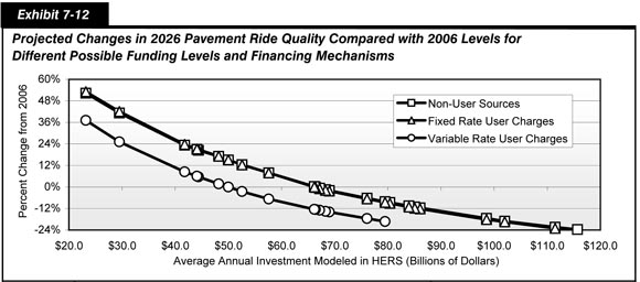
| Annual Percent Change Relative to 2006 | Average Annual Investment (Billions of $2006) Total Capital Outlay |
Average Annual Investment (Billions of $2006) Spending Modeled in HERS |
Average Annual Investment (Billions of $2006) HERS System Rehabiliation 2 Funding Mechanism Non-User Sources |
Average Annual Investment (Billions of $2006) HERS System Rehabiliation 2 Funding Mechanism Fixed Rate User Charges |
Average Annual Investment (Billions of $2006) HERS System Rehabiliation 2 Funding Mechanism Variable Rate User Charges |
Percent Change in Average IRI on Roads Modeled in HERS Funding Mechanism Non-User Sources |
Percent Change in Average IRI on Roads Modeled in HERS Funding Mechanism Fixed Rate User Charges |
Percent Change in Average IRI on Roads Modeled in HERS Funding Mechanism Variable Rate User Charges |
|---|---|---|---|---|---|---|---|---|
| 7.76% | $188.9 | $115.7 | $51.4 | -23.8% | ||||
| 7.45% | $182.0 | $111.5 | $50.0 | $50.2 | -22.4% | -23.1% | ||
| 6.70% | $166.5 | $102.0 | $46.2 | $46.5 | -19.1% | -19.4% | ||
| 6.41% | $160.9 | $98.6 | $45.0 | $45.4 | -17.5% | -18.1% | ||
| 5.25% | $140.6 | $86.1 | $40.2 | $40.6 | -11.7% | -12.2% | ||
| 5.15% | $139.0 | $85.1 | $39.8 | $40.3 | -11.1% | -11.8% | ||
| 5.03% | $137.1 | $84.0 | $39.4 | $39.7 | -10.5% | -11.2% | ||
| 4.65% | $131.2 | $80.4 | $38.0 | $38.2 | -8.7% | -9.1% | ||
| 4.55% | $129.7 | $79.5 | $37.7 | $37.9 | $46.2 | -8.2% | -8.6% | -19.3% |
| 4.17% | $124.2 | $76.1 | $36.4 | $36.6 | $44.7 | -6.3% | -6.6% | -17.6% |
| 3.30% | $112.6 | $69.0 | $33.6 | $33.7 | $41.2 | -1.9% | -2.3% | -14.0% |
| 3.21% | $111.5 | $68.3 | $33.4 | $33.5 | $40.9 | -1.5% | -1.9% | -13.6% |
| 3.07% | $109.7 | $67.2 | $33.1 | $33.2 | $40.5 | -0.7% | -1.0% | -13.0% |
| 2.96% | $108.4 | $66.4 | $32.7 | $32.9 | $40.1 | 0.0% | -0.2% | -12.5% |
| 2.93% | $108.0 | $66.2 | $32.6 | $32.8 | $40.0 | 0.3% | 0.0% | -12.5% |
| 1.67% | $94.0 | $57.6 | $28.7 | $28.8 | $35.7 | 7.9% | 7.9% | -6.7% |
| 0.83% | $85.9 | $52.6 | $26.4 | $26.5 | $33.0 | 12.5% | 12.4% | -2.6% |
| 0.34% | $81.5 | $50.0 | $25.2 | $25.3 | $31.5 | 15.0% | 15.1% | 0.0% |
| 0.00% | $78.7 | $48.2 | $24.5 | $24.5 | $30.6 | 17.0% | 17.1% | 1.8% |
| -0.78% | $72.5 | $44.4 | $23.0 | $23.0 | $28.5 | 20.4% | 20.8% | 5.7% |
| -0.86% | $71.9 | $44.1 | $22.8 | $22.8 | $28.3 | 20.8% | 21.2% | 6.0% |
| -1.37% | $68.3 | $41.8 | $21.8 | $21.8 | $27.1 | 23.3% | 23.8% | 8.4% |
| -4.95% | $48.2 | $29.5 | $15.7 | $15.6 | $19.9 | 41.3% | 42.0% | 25.2% |
| -7.64% | $37.9 | $23.2 | $12.7 | $12.7 | $16.0 | 52.3% | 53.1% | 37.1% |
If current investment levels were sustained for 20 years in constant dollar terms, HERS projects that average pavement roughness would increase by 17.1 percent relative to base year levels assuming funding from fixed rate user sources, compared to an increase of 1.8 percent if variable rate user charges were imposed. This difference is mainly the result of the larger relative investment in system rehabilitation recommended by HERS for all funding levels for analyses assuming the broad adoption of variable rate congestion charges. However, the lower levels of VMT associated with the variable rate user charges would have a minor impact on improving average IRI as well.
Exhibit 7-12 suggests that while more can be achieved at any given funding level in terms of improving pavement ride quality assuming the broad imposition of variable rate user charges, additional reductions in average pavement roughness could be achieved at significantly higher spending levels assuming funding from non-user sources or fixed rate user charges. If combined public and private highway capital investment were to increase by 7.76 percent assuming non-user financing, HERS projects a 23.8 percent reduction in average pavement roughness; this exceeds the 19.3 percent reduction that could be economically accommodated assuming a 4.55 percent annual increase in spending and the widespread adoption of variable rate user charges. This difference is attributable to the reduced number of widening actions taken by HERS for the analyses assuming the adoption of variable rate user charges. When HERS adds new lanes to an existing facility, as it is more likely to do if variable rate pricing is not in place, it also resurfaces or reconstructs all of the existing lanes. In some cases, these pavement improvements occur earlier in the life of the pavement than would normally be the case in the absence of the widening action, and would not have been cost-beneficial on their own. Consequently, the reduced number of widening actions taken by HERS under the variable rate funding analyses causes some of these pavement actions to be deferred beyond the 20-year period considered as part of this analysis, until such time as their relative benefits exceed their costs.
Exhibit 7-13 shows how the projected percentage of VMT on pavement with IRI values below 95 and 170 could be affected by alternative levels of investment and financing mechanisms. The pavement condition criteria presented in Chapter 3 defined these levels as the thresholds for rating pavement ride quality as good and acceptable, respectively.
| Annual Percent Change Relative to 2006 | Average Annual Capital Investment (Billions of 2006 Dollars) Total Capital Outlay |
Average Annual Capital Investment (Billions of 2006 Dollars) Spending Modeled in HERS |
Percent of VMT on Roads Modeled in HERS With IRI<95: Funding Mechanism 2 Non-User Sources |
Percent of VMT on Roads Modeled in HERS With IRI<95: Funding Mechanism 2 Fixed Rate User Charges |
Percent of VMT on Roads Modeled in HERS With IRI<95: Funding Mechanism 2 Variable Rate User Charges |
Percent of VMT on Roads Modeled in HERS With IRI<170 Funding Mechanism 2 Non-User Sources |
Percent of VMT on Roads Modeled in HERS With IRI<170 Funding Mechanism 2 Fixed Rate User Charges |
Percent of VMT on Roads Modeled in HERS With IRI<170 Funding Mechanism 2 Variable Rate User Charges |
|---|---|---|---|---|---|---|---|---|
| 7.76% | $188.9 | $115.7 | 74.6% | 91.2% | ||||
| 7.45% | $182.0 | $111.5 | 73.6% | 74.0% | 90.7% | 90.9% | ||
| 6.70% | $166.5 | $102.0 | 71.1% | 71.4% | 89.6% | 89.7% | ||
| 6.41% | $160.9 | $98.6 | 70.1% | 70.6% | 89.1% | 89.3% | ||
| 5.25% | $140.6 | $86.1 | 66.1% | 66.4% | 87.2% | 87.3% | ||
| 5.15% | $139.0 | $85.1 | 65.7% | 66.2% | 87.0% | 87.1% | ||
| 5.03% | $137.1 | $84.0 | 65.3% | 65.6% | 86.8% | 86.9% | ||
| 4.65% | $131.2 | $80.4 | 64.0% | 64.2% | 86.2% | 86.2% | ||
| 4.55% | $129.7 | $79.5 | 63.6% | 63.9% | 70.7% | 90.4% | ||
| 4.17% | $124.2 | $76.1 | 62.4% | 62.6% | 69.6% | 89.8% | ||
| 3.30% | $112.6 | $69.0 | 59.5% | 59.5% | 66.7% | 84.0% | 84.0% | 88.6% |
| 3.21% | $111.5 | $68.3 | 59.3% | 59.1% | 66.4% | 83.9% | 83.9% | 88.5% |
| 3.07% | $109.7 | $67.2 | 58.8% | 58.8% | 66.1% | 83.7% | 83.7% | 88.3% |
| 2.96% | $108.4 | $66.4 | 58.4% | 58.5% | 65.7% | 83.5% | 83.5% | 88.1% |
| 2.93% | $108.0 | $66.2 | 58.3% | 58.4% | 65.7% | 83.4% | 83.5% | 88.1% |
| 1.67% | $94.0 | $57.6 | 54.0% | 53.9% | 61.3% | 81.2% | 81.1% | |
| 0.83% | $85.9 | $52.6 | 51.3% | 51.3% | 58.2% | 79.7% | 79.7% | |
| 0.34% | $81.5 | $50.0 | 49.8% | 49.9% | 56.3% | 79.0% | 79.0% | 83.9% |
| 0.00% | $78.7 | $48.2 | 55.1% | 78.4% | 78.5% | 83.2% | ||
| -0.78% | $72.5 | $44.4 | 52.4% | 77.4% | 77.3% | 82.0% | ||
| -0.86% | $71.9 | $44.1 | 46.2% | 46.2% | 52.2% | 77.3% | 77.2% | 81.9% |
| -1.37% | $68.3 | $41.8 | 44.7% | 44.7% | 76.4% | 76.3% | 81.1% | |
| -4.95% | $48.2 | $29.5 | 36.6% | 36.5% | 71.9% | 71.7% | 75.9% | |
| -7.64% | $37.9 | $23.2 | 32.5% | 32.4% | 34.6% | 69.4% | 69.2% | 72.7% |
| 2006 Baseline Values: | 48.1% | 48.1% | 48.1% | 85.8% | 85.8% | 85.8% | ||
If 2006 highway spending levels were maintained through 2026 in constant dollar terms, HERS projects that the percentage of VMT occurring on pavements with good ride quality would increase from 48.1 percent in 2006 to 55.1 percent by 2026 if variable rate user charges are applied or to between 48.7 percent to 48.8 percent by 2026 if such charges are not applied. The difference is attributable primarily to the higher portion investment directed by HERS to system rehabilitation (i.e., pavement resurfacing or reconstruction) identified in Exhibit 7-12. HERS projects that the highest percentage of VMT on pavements with good ride quality that could be achieved through cost-beneficial investment would range from 70.7 percent to 74.6 percent, depending on the financing mechanism utilized. Traffic volumes on some of the roads modeled in HERS would not justify meeting this standard because the relative benefits to users resulting from this level of ride quality would be outweighed by the capital costs and work zone delays associated with the pavement actions that could achieve it.
Exhibit 7-13 also shows that if combined public and private highway capital investment were sustained at 2006 levels, the percentage of VMT occurring on roads with acceptable ride quality would be projected to decrease from 85.8 percent to between 78.4 percent and 83.2 percent in 2026, depending on the funding mechanism utilized to support this investment. HERS projects that an annual constant dollar increase in combined public and private highway capital investment of 0.83 percent to 1.67 percent could be sufficient to maintain the percentage of VMT on pavements with acceptable ride quality if congestion charges are imposed; if financing from non-user sources or fixed rate user charges is employed, an annual constant dollar increase of 4.17 percent to 4.55 percent might achieve this target. HERS projects that the highest percentage of VMT on pavements with acceptable ride quality that could be achieved through cost-beneficial investment would range from 90.4 percent to 91.2 percent, depending on the financing mechanism utilized. As noted in Chapter 3, the IRI threshold of 170 used to identify acceptable ride quality was originally set to measure performance on the NHS and may not fully reflect an acceptable standard for non-NHS routes, which tend to have lower travel volumes and speeds.
Benefit-Cost Ratios
As noted earlier, the benefits considered in HERS include reductions in highway user costs, agency costs and societal costs. The costs considered in HERS are the capital costs associated with a particular potential highway improvement. The HERS analysis presented in this report was performed by imposing a funding constraint on the model for investment in four consecutive 5-year analysis periods (for a total analysis period of 20 years). Under this type of analysis, HERS ranks potential improvements in order by their benefit-cost ratios and then implements them until the funding constraint is reached. Higher funding levels will thus include projects with lower benefit-cost ratios, both at the margin and on average. Appendix A contains a more detailed description of the project selection and implementation process used by HERS.
Exhibit 7-14 identifies benefit-cost ratio cutoff points associated with the alternative investment levels and funding levels analyzed. These values represent the benefit-cost ratio of the least attractive project that would be implemented at that level of investment. For example, if investment were to grow by 3.30 percent annually in constant dollar terms, and invested in order of potential projects' benefit-cost ratios as assumed by HERS, the lowest benefit-cost ratio for any project implemented is estimated to be 1.95 assuming funding from non-user sources, 1.93 assuming funding from fixed user sources, and 1.20 assuming funding from variable user sources. The lower benefit-cost ratio cutoffs associated with funding from fixed user or variable user sources are partially a function of the lower projected VMT levels identified in Exhibit 7-6; there would be fewer users to benefit from highway investments (in that some users would chose not to make low-value trips if they had to pay the real costs of such trips), and thus the level of potential highway user costs savings is lower for any given project. In addition, because the imposition of variable rate user charges on a highway section would tend to reduce peak period congestion levels and lead to significant travel time savings, the relative benefits that could be achieved by widening that highway section would be reduced.
| Annual Percent Change Relative to 2006 | Average Annual Investment (Billions of 2006 Dollars) Total Capital Outlay |
Average Annual Investment (Billions of 2006 Dollars) Spending Modeled in HERS1 |
Minimum Benefit-Cost Ratio 2 Funding Mechanism Non-User Sources |
Minimum Benefit-Cost Ratio 2 Funding Mechanism Fixed Rate User Charges |
Minimum Benefit-Cost Ratio 2 Funding Mechanism Variable Rate User Charges |
Funding Level Description 3 |
|---|---|---|---|---|---|---|
| 7.76% | $188.9 | $115.7 | 1.00 | Minimum BCR=1.0 (Non-User) | ||
| 7.45% | $182.0 | $111.5 | 1.06 | 1.00 | Minimum BCR=1.0 (Fixed User) | |
| 6.70% | $166.5 | $102.0 | 1.20 | 1.15 | Minimum BCR=1.2 (Non-User) | |
| 6.41% | $160.9 | $98.6 | 1.26 | 1.20 | Minimum BCR=1.2 (Fixed User) | |
| 5.25% | $140.6 | $86.1 | 1.50 | 1.45 | Minimum BCR=1.5 (Non-User) | |
| 5.15% | $139.0 | $85.1 | 1.53 | 1.46 | See NBIAS discussion | |
| 5.03% | $137.1 | $84.0 | 1.55 | 1.50 | Minimum BCR=1.5 (Fixed User) | |
| 4.65% | $131.2 | $80.4 | 1.63 | 1.59 | Maintain Average Delay (Non-User) | |
| 4.55% | $129.7 | $79.5 | 1.65 | 1.62 | 1.00 | Minimum BCR=1.0 (Variable User) |
| 4.17% | $124.2 | $76.1 | 1.74 | 1.71 | 1.06 | Maintain Average Delay (Fixed User) |
| 3.30% | $112.6 | $69.0 | 1.95 | 1.93 | 1.20 | Minimum BCR=1.2 (Variable User) |
| 3.21% | $111.5 | $68.3 | 1.97 | 1.96 | 1.21 | Maintain Adjusted User Cost (Non-User) |
| 3.07% | $109.7 | $67.2 | 2.01 | 1.98 | 1.24 | Maintain Adjusted User Cost (Fixed User) |
| 2.96% | $108.4 | $66.4 | 2.04 | 2.01 | 1.25 | Maintain Average IRI (Non-User) |
| 2.93% | $108.0 | $66.2 | 2.05 | 2.02 | 1.26 | Maintain Average IRI (Fixed User) |
| 1.67% | $94.0 | $57.6 | 2.42 | 2.42 | 1.50 | Minimum BCR=1.5 (Variable User) |
| 0.83% | $85.9 | $52.6 | 2.71 | 2.70 | 1.71 | See NBIAS discussion |
| 0.34% | $81.5 | $50.0 | 2.87 | 2.86 | 1.82 | Maintain Average IRI (Variable User) |
| 0.00% | $78.7 | $48.2 | 2.88 | 2.89 | 1.90 | Actual 2006 Capital Outlay |
| -0.78% | $72.5 | $44.4 | 2.94 | 2.94 | 2.12 | Maintain Average User Cost (Fixed User) |
| -0.86% | $71.9 | $44.1 | 2.94 | 2.95 | 2.14 | Maintain Average User Cost (Non-User) |
| -1.37% | $68.3 | $41.8 | 2.98 | 2.99 | 2.25 | Maintain Adjusted User Cost (Variable User) |
| -4.95% | $48.2 | $29.5 | 3.22 | 3.24 | 2.42 | Maintain Average Delay (Variable User) |
| -7.64% | $37.9 | $23.2 | 3.42 | 3.43 | 2.55 | Maintain Average User Cost (Variable User) |
It is important to note that the benefit-cost ratio cutoffs shown in Exhibit 7-14 represent the lowest value estimated by HERS at any point during the 20-year analysis period. At higher levels of investment, the cutoff points tend to fall over this period. For example, if investment were to grow by 4.55 percent annually in constant dollar terms, and assuming funding from variable rate user sources, HERS estimates that the benefit-cost ratio cutoff would be 1.99 in the first 5-year period, falling gradually to 1.00 in the fourth 5-year period. In contrast, at lower levels of investment, the opposite tendency would be true. For instance, if investment were to decrease from the 2006 level by 7.64 percent annually and assuming funding from non-user sources, HERS estimates that the benefit-cost ratio cutoff would be 3.42 in the first 5-year period, rising gradually to 6.16 in the fourth 5-year period.
The benefit-cost ratios identified in Exhibit 7-14 represent minimum values, and many projects implemented at each investment level would have much higher benefit-cost ratios. Consequently, the average benefit-cost ratio for each level of investment would be significantly higher. Assuming funding by non-user sources, the marginal benefit-cost ratios of 1.00 to 3.42 identified in Exhibit 7-14 would be associated with average benefit-cost ratios ranging from 2.84 to 7.56; if fixed rate user charges were utilized, the marginal benefit-cost ratios of 1.00 to 3.43 would correspond to average benefit-cost ratios ranging from 2.85 to 7.62, weighted by project cost. Assuming variable rate user charges were broadly adopted, the marginal benefit-cost ratios of 1.00 to 2.55 identified in Exhibit 7-14 would be associated with average benefit-cost ratios ranging from 2.75 to 6.19. In interpreting these figures, it should be noted that average benefit-cost ratios do not constitute a good indicator of the relative merits of one investment level versus another because they only capture the benefits associated with projects that are implemented, and do not reflect the disbenefits associated with projects that were not implemented. Hence, multiplying these average benefit-cost ratios by average spending would not yield an accurate measure of the net benefits associated with a particular investment level.
| What are some considerations that should be taken into account when interpreting the benefit-cost ratios presented in Exhibit 7-14? | |
|
The reader should use caution when considering the attractiveness of different funding mechanism and investment levels based only on the benefit-cost ratios. An attempt to select among funding mechanisms and investment levels by using the "highest" benefit-cost ratio in Exhibit 7-14 would almost certainly result in a misallocation of resources from an economic standpoint. In particular, although the incremental benefit-cost ratios for project investments under fixed rate user charges are higher than for project investments under variable rate user charges for any given funding level, the key parameter of interest for selecting the "best" economic package of investments and funding mechanisms would be the overall benefit to society attributable to the combined effects of both project investments and funding mechanisms. As shown in Exhibit 7-5 (see percent changes in "adjusted average user costs"), the greatest social benefit (as measured by the monetary value of total reductions in user costs) for any given funding level occurs when cost-beneficial investments are pursued in coordination with a variable rate funding mechanism.
Similarly, due to the multi-period analysis used in HERS to evaluate investments over a 20 year period, the reader should not attempt to multiply the benefit-cost ratios in Exhibit 7-14 by the associated total capital outlays to calculate the social benefits of that investment level. To do so would yield the false impression in some instances that higher investment levels yield lower total benefits. There are several reasons why this is so. First, the "Total Capital Outlay" figures in Exhibit 7-14 represent an average annual amount over 20 years whereas the benefit-cost ratio values reported in the exhibit represent the lowest such value among the four 5-year investment periods that constitute the 20-year analysis period. Unless benefit-cost ratio values are constant over the four investment periods, the application of the lowest benefit-cost ratio to the average annual funding would be misleading. More importantly, however, is the failure of this method to account for deferred (unrealized) benefits over the full 20-year analysis period. In the case of scenarios with declining annual funding levels, HERS will tend to defer all investments except those with very high benefit-cost ratios until later in the 20-year analysis period (if it captures them at all). Society would not enjoy the benefits of many strong investments until much later in the 20-year overall analysis period—benefits that society would realize more quickly in higher funding scenarios. In short, the cumulative value of the 20-year loss of benefits associated with deferring strong investments at low funding levels is not captured by the simple multiplication of a benefit-cost ratio by a 1-year average total capital outlay. Only a multi-year summary of benefits stretching over 20 years would yield a true picture of society's total benefits from a given investment level. This impact is best captured in changes to the "Average User Cost" values and other statistics reported in Exhibit 7-5 and Exhibits 7-7 through 7-13. Chapter 9 includes some additional discussion regarding the timing of investments. Finally, as noted above, the benefit-cost ratios for investments do not capture the benefits associated with the funding mechanism itself (e.g., fixed versus variable user charges).
|
|
The funding level descriptions shown in Exhibit 7-14 are included to identify the analytical significance of each of the alternative funding growth rates that are analyzed in this section. Some of these investment levels are associated with a particular minimum benefit-cost ratio; others are associated with maintaining particular indicators of conditions and performance as presented in previous exhibits. Two of these investment levels were selected due to their analytical significance in the NBIAS model, as will be discussed later in this section.
Due to the large number of potential highway investments analyzed in HERS, the minimum benefit-cost ratios identified in Exhibit 7-14 for alternative highway investment levels should be largely consistent with those for major system components. For example, if combined public and private investment in the types of capital improvements modeled in HERS were to increase by 1.67 percent annually and variable rate user charges were applied, the minimum BCR of 1.5 would generally apply to the portion of that investment directed to the NHS, and that portion directed to individual functional systems.
Impacts of NHS Investments Modeled by HERS
As described in Chapter 2, the NHS constitutes a critical subset of the total highway system, including the Interstate System as well as other routes most critical to national defense, mobility, and commerce. This section examines the total spending modeled in HERS, identifying the portion of this investment that is directed by the model to the NHS, and the impacts that such investment could have on future NHS conditions and performance.
Impact of Future Investment on NHS User Costs
Exhibit 7-15 describes how average total user costs and average adjusted user costs on the NHS are influenced by the total amount invested on the system, and the financing mechanisms utilized to support such investment. As discussed earlier in this chapter, the "Adjusted Average User Cost" figures offset the impacts of the improvements in future fuel efficiency assumed as part of the analysis, in order to provide a better measure of the impact that changes in system conditions and performance have on highway user costs. The first 24 investment levels described in Exhibit 7-15 correspond to the systemwide spending levels explored earlier in this chapter that are analytically significant in terms of systemwide investment impacts; the next row has been included to specifically identify the costs associated with maintaining adjusted average user costs for each of the three types of funding mechanisms, while the last row shows the impacts of sustaining investment on the NHS at 2006 levels in constant dollar terms for each funding mechanism.
| Annual Percent Change Relative to 2006 | Average Annual HERS-Modeled Capital Investment (Billions of 2006 Dollars) 1 Total HERS Capital Outlay |
Average Annual HERS-Modeled Capital Investment (Billions of 2006 Dollars) 1 Spending on NHS Funding Mechanism 2 Non-User Sources |
Average Annual HERS-Modeled Capital Investment (Billions of 2006 Dollars) 1 Spending on NHS Funding Mechanism 2 Fixed Rate User Charges |
Average Annual HERS-Modeled Capital Investment (Billions of 2006 Dollars) 1 Spending on NHS Funding Mechanism 2 Variable Rate User Charges |
Percent Change in User Costs on the NHS Average User Costs Funding Mechanism 2 Non-User Sources |
Percent Change in User Costs on the NHS Average User Costs Funding Mechanism 2 Fixed Rate User Charges |
Percent Change in User Costs on the NHS Average User Costs Funding Mechanism 2 Variable Rate User Charges |
Percent Change in User Costs on the NHS Adjusted Average User Costs Funding Mechanism 2 Non-User Sources |
Percent Change in User Costs on the NHS Adjusted Average User Costs Funding Mechanism 2 Fixed Rate User Charges |
Percent Change in User Costs on the NHS Adjusted Average User Costs Funding Mechanism 2 Variable Rate User Charges |
|---|---|---|---|---|---|---|---|---|---|---|
| 7.76% | $115.7 | $65.0 | -8.1% | -5.2% | ||||||
| 7.45% | $111.5 | $63.0 | $62.6 | -7.9% | -8.3% | -5.1% | -5.4% | |||
| 6.70% | $102.0 | $58.0 | $58.0 | -7.4% | -7.8% | -4.5% | -4.9% | |||
| 6.41% | $98.6 | $56.3 | $56.2 | -7.2% | -7.6% | -4.3% | -4.7% | |||
| 5.25% | $86.1 | $49.7 | $49.6 | -6.4% | -6.7% | -3.5% | -3.8% | |||
| 5.15% | $85.1 | $49.3 | $49.0 | -6.4% | -6.7% | -3.4% | -3.7% | |||
| 5.03% | $84.0 | $48.6 | $48.4 | -6.3% | -6.6% | -3.3% | -3.6% | |||
| 4.65% | $80.4 | $46.6 | $46.4 | -6.0% | -6.2% | -3.1% | -3.3% | |||
| 4.55% | $79.5 | $46.1 | $45.9 | $38.6 | -5.9% | -6.1% | -8.0% | -3.0% | -3.2% | -5.2% |
| 4.17% | $76.1 | $44.1 | $44.0 | $37.0 | -5.6% | -5.8% | -7.9% | -2.7% | -2.9% | -5.0% |
| 3.30% | $69.0 | $40.4 | $40.1 | $33.8 | -5.0% | -5.1% | -7.5% | -2.0% | -2.1% | -4.6% |
| 3.21% | $68.3 | $40.1 | $39.7 | $33.5 | -5.0% | -5.1% | -7.4% | -2.0% | -2.1% | -4.5% |
| 3.07% | $67.2 | $39.5 | $39.3 | $33.1 | -4.8% | -5.0% | -7.4% | -1.8% | -2.0% | -4.5% |
| 2.96% | $66.4 | $38.9 | $38.7 | $32.6 | -4.7% | -4.8% | -7.3% | -1.7% | -1.8% | -4.4% |
| 2.93% | $66.2 | $38.8 | $38.6 | -4.7% | -4.8% | -7.3% | -1.7% | -1.8% | -4.4% | |
| 1.67% | $57.6 | $34.3 | $34.2 | -3.7% | -3.8% | -6.7% | -0.7% | -0.8% | -3.8% | |
| 0.83% | $52.6 | $31.8 | $31.7 | $25.9 | -3.2% | -3.2% | -6.3% | -3.3% | ||
| 0.34% | $50.0 | $24.6 | -2.8% | -2.8% | -6.0% | -3.1% | ||||
| 0.00% | $48.2 | $23.6 | -2.5% | -2.5% | -5.8% | 0.5% | 0.5% | -2.9% | ||
| -0.78% | $44.4 | $26.9 | $26.9 | $22.1 | -1.9% | -1.8% | -5.5% | 1.2% | 1.2% | -2.5% |
| -0.86% | $44.1 | $26.7 | $26.7 | $21.9 | -1.9% | -1.8% | -5.4% | 1.2% | 1.3% | -2.5% |
| -1.37% | $41.8 | $25.6 | $25.6 | $20.8 | -1.5% | -1.4% | -5.2% | 1.6% | 1.7% | -2.2% |
| -4.95% | $29.5 | $18.5 | $18.4 | $14.9 | 1.1% | 1.4% | -3.5% | 4.3% | 4.6% | |
| -7.64% | $23.2 | $14.3 | $14.3 | $11.6 | 3.1% | 3.3% | -2.3% | 6.3% | 6.6% | |
| Cost to Maintain: 3 | $31.1 | $31.1 | $13.5 | 0.0% | 0.0% | 0.0% | ||||
| 2006 Spending: 4 | $30.0 | $30.0 | $30.0 | 0.3% | 0.3% | -4.0% | ||||
Exhibit 7-15 shows that if combined public and private highway capital investment on the types of improvements modeled in HERS were sustained in constant dollar terms at their current level of $48.2 billion and funded by either non-user sources or fixed rate user charges, the model would recommend that $29.2 billion be directed to the NHS. This is slightly below the $30.0 billion identified in Exhibit 7-1 as having been spent on the NHS for HERS-modeled improvement types in 2006. It is projected that this level of investment would result in an increase in adjusted average user costs in 2026 relative to 2006 levels of at least 0.5 percent. HERS predicts that adjusted average user costs could be maintained at base year levels if average annual investment on the NHS were to rise to $31.1 billion, assuming non-user or fixed rate user financing. Alternatively, if variable rate user charges were adopted, HERS projects that combined public and private highway capital investment on the NHS could be significantly reduced, while still maintaining adjusted average user costs at base year levels.
Exhibit 7-15 also shows that for any given funding level, HERS would direct a lower percentage of total investment towards the NHS if variable rate user charges were applied than if they were not. Such charges would generally be easier to apply and more effective in reducing congestion on the types of high-volume facilities that constitute the bulk of the NHS, which would reduce the potential benefits that could be achieved by widening such facilities. Consequently, the benefit-cost ratios associated with NHS investments would tend to be lower, making it more likely that investments on other routes would be selected in a constrained funding environment.
Impact of Future Investment on NHS Speeds and Delays
Exhibit 7-16 describes how average speed and average delay per VMT on the NHS is influenced by alternative financing mechanisms and the amount expended for types of improvements modeled in HERS, particularly investments in NHS system expansion. Widening existing NHS routes or building new routes in existing corridors would have a greater impact on speeds and delay than would investments in system rehabilitation such as the reconstruction or resurfacing of lanes on existing NHS routes.
| Annual Percent Change Relative to 2006 | Average Annual HERS-Modeled Capital Investment (Billions of 2006 Dollars) 1 Total HERS Spending |
Average Annual HERS-Modeled Capital Investment (Billions of 2006 Dollars) 1 NHS System Expansion 2 Funding Mechanism Non-User Sources |
Average Annual HERS-Modeled Capital Investment (Billions of 2006 Dollars) 1 NHS System Expansion 2 Funding Mechanism Fixed Rate User Charges |
Average Annual HERS-Modeled Capital Investment (Billions of 2006 Dollars) 1 NHS System Expansion 2 Funding Mechanism Variable Rate User Charges |
Average Speed on the NHS Funding Mechanism Non-User Sources |
Average Speed on the NHS Funding Mechanism Fixed Rate User Charges |
Average Speed on the NHS Funding Mechanism Variable Rate User Charges |
Percent Change in Average Delay per VMT on the NHS Funding Mechanism Non-User Sources |
Percent Change in Average Delay per VMT on the NHS Funding Mechanism Fixed Rate User Charges |
Percent Change in Average Delay per VMT on the NHS Funding Mechanism Variable Rate User Charges |
|---|---|---|---|---|---|---|---|---|---|---|
| 7.76% | $115.7 | $43.2 | 55.4 | -27.1% | ||||||
| 7.45% | $111.5 | $41.7 | $41.3 | 55.3 | 55.7 | -25.6% | -29.8% | |||
| 6.70% | $102.0 | $38.0 | $38.0 | 54.8 | 55.3 | -21.7% | -25.8% | |||
| 6.41% | $98.6 | $36.8 | $36.6 | 54.7 | 55.1 | -20.5% | -24.3% | |||
| 5.25% | $86.1 | $31.9 | $31.6 | 54.1 | 54.4 | -14.9% | -18.0% | |||
| 5.15% | $85.1 | $31.6 | $31.2 | 54.0 | 54.3 | -14.4% | -17.3% | |||
| 5.03% | $84.0 | $31.1 | $30.8 | 53.9 | 54.3 | -13.9% | -16.8% | |||
| 4.65% | $80.4 | $29.6 | $29.4 | 53.7 | 54.0 | -12.1% | -14.5% | |||
| 4.55% | $79.5 | $29.2 | $29.0 | $20.4 | 53.6 | 53.9 | 56.1 | -11.3% | -13.8% | -34.0% |
| 4.17% | $76.1 | $27.8 | $27.6 | $19.3 | 53.4 | 53.7 | 55.9 | -9.7% | -11.8% | -33.0% |
| 3.30% | $69.0 | $25.1 | $24.8 | $17.3 | 53.0 | 53.1 | 55.7 | -5.2% | -6.4% | -30.9% |
| 3.21% | $68.3 | $24.9 | $24.5 | $17.1 | 52.9 | 53.0 | 55.7 | -4.9% | -6.0% | -30.7% |
| 3.07% | $67.2 | $24.4 | $24.2 | $16.8 | 52.8 | 53.0 | 55.6 | -4.2% | -5.4% | -30.3% |
| 2.96% | $66.4 | $24.0 | $23.8 | $16.6 | 52.7 | 52.9 | 55.6 | -3.8% | -5.0% | -30.1% |
| 2.93% | $66.2 | $24.0 | $23.7 | $16.5 | 55.6 | -30.0% | ||||
| 1.67% | $57.6 | $20.9 | $20.9 | $13.8 | 55.1 | -26.4% | ||||
| 0.83% | $52.6 | $19.3 | $19.1 | $12.5 | 51.6 | 51.7 | 54.9 | 4.4% | 4.4% | -24.3% |
| 0.34% | $50.0 | $18.2 | $18.1 | $11.7 | 51.4 | 51.4 | 54.7 | 6.2% | 6.3% | -23.0% |
| 0.00% | $48.2 | $17.5 | $17.4 | $11.2 | 51.2 | 51.2 | 54.6 | 7.5% | 7.8% | -22.1% |
| -0.78% | $44.4 | $15.9 | $15.9 | $10.3 | 50.7 | 50.7 | 54.4 | 11.8% | 12.3% | -20.6% |
| -0.86% | $44.1 | $15.8 | $15.8 | $10.2 | 50.7 | 50.6 | 54.4 | 12.2% | 12.8% | -20.4% |
| -1.37% | $41.8 | $15.0 | $15.1 | $9.5 | 50.5 | 50.4 | 54.2 | 14.2% | 14.9% | -19.2% |
| -4.95% | $29.5 | $10.7 | $10.7 | $6.4 | 48.7 | 48.5 | 53.1 | 27.3% | 29.1% | -12.6% |
| -7.64% | $23.2 | $8.1 | $8.2 | $4.8 | 47.5 | 47.3 | 52.4 | 36.4% | 38.9% | -10.2% |
| 2006 Baseline Values: | 52.3 | 52.3 | 52.3 | |||||||
Exhibit 7-16 shows that if combined public and private highway capital investment on types of improvements modeled in HERS were sustained at 2006 levels in constant dollar terms, and distributed among investments in NHS system expansion, NHS system rehabilitation, and non-NHS facilities in the manner recommended by the model, then improvements in average speeds and average delay would be expected if variable rate user charges were applied on a widespread basis. If such charges were not applied, then average NHS speeds would be expected to decline from 52.3 miles per hour to 51.2 miles per hour, and average delay per VMT on the NHS would be expected to increase by 7.5 to 7.8 percent. Assuming funding from non-user sources or fixed rate user charges, HERS predicts that maintaining average NHS speeds and delay per VMT would require an annual increase in constant dollar investment of somewhere between 1.67 percent and 2.93 percent.
Exhibit 7-16 also shows that if variable rate user charges were applied, for any given funding level HERS would recommend directing a smaller percentage of total investment towards NHS system expansion. The model projects that the combination of variable rate user charges and the operational and ITS deployments assumed as part of these analyses would be particularly effective in combating congestion on the NHS, thus reducing the relative attractiveness of adding capacity to the NHS relative to improving other parts of the system.
Impact of Future Investment on NHS Pavement Ride Quality
Exhibit 7-17 shows how NHS pavement ride quality (based on the IRI defined in Chapter 3) could be affected by the total amount invested in types of capital improvements modeled in HERS, particularly NHS system rehabilitation expenditures. Although adding new, smooth lanes to the NHS via investments in NHS system expansion would positively affect average ride quality, system rehabilitation investments would tend to have a significantly greater impact on these performance indicators.
| Annual Percent Change Relative to 2006 | Average Annual HERS-Modeled Capital Investment (Billions of 2006 Dollars) 1 Total HERS Spending |
Average Annual HERS-Modeled Capital Investment (Billions of 2006 Dollars) 1 NHS System Rehabilitation 2 Funding Mechanism Non-User Sources |
Average Annual HERS-Modeled Capital Investment (Billions of 2006 Dollars) 1 NHS System Rehabilitation 2 Funding Mechanism Fixed Rate User Charges |
Average Annual HERS-Modeled Capital Investment (Billions of 2006 Dollars) 1 NHS System Rehabilitation 2 Funding Mechanism Variable Rate User Charges |
Percent of NHS VMT on Pavements With IRI<95 Funding Mechanism Non-User Sources |
Percent of NHS VMT on Pavements With IRI<95 Funding Mechanism Fixed Rate User Charges |
Percent of NHS VMT on Pavements With IRI<95 Funding Mechanism Variable Rate User Charges |
Percent Change in Average IRI on the NHS Funding Mechanism Non-User Sources |
Percent Change in Average IRI on the NHS Funding Mechanism Fixed Rate User Charges |
Percent Change in Average IRI on the NHS Funding Mechanism Variable Rate User Charges |
|---|---|---|---|---|---|---|---|---|---|---|
| 7.76% | $115.7 | $21.8 | 89.6% | -33.7% | ||||||
| 7.45% | $111.5 | $21.3 | $21.3 | 88.9% | 89.2% | -32.8% | -33.2% | |||
| 6.70% | $102.0 | $20.0 | $20.0 | 86.7% | 86.9% | -29.8% | -30.2% | |||
| 6.41% | $98.6 | $19.5 | $19.7 | 85.8% | 86.2% | -28.2% | -29.0% | |||
| 5.25% | $86.1 | $17.8 | $18.0 | 82.2% | 82.6% | -23.7% | -24.2% | |||
| 5.15% | $85.1 | $17.6 | $17.8 | 81.9% | 82.3% | -23.3% | -23.9% | |||
| 5.03% | $84.0 | $17.5 | $17.6 | 81.6% | 81.8% | -22.8% | -23.4% | |||
| 4.65% | $80.4 | $17.0 | $17.0 | 80.4% | 80.4% | -21.2% | -21.6% | |||
| 4.55% | $79.5 | $16.9 | $16.9 | $18.2 | 80.0% | 80.1% | 85.7% | -20.7% | -21.0% | -27.8% |
| 4.17% | $76.1 | $16.3 | $16.4 | $17.7 | 78.7% | 79.0% | 84.6% | -18.9% | -19.2% | -26.4% |
| 3.30% | $69.0 | $15.3 | $15.3 | $16.5 | 76.2% | 76.1% | 81.9% | -15.4% | -15.5% | -23.1% |
| 3.21% | $68.3 | $15.2 | $15.2 | $16.4 | 76.0% | 75.7% | 81.6% | -15.1% | -15.1% | -22.8% |
| 3.07% | $67.2 | $15.1 | $15.1 | $16.2 | 75.5% | 75.4% | 81.3% | -14.2% | -14.4% | -22.4% |
| 2.96% | $66.4 | $14.9 | $14.9 | $16.1 | 75.1% | 75.0% | 80.9% | -13.1% | -13.3% | -21.8% |
| 2.93% | $66.2 | $14.8 | $14.9 | $16.0 | 75.0% | 74.9% | 80.8% | -13.0% | -13.2% | -21.7% |
| 1.67% | $57.6 | $13.4 | $13.4 | $14.4 | 71.0% | 70.9% | 76.4% | -5.7% | -5.8% | -16.2% |
| 0.83% | $52.6 | $12.5 | $12.6 | $13.4 | 68.5% | 68.4% | 73.4% | -12.7% | ||
| 0.34% | $50.0 | $12.1 | $12.1 | $12.9 | 67.0% | 67.0% | 71.5% | -10.1% | ||
| 0.00% | $48.2 | $11.7 | $11.8 | $12.5 | 65.9% | 65.9% | 70.1% | 2.7% | 2.6% | -8.3% |
| -0.78% | $44.4 | $11.0 | $11.0 | $11.8 | 63.4% | 63.3% | 67.6% | 6.0% | 6.3% | -5.3% |
| -0.86% | $44.1 | $10.9 | $10.9 | $11.7 | 63.1% | 63.1% | 67.3% | 6.4% | 6.6% | -5.0% |
| -1.37% | $41.8 | $10.5 | $10.5 | $11.3 | 8.7% | 8.9% | ||||
| -4.95% | $29.5 | $7.7 | $7.7 | $8.4 | 26.9% | 27.8% | ||||
| -7.64% | $23.2 | $6.2 | $6.2 | $6.9 | 47.6% | 47.5% | 49.2% | 39.5% | 40.1% | 25.2% |
| 2006 Baseline Values: | 57.0% | 57.0% | 57.0% | |||||||
As indicated in Exhibit 7-17, HERS projects that if base year funding levels were sustained in constant dollar terms and distributed in the manner recommended by the model among NHS and non-NHS improvements, the percent of NHS travel occurring on pavements with an IRI value below 95 (defined in Chapter 3 as the threshold for "good" ride quality) could improve from 57.0 percent to 70.1 percent assuming variable rate user charges were widely adopted, or to 65.9 percent if they were not. As shown in Exhibit 7-17, HERS would recommend spending more on NHS system rehabilitation if variable rate charges were imposed than if they were not, which accounts for some of the difference in projected pavement performance. It should also be noted that it would not be cost-beneficial to bring the percent of NHS VMT on pavements with good ride quality above 85 to 90 percent; the benefits of further improvements in terms of reductions in vehicle operating and other user costs would be outweighed by their capital costs, and the costs associated with work zone delays.
Exhibit 7-17 also shows that while average NHS ride quality would be expected to improve if combined public and private capital investment were sustained at base year levels in constant dollar terms, and variable rate user charges were broadly imposed. If such charges were not imposed, HERS predicts that average NHS ride quality could be sustained if spending on types of improvements considered in the model were to increase by between 0.34 percent and 0.83 percent annually in constant dollar terms.
Impacts of Interstate System Investments Modeled by HERS
The Interstate System is the most recognizable subset of the highway system; unlike the broader NHS of which it is a part, the Interstate System has standard design and signing requirements. This section examines the total spending modeled in HERS, identifying the portion of this investment that is directed by the model to the Interstate System, and the impacts that such investment could have on future Interstate System conditions and performance.
Impact of Future Investment on Interstate User Costs
Exhibit 7-18 describes how average total user costs and adjusted average user costs on the Interstate System are influenced by the total amount invested on the system, and the financing mechanisms utilized to support such investment. As discussed earlier in this chapter, the adjusted average user cost figures offset the impacts of the improvements in future fuel efficiency assumed as part of the analysis, in order to provide a better measure of the impact that changes in system conditions and performance have on highway user costs. The first 24 investment levels described in Exhibit 7-18 correspond to the systemwide spending levels explored earlier in this chapter that are analytically significant in terms of systemwide investment impacts; the next row has been included to specifically identify the costs associated with maintaining adjusted average user costs for each of the three types of funding mechanisms, while the last row shows the impacts of sustaining capital investment on the Interstate System at 2006 levels in constant dollar terms for each funding mechanism.
| Annual Percent Change Relative to 2006 | Average Annual HERS-Modeled Capital Investment (Billions of 2006 Dollars) 1 Total HERS Capital Outlay |
Average Annual HERS-Modeled Capital Investment (Billions of 2006 Dollars) 1 Spending on Interstates Funding Mechanism 2 Non-User Sources |
Average Annual HERS-Modeled Capital Investment (Billions of 2006 Dollars) 1 Spending on Interstates Funding Mechanism 2 Fixed Rate User Charges |
Average Annual HERS-Modeled Capital Investment (Billions of 2006 Dollars) 1 Spending on Interstates Funding Mechanism 2 Variable Rate User Charges |
Percent Change in User Costs on the Interstate System Average User Costs Funding Mechanism 2 Non-User Sources |
Percent Change in User Costs on the Interstate System Average User Costs Funding Mechanism 2 Fixed Rate User Charges |
Percent Change in User Costs on the Interstate System Average User Costs Funding Mechanism 2 Variable Rate User Charges |
Percent Change in User Costs on the Interstate System Adjusted Average User Costs Funding Mechanism 2 Non-User Sources |
Percent Change in User Costs on the Interstate System Adjusted Average User Costs Funding Mechanism 2 Fixed Rate User Charges |
Percent Change in User Costs on the Interstate System Adjusted Average User Costs Funding Mechanism 2 Variable Rate User Charges |
|---|---|---|---|---|---|---|---|---|---|---|
| 7.76% | $115.7 | $40.6 | -9.4% | -6.1% | ||||||
| 7.45% | $111.5 | $39.4 | $38.8 | -9.2% | -9.6% | -5.9% | -6.3% | |||
| 6.70% | $102.0 | $36.2 | $36.5 | -8.7% | -9.1% | -5.3% | -5.8% | |||
| 6.41% | $98.6 | $35.5 | $35.6 | -8.5% | -8.9% | -5.2% | -5.6% | |||
| 5.25% | $86.1 | $32.3 | $32.2 | -7.8% | -8.1% | -4.4% | -4.8% | |||
| 5.15% | $85.1 | $32.1 | $31.7 | -7.7% | -8.0% | -4.4% | -4.7% | |||
| 5.03% | $84.0 | $31.8 | $31.4 | -7.7% | -7.9% | -4.3% | -4.5% | |||
| 4.65% | $80.4 | $30.4 | $30.3 | -7.3% | -7.6% | -3.9% | -4.2% | |||
| 4.55% | $79.5 | $30.1 | $30.0 | $23.5 | -7.2% | -7.5% | -9.5% | -3.8% | -4.1% | -6.2% |
| 4.17% | $76.1 | $29.1 | $28.9 | $22.7 | -7.0% | -7.2% | -9.3% | -3.6% | -3.8% | -6.0% |
| 3.30% | $69.0 | $26.9 | $26.7 | $20.8 | -6.2% | -6.4% | -8.9% | -2.8% | -3.0% | -5.6% |
| 3.21% | $68.3 | $26.6 | $26.5 | $20.7 | -6.2% | -6.3% | -8.9% | -2.7% | -2.9% | -5.6% |
| 3.07% | $67.2 | $26.2 | $26.1 | $20.4 | -6.0% | -6.2% | -8.8% | -2.6% | -2.7% | -5.5% |
| 2.96% | $66.4 | $25.9 | $25.8 | $20.1 | -5.9% | -6.0% | -8.8% | -2.4% | -2.6% | -5.5% |
| 2.93% | $66.2 | $25.9 | $25.8 | $20.0 | -5.9% | -6.0% | -8.8% | -2.4% | -2.6% | -5.4% |
| 1.67% | $57.6 | $23.1 | $23.1 | $17.6 | -4.7% | -4.9% | -8.1% | -1.3% | -1.4% | -4.7% |
| 0.83% | $52.6 | $21.7 | $21.6 | $16.3 | -4.2% | -4.2% | -7.6% | -0.7% | -0.7% | -4.3% |
| 0.34% | $50.0 | $20.7 | $20.6 | $15.5 | -3.8% | -3.8% | -7.3% | -3.9% | ||
| 0.00% | $48.2 | $20.0 | $20.0 | $14.9 | -3.5% | -3.4% | -7.1% | -3.7% | ||
| -0.78% | $44.4 | $18.4 | $18.4 | $14.0 | -2.6% | -2.6% | -6.8% | 0.9% | 1.0% | -3.4% |
| -0.86% | $44.1 | $18.3 | $18.3 | $13.9 | -2.6% | -2.5% | -6.8% | 1.0% | 1.0% | -3.4% |
| -1.37% | $41.8 | -2.3% | -2.2% | -6.5% | 1.3% | 1.4% | -3.1% | |||
| -4.95% | $29.5 | 1.1% | 1.4% | -4.4% | 4.8% | 5.1% | ||||
| -7.64% | $23.2 | $9.9 | $9.9 | $7.3 | 3.6% | 3.9% | -3.0% | 7.4% | 7.7% | |
| Cost to Maintain: 3 | $20.2 | $20.2 | $8.0 | 0.0% | 0.0% | 0.0% | ||||
| 2006 Spending: 4 | $12.8 | $12.8 | $12.8 | 4.8% | 5.0% | -2.9% | ||||
Exhibit 7-18 shows that if combined public and private highway capital investment on types of improvements modeled in HERS were sustained in constant dollar terms at their current level of $48.2 billion and funded by either non-user sources or fixed rate user charges, the model would recommend that $20.0 billion be directed to the Interstate System; this is considerably more than the $12.8 billion identified in Exhibit 7-1 as having been spent on the Interstate System for HERS-modeled improvement types in 2006. Alternatively, if variable-rate user charges were adopted, HERS would recommend that $14.9 billion of current funding be directed toward the Interstate System, which still exceeds current spending for HERS-modeled types of Interstate spending. The analyses presented in Chapter 8 include comparisons of current Interstate spending with selected future Interstate investment scenarios.
In general, for any given funding level, HERS would direct a lower percentage of total investment towards the Interstate System if variable rate user charges were applied, than if they were not. Such charges would generally be easier to apply and more effective in reducing congestion on the types of high volume, restricted access facilities that constitute the Interstate System, which would reduce the potential benefits that could be achieved by widening such facilities. Consequently, the benefit-cost ratios associated with Interstate investments would tend to be lower, making it more likely that investments on other routes would be selected in a constrained funding environment.
If variable rate user charges were widely adopted, HERS projects that combined public and private highway capital investment on the Interstate System could be significantly reduced from the existing level, while still maintaining adjusted average user costs at base year levels. In the absence of such charges, HERS projects that maintaining adjusted average user costs on the Interstate System would require an annual increase of 0.00 percent to 0.34 percent per year in spending on the types of capital improvements modeled in HERS, as well as a significant redirection of such resources towards the Interstate System and away from non-Interstate routes.
Impact of Future Investment on Interstate System Speeds and Delays
Exhibit 7-19 describes how average speed and average delay per VMT on the Interstate System is influenced by alternative financing mechanisms and the amount expended for types of improvements modeled in HERS, particularly investments in Interstate System expansion. Widening existing Interstate routes or building new routes in existing corridors would have a greater impact on speeds and delay than would investments in system rehabilitation such as the reconstruction or resurfacing of lanes on existing Interstate routes.
| Annual Percent Change Relative to 2006 | Average Annual HERS-Modeled Capital Investment (Billions of 2006 Dollars) 1 Total HERS Spending |
Average Annual HERS-Modeled Capital Investment (Billions of 2006 Dollars) 1 Interstate System Expansion 2 Funding Mechanism Non-User Sources |
Average Annual HERS-Modeled Capital Investment (Billions of 2006 Dollars) 1 Interstate System Expansion 2 Funding Mechanism Fixed Rate User Charges |
Average Annual HERS-Modeled Capital Investment (Billions of 2006 Dollars) 1 Interstate System Expansion 2 Funding Mechanism Variable Rate User Charges |
Average Speed on the Interstate System Funding Mechanism Non- User Sources |
Average Speed on the Interstate System Funding Mechanism Fixed Rate User Charges |
Average Speed on the Interstate System Funding Mechanism Variable Rate User Charges |
Percent Change in Average Delay per VMT on Interstates Funding Mechanism Non- User Sources |
Percent Change in Average Delay per VMT on Interstates Funding Mechanism Fixed Rate User Charges |
Percent Change in Average Delay per VMT on Interstates Funding Mechanism Variable Rate User Charges |
|---|---|---|---|---|---|---|---|---|---|---|
| 7.76% | $115.7 | $28.7 | 64.7 | -43.5% | ||||||
| 7.45% | $111.5 | $27.6 | $27.2 | 64.5 | 65.1 | -41.4% | -46.1% | |||
| 6.70% | $102.0 | $25.1 | $25.2 | 63.8 | 64.4 | -35.5% | -41.2% | |||
| 6.41% | $98.6 | $24.5 | $24.5 | 63.6 | 64.2 | -34.1% | -39.4% | |||
| 5.25% | $86.1 | $22.0 | $21.8 | 62.8 | 63.3 | -28.0% | -32.0% | |||
| 5.15% | $85.1 | $21.8 | $21.4 | 62.7 | 63.2 | -27.4% | -30.9% | |||
| 5.03% | $84.0 | $21.6 | $21.2 | 62.6 | 63.1 | -26.7% | -30.2% | |||
| 4.65% | $80.4 | $20.5 | $20.3 | 62.3 | 62.7 | -24.1% | -27.0% | |||
| 4.55% | $79.5 | $20.2 | $20.1 | $13.8 | 62.2 | 62.6 | 66.1 | -23.2% | -26.3% | -53.1% |
| 4.17% | $76.1 | $19.5 | $19.3 | $13.1 | 61.9 | 62.2 | 65.9 | -21.6% | -23.8% | -51.8% |
| 3.30% | $69.0 | $17.7 | $17.5 | $11.8 | 61.1 | 61.3 | 65.6 | -14.9% | -16.5% | -48.9% |
| 3.21% | $68.3 | $17.5 | $17.3 | $11.7 | 61.1 | 61.3 | 65.5 | -14.5% | -15.9% | -48.6% |
| 3.07% | $67.2 | $17.2 | $17.1 | $11.5 | 60.9 | 61.1 | 65.5 | -13.7% | -15.0% | -48.1% |
| 2.96% | $66.4 | $17.0 | $16.8 | $11.4 | 60.8 | 60.9 | 65.4 | -13.2% | -14.6% | -47.8% |
| 2.93% | $66.2 | $17.0 | $16.8 | $11.3 | 60.9 | 65.4 | -13.1% | -14.4% | -47.7% | |
| 1.67% | $57.6 | $15.0 | $15.0 | $9.5 | 64.7 | -6.6% | -7.5% | -42.5% | ||
| 0.83% | $52.6 | $14.0 | $13.8 | $8.7 | 59.1 | 64.3 | -2.2% | -39.2% | ||
| 0.34% | $50.0 | $13.3 | $13.1 | $8.2 | 58.7 | 58.7 | 64.0 | -37.6% | ||
| 0.00% | $48.2 | $12.8 | $12.7 | $7.8 | 58.4 | 58.4 | 63.8 | 1.6% | 2.2% | -36.3% |
| -0.78% | $44.4 | $11.6 | $11.6 | $7.2 | 57.7 | 57.6 | 63.5 | 8.4% | 8.7% | -34.3% |
| -0.86% | $44.1 | $11.5 | $11.6 | 57.6 | 57.6 | 63.5 | 9.0% | 9.3% | -34.1% | |
| -1.37% | $41.8 | $11.1 | $11.1 | $6.6 | 57.4 | 57.3 | 63.3 | 11.2% | 11.8% | -32.2% |
| -4.95% | $29.5 | $4.5 | 54.5 | 54.2 | 61.5 | 31.7% | 34.2% | -22.2% | ||
| -7.64% | $23.2 | $3.3 | 52.6 | 52.3 | 60.2 | 46.5% | 50.0% | -19.0% | ||
| 2006 Baseline Values: | 59.7 | 59.7 | 59.7 | |||||||
Exhibit 7-19 shows that if combined public and private highway capital investment on types of improvements modeled in HERS were sustained at 2006 levels in constant dollar terms and distributed among investments in Interstate System expansion, Interstate System rehabilitation, and non-Interstate facilities in the manner recommended by the model, then improvements in average speeds and average delay would be expected if variable rate user charges were applied on a widespread basis. If such charges were not applied, then average Interstate System speeds would be expected to decline, even if funding were redirected to the Interstate System from other types of highway facilities to support system expansion expenditures of $12.7 billion to $12.8 billion per year. In contrast, the amount identified in Exhibit 7-1 earlier in this chapter as actual spending by all levels of government for Interstate System expansion in 2006 was $7.1 billion.
Impact of Future Investment on Interstate Pavement Ride Quality
Exhibit 7-20 shows how pavement ride quality (based on the IRI defined in Chapter 3) of the Interstate System could be affected by the total amount invested in types of capital improvements modeled in HERS, particularly Interstate System rehabilitation expenditures. Although adding new, smooth lanes to the Interstate System via investments in system expansion would positively affect average ride quality, system rehabilitation investments would tend to have a significantly greater impact on these performance indicators.
| Annual Percent Change Relative to 2006 | Average Annual HERS-Modeled Capital Investment (Billions of 2006 Dollars) 1 Total HERS Spending |
Average Annual HERS-Modeled Capital Investment (Billions of 2006 Dollars) 1 Interstate System Rehabilitation 2 Funding Mechanism Non-User Sources |
Average Annual HERS-Modeled Capital Investment (Billions of 2006 Dollars) 1 Interstate System Rehabilitation 2 Funding Mechanism Fixed Rate User Charges |
Average Annual HERS-Modeled Capital Investment (Billions of 2006 Dollars) 1 Interstate System Rehabilitation 2 Funding Mechanism Variable Rate User Charges |
Percent of Interstate VMT on Pavements with IRI<95 Funding Mechanism Non-User Sources |
Percent of Interstate VMT on Pavements with IRI<95 Funding Mechanism Fixed Rate User Charges |
Percent of Interstate VMT on Pavements with IRI<95 Funding Mechanism Variable Rate User Charges |
Percent Change in Average IRI on the Interstate Funding Mechanism Non-User Sources |
Percent Change in Average IRI on the Interstate Funding Mechanism Fixed Rate User Charges |
Percent Change in Average IRI on the Interstate Funding Mechanism Variable Rate User Charges |
|---|---|---|---|---|---|---|---|---|---|---|
| 7.76% | $115.7 | $11.9 | 95.0% | -34.8% | ||||||
| 7.45% | $111.5 | $11.7 | $11.7 | 94.7% | 95.0% | -34.3% | -34.7% | |||
| 6.70% | $102.0 | $11.1 | $11.2 | 93.3% | 93.5% | -32.1% | -32.5% | |||
| 6.41% | $98.6 | $11.0 | $11.1 | 92.7% | 93.1% | -31.2% | -32.0% | |||
| 5.25% | $86.1 | $10.3 | $10.4 | 90.4% | 90.5% | -27.6% | -28.3% | |||
| 5.15% | $85.1 | $10.2 | $10.3 | 90.1% | 90.4% | -27.4% | -28.2% | |||
| 5.03% | $84.0 | $10.2 | $10.2 | 89.9% | 90.0% | -27.1% | -27.6% | |||
| 4.65% | $80.4 | $9.9 | $10.0 | 88.8% | 88.8% | -25.1% | -25.9% | |||
| 4.55% | $79.5 | $9.9 | $9.9 | $9.7 | 88.5% | 88.7% | 91.5% | -24.8% | -25.3% | -29.4% |
| 4.17% | $76.1 | $9.7 | $9.7 | $9.5 | 87.7% | 88.1% | 90.7% | -23.1% | -23.7% | -28.4% |
| 3.30% | $69.0 | $9.2 | $9.2 | $9.0 | 85.9% | 85.8% | 88.5% | -20.4% | -20.7% | -25.5% |
| 3.21% | $68.3 | $9.1 | $9.1 | $8.9 | 85.6% | 85.5% | 88.3% | -20.0% | -20.5% | -25.2% |
| 3.07% | $67.2 | $9.0 | $9.1 | $8.9 | 85.2% | 85.1% | 88.0% | -18.9% | -19.3% | -24.8% |
| 2.96% | $66.4 | $8.9 | $9.0 | $8.8 | 84.9% | 84.8% | 87.7% | -17.6% | -18.1% | -24.2% |
| 2.93% | $66.2 | $8.9 | $9.0 | $8.7 | 84.8% | 84.8% | 87.5% | -17.5% | -18.0% | -24.0% |
| 1.67% | $57.6 | $8.1 | $8.1 | $8.0 | 81.4% | 81.3% | 83.5% | -9.2% | -9.7% | -18.6% |
| 0.83% | $52.6 | $7.7 | $7.7 | $7.6 | 79.3% | 79.2% | 81.1% | -6.1% | -6.6% | -15.6% |
| 0.34% | $50.0 | $7.4 | $7.5 | $7.3 | 77.9% | 77.9% | 79.5% | -2.9% | -3.2% | -12.9% |
| 0.00% | $48.2 | $7.2 | $7.3 | $7.1 | 77.0% | 77.0% | 78.1% | -10.8% | ||
| -0.78% | $44.4 | $6.8 | $6.8 | $6.8 | 74.3% | 74.1% | 76.1% | -8.2% | ||
| -0.86% | $44.1 | $6.8 | $6.8 | $6.7 | 74.0% | 74.0% | 75.8% | 3.8% | 3.7% | -7.9% |
| -1.37% | $41.8 | 74.4% | 5.7% | 5.8% | ||||||
| -4.95% | $29.5 | 27.7% | 28.7% | |||||||
| -7.64% | $23.2 | $3.8 | $3.8 | $3.9 | 56.6% | 56.5% | 43.4% | 43.7% | 28.4% | |
| 2006 Baseline Values: | 63.3% | 63.3% | 63.3% | |||||||
As indicated in Exhibit 7-20, HERS projects that if base year funding levels were sustained in constant dollar terms, and distributed in the manner recommended by the model among Interstate and non-Interstate improvements, the percent of NHS travel occurring on pavements with an IRI value below 95 (defined in Chapter 3 as the threshold for "good" ride quality) could be expected to improve from 63.3 percent to somewhere between 77.0 percent and 78.1 percent depending on the financing mechanism utilized. Such results would be dependent on an increase in the portion of total HERS-modeled investment directed towards Interstate System rehabilitation from the 2006 level of $5.7 billion to approximately $7.1 billion to $7.3 billion. Exhibit 7-20 also shows that an investment of this level could be sufficient to improve average Interstate pavement ride quality; larger improvements (i.e., reductions in IRI) could be achieved if variable rate user charges were imposed.
It should be noted that it would not be cost-beneficial to bring the percent of Interstate VMT on pavements with good ride quality above 91 to 95 percent; the benefits of further improvements in terms of reductions in vehicle operating and other user costs would be outweighed by their capital costs, and the costs associated with work zone delays.
Impacts of Systemwide Investments Modeled by NBIAS
Exhibit 7-1 shows that of total public and private capital spending on all roads of $78.7 billion in 2006, $10.1 billion was utilized for types of improvements modeled in NBIAS. This section projects the potential impacts on system performance of raising or lowering this $10.1 billion in constant dollar terms by various annual rates over 20 years. These percentage increases are also applied to the $78.7 billion in the findings presented in this section; this acknowledges that the improvements reflected in NBIAS represent only one piece of total capital investment, and that the types of improvements reflected in HERS or those that are not reflected in either model should also be considered when projecting the impacts of different overall levels of combined public and private investment. The figures presented in this section pertain only to bridge system rehabilitation; expenditures associated with bridge system expansion are modeled separately as part of the capacity expansion analysis in the HERS model.
As noted earlier, the NBIAS model does not contain the types of revenue linkage procedures that are included in HERS and cannot directly assess the potential impacts of alternative financing mechanisms for bridges. Consequently, the fixed and variable rate charges assumed in HERS have been set at a level sufficient to cover the costs of implementing the NBIAS-modeled improvements for each of the funding levels analyzed.
| How does the NBIAS definition of bridge deficiencies compare with the information on structurally deficient bridges reported in Chapter 3? | |
|
NBIAS considers bridge deficiencies and corrective improvements at the level of individual bridge elements. The economic backlog of bridge deficiencies estimated by NBIAS thus consists of the cost of all improvements to bridge elements that would be justified on both engineering and economic grounds. It includes many improvements on bridges with certain components that may warrant repair, rehabilitation, or replacement, but whose overall condition is not sufficiently deteriorated for them to be classified as structurally deficient.
The corrective actions recommended by NBIAS would include those aimed at addressing structural deficiencies, as well as some functional deficiencies. System expansion needs for both highways and bridges are addressed separately as part of the HERS model analysis.
|
|
Impact of Future Investment on Overall Bridge Conditions
The NBIAS model considers bridge deficiencies at the level of individual bridge elements based on engineering criteria, and computes an initial value for the cost of a set of corrective actions that would address all such deficiencies. NBIAS tracks this "backlog" of potential bridge improvements over time, re-computing it to account for corrective actions taken and for the ongoing deterioration of bridge elements. A portion of this engineering-based backlog represents potential corrective actions that would not pass a benefit-cost test, and thus would not be implemented by the model, even if available funding were unlimited. Such potential actions are not included in the statistics presented in this report, which focus on an economic backlog representing the cost of improving all bridge deficiencies if the benefits of doing so exceed the costs. Changes in the economic bridge investment backlog can be viewed as a proxy for changes in overall bridge conditions.
Exhibit 7-21 describes how the economic backlog of system rehabilitation investments for bridges are influenced by the total amount invested in the types of capital improvements modeled in NBIAS. The model projects that if combined public and private bridge system rehabilitation spending were sustained at 2006 levels in constant dollar terms, then the economic backlog for bridges would be expected to increase by 13.9 percent above its 2006 level of $98.9 billion; if investment were to increase by 0.83 percent annually in constant dollar terms, this could be sufficient to prevent the economic backlog for bridges from increasing. NBIAS projects that if combined public and private bridge system rehabilitation spending were to increase by 5.15 percent annually in constant dollar terms, this would be sufficient to completely eliminate the economic backlog of bridge deficiencies. Investment above that level would not be considered cost-beneficial.
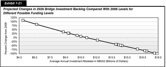
| Annual Percent Change Relative to 2006 | Average Annual Capital Investment (Billions of 2006 Dollars) 1 Total Capital Outlay |
Average Annual Capital Investment (Billions of 2006 Dollars) 1 Spending Modeled in NBIAS |
2026 Bridge Investment Backlog for System Rehabilitation (Billions of 2006 Dollars) 2 Replacement |
2026 Bridge Investment Backlog for System Rehabilitation (Billions of 2006 Dollars) 2 Improvement (Raising, Strengthening, and Widening) |
2026 Bridge Investment Backlog for System Rehabilitation (Billions of 2006 Dollars) 2 Rehabilitation and Repair |
2026 Bridge Investment Backlog for System Rehabilitation (Billions of 2006 Dollars) 2 Total |
Percent Change in Bridge Backlog Compared to 2006 |
|---|---|---|---|---|---|---|---|
| 5.15% | $139.0 | $17.9 | $0.0 | $0.0 | $0.0 | $0.0 | -100.0% |
| 5.03% | $137.1 | $17.6 | $2.0 | $0.0 | $1.4 | $3.5 | -96.5% |
| 4.65% | $131.2 | $16.9 | $8.5 | $0.5 | $6.5 | $15.5 | -84.3% |
| 4.55% | $129.7 | $16.7 | $10.0 | $0.6 | $7.7 | $18.3 | -81.5% |
| 4.17% | $124.2 | $16.0 | $16.8 | $1.3 | $10.4 | $28.5 | -71.2% |
| 3.30% | $112.6 | $14.5 | $33.2 | $2.1 | $14.4 | $49.7 | -49.7% |
| 3.21% | $111.5 | $14.4 | $35.0 | $2.1 | $14.7 | $51.8 | -47.6% |
| 3.07% | $109.7 | $14.1 | $37.8 | $2.2 | $14.9 | $55.0 | -44.4% |
| 2.96% | $108.4 | $14.0 | $39.8 | $2.3 | $15.1 | $57.1 | -42.2% |
| 2.93% | $108.0 | $13.9 | $40.4 | $2.3 | $15.1 | $57.8 | -41.5% |
| 1.67% | $94.0 | $12.1 | $63.9 | $3.0 | $16.5 | $83.4 | -15.6% |
| 0.83% | $85.9 | $11.1 | $78.4 | $3.2 | $17.2 | $98.8 | 0.0% |
| 0.34% | $81.5 | $10.5 | $86.1 | $3.3 | $17.6 | $107.0 | 8.2% |
| 0.00% | $78.7 | $10.1 | $91.3 | $3.4 | $17.8 | $112.6 | 13.9% |
| -0.78% | $72.5 | $9.3 | $104.0 | $3.5 | $18.4 | $125.8 | 27.3% |
| -0.86% | 71.9 | $9.3 | $105.3 | $3.5 | $18.4 | $127.2 | 28.6% |
| -1.37% | $68.3 | $8.8 | $112.5 | $3.6 | $18.7 | $134.8 | 36.4% |
| -4.95% | $48.2 | $6.2 | $156.8 | $3.7 | $20.4 | $180.9 | 83.0% |
| -7.64% | $37.9 | $4.9 | $181.2 | $3.8 | $21.0 | $206.0 | 108.3% |
| 2006 Baseline Values: | $98.9 | ||||||
Exhibit 7-21 also identifies separate components of the overall bridge investment backlog, identifying the portion associated with bridge replacement; bridge improvement, including the raising, strengthening, and widening of existing bridges; and bridge rehabilitation and repair. The reason that most of the backlog is associated with bridge replacement is that these are the investments that NBIAS tends to defer when available funding is constrained as the high capital costs associated with them frequently causes their benefit-cost ratios to be lower than potential improvement, rehabilitation, or repair actions.
NBIAS computes the average benefit-cost ratio for bridge improvements to be somewhere in the range of 3.5 to 10.2 depending on the overall level of investment being implemented, compared to an average benefit-cost ratio of 1.7 to 2.8 for bridge rehabilitation and repair actions, and an average benefit-cost ratio of 1.4 to 2.1 for bridge replacement actions. The marginal benefit-cost ratios associated with these averages are naturally lower, in that marginal ratios pertain to the last, and least cost-beneficial, project funded within a given budget. NBIAS estimates that the lowest benefit-cost ratio for any project implemented in 2026 would be 1.0 if spending grows at an annual rate of 5.15 percent, approximately 1.2 if spending grows at 1.67 percent annually, and approximately 1.5 if spending declines by 0.78 percent per year. It should be noted that the computation of benefit-cost ratios in NBIAS is not as robust as that in HERS, and that the model may not be capturing the full range of benefits associated with certain types of bridge investments, particularly in regards to keeping bridges open and thus avoiding detours.
Impacts of NHS Investments Modeled by NBIAS
Exhibit 7-22 identifies the portion of the total economic bridge investment backlog that is attributable to bridges on the NHS, and how that backlog would be influenced by the amount of combined public and private investment on the NHS for types of capital improvements modeled in NBIAS. The first 19 investment levels described in Exhibit 7-22 correspond to the systemwide spending levels in Exhibit 7-21; the next row has been included to specifically identify the costs associated with maintaining the NHS bridge backlog at its 2006 level of $50.8 billion, while the last row shows the impacts of sustaining investment on the NHS at 2006 levels in constant dollar terms.
| Annual Percent Change Relative to 2006 | Average Annual Capital Investment (Billions of 2006 Dollars) 1 Total Capital Outlay |
Average Annual Capital Investment (Billions of 2006 Dollars) 1 Spending Modeled in NBIAS Total |
Average Annual Capital Investment (Billions of 2006 Dollars) 1 Spending Modeled in NBIAS On NHS |
2026 NHS Bridge Backlog 2 (Billions of 2006 Dollars) | Percent Change in Bridge Backlog Compared to 2006 |
|---|---|---|---|---|---|
| 5.15% | $139.0 | $17.9 | $7.7 | $0.0 | -100.0% |
| 5.03% | $137.1 | $17.6 | $7.6 | $1.3 | -97.4% |
| 4.65% | $131.2 | $16.9 | $7.4 | $5.3 | -89.6% |
| 4.55% | $129.7 | $16.7 | $7.3 | $6.2 | -87.8% |
| 4.17% | $124.2 | $16.0 | $7.1 | $10.1 | -80.1% |
| 3.30% | $112.6 | $14.5 | $6.5 | $18.4 | -63.8% |
| 3.21% | $111.5 | $14.4 | $6.5 | $19.4 | -61.8% |
| 3.07% | $109.7 | $14.1 | $6.4 | $20.9 | -58.9% |
| 2.96% | $108.4 | $14.0 | $6.3 | $22.4 | -55.9% |
| 2.93% | $108.0 | $13.9 | $6.3 | $22.6 | -55.5% |
| 1.67% | $94.0 | $12.1 | $5.6 | $34.5 | -32.1% |
| 0.83% | $85.9 | $11.1 | $5.1 | $42.4 | -16.5% |
| 0.34% | $81.5 | $10.5 | $4.9 | $46.0 | -9.4% |
| 0.00% | $78.7 | $10.1 | $4.8 | $48.2 | -5.1% |
| -0.78% | $72.5 | $9.3 | $4.5 | $54.1 | 6.5% |
| -0.86% | $71.9 | $9.3 | $4.5 | $54.6 | 7.5% |
| -1.37% | $68.3 | $8.8 | $4.3 | $57.8 | 13.8% |
| -4.95% | $48.2 | $6.2 | $3.2 | $78.4 | 54.3% |
| -7.64% | $37.9 | $4.9 | $2.5 | $91.1 | 79.3% |
| Cost to Maintain:3 | $4.7 | $50.8 | 0.0% | ||
| 2006 Spending:4 | $4.3 | $57.3 | 12.8% | ||
| 2006 Baseline Values: | $4.3 | $50.8 | |||
Exhibit 7-22 shows that if combined public and private highway capital investment on types of improvements modeled in NBIAS were sustained in constant dollar terms at their current level of $10.1 billion, the model would recommend that $4.8 billion be directed to the NHS; this is above the $4.3 billion identified in Exhibit 7-1 as having been spent on the NHS for NBIAS-modeled improvement types in 2006. It is projected that this level of investment would result in a decrease in the economic backlog for NHS bridges of approximately 5.1 percent. NBIAS predicts that the economic backlog for NHS bridges could be maintained at base year levels if average annual investment on the NHS for the types of improvements modeled in NBIAS were to rise to $4.7 billion in constant 2006 dollars, while the economic backlog could potentially be eliminated by an investment averaging approximately $7.7 billion annually in constant 2006 dollars.
Impacts of Interstate Investments Modeled by NBIAS
Exhibit 7-23 describes how the economic backlog for Interstate bridges could be influenced by the amount of combined public and private investment on the Interstate System for the types of capital improvements modeled in NBIAS. The first 19 investment levels described in Exhibit 7-23 correspond to the systemwide spending levels in Exhibit 7-21. The next row has been included to specifically identify the costs associated with maintaining the Interstate bridge backlog at its 2006 level of $33.4 billion, while the last row shows the impacts of sustaining investment on Interstate bridges at 2006 levels in constant dollar terms.
| Annual Percent Change Relative to 2006 | Average Annual Capital Investment (Billions of 2006 Dollars) 1 Total Capital Outlay |
Average Annual Capital Investment (Billions of 2006 Dollars) 1 Spending Modeled in NBIAS Total |
Average Annual Capital Investment (Billions of 2006 Dollars) 1 Spending Modeled in NBIAS On Interstate |
2026 Interstate Bridge Backlog 2 (Billions of 2006 Dollars) | Percent Change in Bridge Backlog Compared to 2006 |
|---|---|---|---|---|---|
| 5.15% | $139.0 | $17.9 | $4.7 | $0.0 | -100.0% |
| 5.03% | $137.1 | $17.6 | $4.6 | $0.7 | -97.9% |
| 4.65% | $131.2 | $16.9 | $4.5 | $2.8 | -91.6% |
| 4.55% | $129.7 | $16.7 | $4.5 | $3.2 | -90.4% |
| 4.17% | $124.2 | $16.0 | $4.3 | $5.3 | -84.1% |
| 3.30% | $112.6 | $14.5 | $4.0 | $10.9 | -67.4% |
| 3.21% | $111.5 | $14.4 | $4.0 | $11.5 | -65.6% |
| 3.07% | $109.7 | $14.1 | $3.9 | $12.7 | -62.0% |
| 2.96% | $108.4 | $14.0 | $3.7 | $12.9 | -61.4% |
| 2.93% | $108.0 | $13.9 | $3.8 | $14.1 | -57.8% |
| 1.67% | $94.0 | $12.1 | $3.4 | $21.9 | -34.4% |
| 0.83% | $85.9 | $11.1 | $3.1 | $26.9 | -19.5% |
| 0.34% | $81.5 | $10.5 | $3.0 | $29.3 | -12.3% |
| 0.00% | $78.7 | $10.1 | $2.9 | $30.8 | -7.8% |
| -0.78% | $72.5 | $9.3 | $2.7 | $34.7 | 3.9% |
| -0.86% | $71.9 | $9.3 | $2.7 | $35.1 | 5.1% |
| -1.37% | $68.3 | $8.8 | $2.6 | $37.0 | 10.8% |
| -4.95% | $48.2 | $6.2 | $1.8 | $48.1 | 44.0% |
| -7.64% | $37.9 | $4.9 | $1.5 | $58.8 | 76.0% |
| Cost to Maintain:3 | $2.8 | $33.4 | 0.0% | ||
| 2006 Spending:4 | $2.5 | $39.1 | 17.1% | ||
| 2006 Baseline Values: | $2.5 | $33.4 | |||
Exhibit 7-23 shows that if combined public and private highway capital investment on the types of improvements modeled in NBIAS were sustained in constant dollar terms at their current level of $10.1 billion, the model would recommend that $2.9 billion be directed to the Interstate; this is above the $2.5 billion identified in Exhibit 7-1 as having been spent on the Interstate for NBIAS-modeled improvement types in 2006. It is projected that this level of investment would result in a decrease in the economic backlog for Interstate NHS bridges of approximately 7.8 percent. NBIAS predicts that the economic backlog for Interstate bridges could be maintained at base year levels if average annual investment on the Interstate for the types of improvements modeled in NBIAS were to rise to $2.8 billion in constant 2006 dollars, while the economic backlog could potentially be eliminated by an investment averaging approximately $4.7 billion annually in constant 2006 dollars.
Potential Transit Capital Investment Impacts
This section of the 2008 C&P Report examines how different types and levels of annual capital investments would affect measures of transit system condition and performance by 2026. The analysis presented in this chapter begins with an overview of the types of capital spending projected by the Transit Economic Requirements Model (TERM). The chapter then moves into an examination of how different annual spending levels impact transit system conditions and performance on a national basis before continuing on with an analysis of how various levels of annual expenditures affect various urbanized areas (UZAs) characterized by differing transit environments.
Types of Capital Spending Projected by TERM
As stated elsewhere in this report, the Federal Transit Administration (FTA) uses TERM, an analysis tool based on engineering and economic concepts, to forecast estimates of total capital investment needs for the U.S. transit industry over a 20-year period. The model uses data from a variety of sources, including State and local transit agencies, the National Transit Database (NTD), and regional Metropolitan Planning Organizations (MPOs) to generate its estimates.
TERM identifies potential investments using asset decay curves relating transit asset condition to age, and in some cases additionally to maintenance and use. TERM also identifies investment levels necessary to achieve stated performance goals based on measures such as vehicle occupancy rates and passenger travel times. The model subsequently uses benefit-cost analysis techniques to limit the actual level of investment forecast to a subgroup of the total investments identified. Investments with benefit-cost ratios of 1.0 or greater are added to the forecast while those with ratios less than one are excluded.
Using the data and techniques described above, TERM develops a forecast that consists of a collection of various investment types that U.S. transit agencies typically undertake to maintain and in some cases improve operations. Specifically, the model forecasts investments intended to: (1) rehabilitate and replace existing assets that are in a state of disrepair or past their useful life; (2) expand the existing transit asset base as required to maintain current performance levels (measured by average riders per vehicle) given projected growth in ridership; and (3) improve performance both for those agency-modes currently experiencing system overcrowding and for those metropolitan areas with transit operating speeds that are well below the national average. All capital investments forecast by TERM must successfully pass the model's benefit-cost analysis before being added to the tally of the Nation's investment needs.Rehabilitation and Replacement Investments
For the analysis presented in this chapter, TERM estimates the total investment required for ongoing rehabilitation and replacement of the Nation's existing transit assets over a 20-year period. In estimating these types of investments, the model predicts reinvestment in a number of areas, including existing fleet vehicles, maintenance facilities, stations, guideway and trackwork, and train control and traction power systems. The model starts with a detailed inventory of all U.S. transit assets as its foundation and then applies a set of asset-specific decay curves to determine when discrete transit assets in the inventory will require rehabilitation or replacement over the 20-year forecast period under consideration. TERM then records these expenditures, minus any investments that did not pass the model's benefit-cost test, in a tally of national transit capital needs.
| What types of capital spending are not modeled by TERM? | |
|
TERM does not project all types of capital spending undertaken by U.S. transit agencies. Specifically, the model does not forecast capital expenditures:
It is important to note that, while TERM does not forecast the types of expenditures described above, some of these investment types (but not all) are included in the actual capital expenditures accounted for in this report, which are taken from information submitted to the NTD by local transit agencies.
|
|
The specific rehabilitation and replacement needs estimated by TERM include:
- Elimination of any investment backlog ("deferred investment")
- Routine replacement of assets reaching the end of their useful life
- Mid-life asset rehabilitations
- Annual capital expenditures required to maintain a state of good repair
At the end of a model run, TERM is capable of reporting these investments by mode, asset type, local agency, UZA, State, or FTA region.
Expansion Investments
In addition to the ongoing rehabilitation and replacement of existing assets, agencies also devote a portion of their capital budgets to the procurement or construction of new or expansion assets, including additional vehicles, stations, and new rail guideway and facilities beyond those already in service. Investments in expansion assets can be thought of as serving two distinct purposes. First, the demand for transit services typically increases over time in line with population growth, employment and other factors. To maintain current levels of performance in the face of expanding demand, transit operators must similarly expand the capacity of their services (e.g., an agency may add revenue service vehicles to an existing bus fleet). Failure to accommodate this demand would result in increased vehicle crowding, increased dwell times and decreased operating speeds for existing services. Second, transit operators also invest in expansion projects with the aim of improving current service performance. Such improvements include capital expansion projects (e.g., a new light rail segment) to reduce vehicle crowding or increase average operating speeds. (It is important to note that performance-improving investments are distinct from investments intended to improve the functional aspects of existing assets, which are not estimated by TERM, as described in Q&A box above.)
TERM is designed to address both of these issues. The model, however, forecasts investments to maintain current service standards separately from investments to improve service standards by employing two distinct modules, allowing the FTA to report the investment forecasts to address each need independently.
Expansion Investments: Maintain Performance
For measures undertaken to maintain existing service levels, the model estimates the amount of investment in new expansion assets that would be required to maintain the quality of existing transit services given projected growth in travel demand. TERM first estimates the rate of growth in transit vehicle fleets required to maintain current vehicle occupancy levels given the anticipated growth rate in transit passenger miles by UZA. The model also forecasts investments in the expansion of other assets needed to support projected fleet growth, including bus maintenance facilities and, in the case of rail systems, additional investment in guideway, trackwork, stations, maintenance facilities, train control, and traction power systems. Asset expansion investment needs are assessed for all agencies reporting to the NTD on a mode-by-mode basis. Note that TERM does not invest in asset expansion for those agency-modes whose current ridership is well below the national average (specifically, where the performance metric of riders per peak vehicle is more than one standard deviation below the national average).
Expansion Investments: Improve Performance
In addition to forecasting investments intended to preserve existing service performance levels, TERM is designed to estimate the level of investment required to improve service performance. Specifically, TERM forecasts two types of performance enhancing investments intended to meet the following objectives:
- Increase average operating speeds for UZAs that are well below the national mean
- Reduce vehicle occupancy for agencies with the highest ratios of passenger trips per peak vehicle
In forecasting speed improvement investments, TERM first identifies each UZA with an average transit operating speed well below the national average. The model then estimates the minimum required investment in a high-speed transit mode (i.e., heavy rail, light rail, or bus rapid transit) required to reach a minimum performance standard, defined as the national average operating speed less one standard deviation. The determination of which high-speed mode to invest in is based on which high-speed modes already exist in that particular UZA; if there is currently no high-speed mode in the UZA, TERM selects a preferred mode of investment based on UZA size. UZAs with populations of less than 1 million are designated to receive bus rapid transit systems, while larger UZAs are designated as recipients of light rail systems. Finally, as with performance maintenance investment forecasts, TERM does not undertake speed-improving investments in UZAs with low levels of reported ridership.
As part of predicting investments to improve performance, TERM also identifies local agency-modes with high vehicle occupancy rates (i.e., high ridership per peak vehicle relative to the national average for that mode). The model then designates investments that provide additional fleet capacity as needed to reduce peak vehicle crowding on these agency-modes to an acceptable level of service, defined as the national average of riders per peak vehicle plus one standard deviation for that mode. If the increase in fleet size is sufficiently large, TERM will also project investments in additional expansion assets such as maintenance facilities and, for rail systems, additional route miles, including guideway, trackwork, stations, train control, and traction power systems.
TERM's Benefit-Cost Tests
As stated above, all investments estimated by TERM must successfully pass the model's benefit-cost analysis in order to be added to the tally of the Nation's investment needs. If an investment fails the benefit-cost test (by receiving a benefit-cost ratio of less than one), it is rejected and its costs are not added to the overall investment tally. If the investment passes the benefit-cost test, the investment needs tally is updated to include the investment costs. All of TERM's benefit-cost tests evaluate each proposed investment over a 20-year time period.
Exhibit 7-24 presents the amount of actual capital spending on transit systems in 2006 that corresponds to the investment types modeled in TERM. Of the $12.8 billion spent by U.S. transit agencies on capital projects in 2006, $9.3 billion or 72.7 percent was devoted to rehabilitating and replacing existing assets. The remaining $3.5 billion or 27.3 percent was spent on performance maintenance and improvement investments.
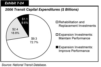
Impact of Systemwide Investments Modeled by TERM
The specific annual capital spending levels shown in the exhibits in this section typically relate to a particular point of interest. For example, Exhibit 7-25 presents the expected impact of different levels of average annual capital investment in rehabilitation and replacement investments on average transit assets conditions by the year 2026. Conversely, Exhibit 7-26, Exhibit 7-27 and Exhibit 7-28 consider the level of investment in expansion assets as required to support differing rates of ridership growth and differing levels of transit performance. The FTA used TERM to produce all analyses.
Impact of Rehabilitation and Replacement Investments on Transit Conditions
Exhibit 7-25 provides a summary of the impact of differing levels of annual rehabilitation and replacement investments on the future condition of U.S. transit assets. The graph shows the relationship between varying annual expenditures on rehabilitation and replacement activities and the impact of those expenditures on national average transit conditions, with transit conditions improving as annual capital spending increases. Note that the investment levels presented only include those investments that pass TERM's internal benefit-cost test. It is also important to note that the needs estimates shown in Exhibit 7-25 include investment needs modeled by TERM as well as investment needs not modeled by TERM, such as capital spending intended to improve safety. For this reason, the capital needs estimates shown here are not directly comparable to the needs estimates shown in Chapter 8.
| Average Annual Percent Change vs. 2006 | Average Annual Investment ($2006 B) Total Capital Outlay1 |
Average Transit Conditions in 20262 Asset Categories Guideway |
Average Transit Conditions in 20262 Asset Categories Facilities |
Average Transit Conditions in 20262 Asset Categories Systems |
Average Transit Conditions in 20262 Asset Categories Stations |
Average Transit Conditions in 20262 Asset Categories Vehicles |
Average Transit Conditions in 20262 All Transit Assets |
Funding Level Description |
|---|---|---|---|---|---|---|---|---|
| 3.1% | $13.0 | 4.33 | 3.84 | 3.88 | 3.16 | 3.52 | 3.85 | Replace at Condition 3.00 |
| 2.1% | $11.6 | 4.22 | 3.50 | 3.74 | 3.01 | 3.47 | 3.70 | Improve Conditions |
| 1.7% | $11.1 | 4.07 | 3.48 | 3.71 | 3.01 | 3.39 | 3.64 | Maintain Conditions |
| 0.8% | $10.1 | 3.98 | 3.00 | 3.66 | 3.04 | 3.34 | 3.51 | |
| 0.0% | $9.3 | 3.97 | 2.91 | 3.65 | 3.00 | 3.26 | 3.46 | 2006 Capital Expenditures |
| -1.0% | $8.4 | 3.91 | 2.89 | 3.58 | 2.99 | 3.08 | 3.39 | |
| -2.5% | $7.2 | 3.85 | 2.85 | 3.38 | 2.97 | 2.98 | 3.31 | |
| -10.6% | $3.5 | 3.67 | 2.82 | 2.99 | 2.74 | 2.91 | 3.16 |
The table in Exhibit 7-25 presents the same investment and average condition information as the chart above it. This table also presents the average annual percentage increase in constant dollar funding from today's level to achieve each projected condition level and the projected average condition values for transit assets by asset type (in addition to the average value across all asset types).
The vertical line on the graph in Exhibit 7-25 signifies that U.S. transit agencies spent $9.3 billion in 2006 to rehabilitate and replace antiquated and/or worn equipment. If sustained into the future on an annual basis, TERM estimates that this level of investment would correspond with a national average condition rating of 3.32 for all assets in 2026, a condition below the current average condition rating of 3.55. The average condition of the different asset categories in 2026 under this funding scenario would range between marginal and good as defined in Chapter 3.
To maintain the existing average condition of U.S. transit assets, agencies would need to increase annual capital spending in constant dollars on rehabilitation and replacement activities by a combined 1.2 percent each year through 2026. This would be equivalent to increasing the current annual level of spending on rehabilitation and replacement from $9.3 billion to an annual average level of $11.4 billion from today through 2026. (Note that the $11.4 billion estimate to maintain conditions includes $10.5 billion in capital spending modeled by TERM plus an additional $0.89 billion for capital spending not estimated by the model—including investments in betterments, safety, and other improvements. Moreover, TERM's $10.5 billion needs estimate to maintain current conditions is not directly comparable to the $10.7 billion cited in Chapter 8 because the latter also includes the investment needs of special service operators.) TERM predicts that this level of capital investment would ensure that the average condition rating of existing transit assets remain at the current level of 3.55 in 2026, depicted by the horizontal line in the graph.
| What is the significance of the Replace at Condition 2.5 threshold? | |
|
The Replace at Condition 2.5 threshold is significant as it relates to the Rail Modernization study, released by FTA in April 2009. A state of good repair, for the purposes of the study, was defined using TERM's numerically based condition rating scale of 1 to 5 (poor to excellent) for evaluating transit asset conditions. An asset or a transit system is considered to be in a state of good repair if the asset or system has an estimated condition value of 2.5 or higher (the mid-point between adequate and marginal). The level of investment required to attain and maintain a state of good repair is therefore that amount required to rehabilitate and replace all assets with estimated condition ratings that are less than this minimum condition value.
|
|
To improve the average condition rating of transit assets to 3.67, TERM forecasts that agencies would need to accelerate annual spending even more, from $9.3 billion to an average of $13.0 billion through 2026. This would be equivalent to increasing current levels of annual capital expenditures by an average of 2.3 percent each year.
Finally, if transit agencies adopted more aggressive policies for replacing capital assets once their condition ratings deteriorated to 3.0, capital expenditures would need to increase to $14.4 billion per year through 2026 (which is equivalent to a 3.2 percent average annual increase). This level of annual spending on rehabilitation and replacement activities, according to estimates made by TERM, would increase the average condition rating of all assets from a current level of 3.55 to an average of 3.76 by the year 2026.
Impact of All Expansion Investments on Transit Ridership
While capital spending on rehabilitation and replacement initiatives primarily benefits the physical condition of transit assets, expansion investments are typically undertaken to accommodate projected growth in ridership and/or to improve service performance (the result of which encourages additional ridership).
Exhibit 7-26 shows the relationship between annual capital spending on expansion investments and the additional number of annual passenger boardings that transit systems would be able to support by 2026. It is important to note that this exhibit presents the combined impact of two types of expansion investments. This includes expansions to maintain current system performance given projected growth in transit ridership (such that the current annual number of riders per peak vehicle is maintained) and investments to improve performance for those transit systems with high vehicle occupancies or low average operating speeds (by further expanding existing capacity or introducing new rail services). Each of these two investment types are considered in greater detail in subsequent sections. The exhibit illustrates the implied average annual growth in new riders directly supported by these investments. The upward sloping curve of the graph indicates that higher levels of investment are required to support greater numbers of riders, ensuring that current vehicle occupancy rates are maintained through 2026.
| Average Annual Percent Change vs. 2006 | Average Annual Investment ($2006 B) | Total New Boardings and Vehicle Capacity Utilization by 2026 New Riders Supported (Billions of Annual Boardings) |
Total New Boardings and Vehicle Capacity Utilization by 2026 Average Annual Growth in Boardings* |
Funding Level Description |
|---|---|---|---|---|
| 9.5% | $10.2 | 4.12 | 1.8% | Improve Performance |
| 1.5% | $4.1 | 3.21 | 1.5% | Projected Increase in Boardings by 2026 |
| 1.0% | $3.9 | 3.11 | 1.4% | |
| 0.0% | $3.5 | 2.91 | 1.3% | 2006 Capital Expenditures (all expansion) |
| -2.5% | $2.7 | 2.67 | 1.2% | |
| -5.0% | $2.1 | 2.48 | 1.2% | |
| -10.0% | $1.4 | 2.15 | 1.0% | |
| -20.0% | $0.7 | 1.55 | 0.8% | |
| -50.0% | $0.2 | 0.53 | 0.3% |
As shown by the vertical line on the graph in Exhibit 7-26, U.S. transit agencies spent $3.5 billion on expansion investments in 2006. This level of annual funding for expansion projects, if preserved over a 20-year period, could allow U.S. transit service providers to support 2.91 billion new passenger boardings by 2026. As demonstrated in the exhibit, keeping expenditures at 2006 levels could support 1.3 percent average annual growth in new passenger boardings.
The Nation's MPOs expect passenger boardings to increase at an annual rate of 1.5 percent. To accommodate this level of anticipated growth, transit operators would need to increase annual capital spending on expansion investments to $4.1 billion annually from their current annual level of about $3.5 billion, an amount equivalent to a 1.5 percent average annual increase in expansion expenditures through 2026. TERM forecasts that this level of annual funding could support 3.21 billion additional annual passenger boardings by 2026 (represented by the horizontal line on the graph in Exhibit 7-26), while maintaining vehicle occupancy rates at current levels. It is important to emphasize here that the preceding scenario represents the level of capital investment required to maintain current service performance levels, given the projected 1.5 percent average annual growth in passenger boardings. Some natural growth in ridership will occur regardless of whether the transit industry invests in advance of the projected increase. However, in the absence of investment to accommodate that ridership increase, it should be anticipated that average vehicle occupancies would increase and result in a decline in service performance from today's levels.
Conversely, if transit operators wish to support the number of new boardings anticipated in 2026 and improve the performance of their systems, they would need to allocate an even higher level of capital funds for expansion investments. For example, Exhibit 7-26 presents the annual capital spending on expansion projects required both to maintain current transit performance levels on all systems and to improve performance on systems with high vehicle occupancies and/or with low operating speeds (this specific scenario is described further in Chapter 8). To improve performance, the level of annual capital funds expended on expansion investments would need to increase to $10.2 billion, which is $6.7 billion more than the amount spent in 2006.
The analysis in Exhibit 7-26 has considered expansion investments designed to both maintain current performance (i.e., vehicle occupancies) and improve performance. The next two sections consider the expected performance impacts of these two types of expenditures under differing levels of investment.
Impact of Performance Maintenance Investments
Transit agencies that serve markets with increasing demand in ridership would need to make investments to expand service capacity in order to maintain performance at current service levels. In the absence of investing in such expansion projects, ridership growth would result in an increased number of riders per vehicle and furthermore may also lead to decreasing operating speeds. The decrease in operating speeds would be a direct result of larger volumes of riders who would otherwise board and alight from the same, fixed number of revenue vehicles. To prevent this from occurring, agencies experiencing and anticipating new growth would need to invest continually in additional capacity to accommodate ridership while maintaining current performance.
Exhibit 7-27 shows the relationship between investments made to maintain existing performance and new annual passenger boardings supported by those investments by the year 2026. The graph clearly indicates that increased levels of annual capital spending would support more new passenger boardings by 2026. The exhibit also depicts the capacity utilization (defined as passengers per vehicle) for commuter rail, heavy rail, light rail, and motor bus vehicles under the various funding scenarios assuming that the 1.5 percent annual increase in ridership as projected by the Nation's MPOs is fully realized. Under this assumption, investment at levels lower than required to maintain performance will necessarily result in increased capacity utilization (i.e., crowding) and hence decreased system performance.
| Average Annual Investment ($2006 B) | Total New Boardings and Vehicle Capacity Utilization by 2026 New Riders Supported (Billions of Annual Boardings) |
Total New Boardings and Vehicle Capacity Utilization by 2026 Average Annual Growth in Boardings* |
Total New Boardings and Vehicle Capacity Utilization by 2026 Passengers Per Vehicle (Assuming MPO Growth Rate Projections) Commuter Rail |
Total New Boardings and Vehicle Capacity Utilization by 2026 Passengers Per Vehicle (Assuming MPO Growth Rate Projections) Heavy Rail |
Total New Boardings and Vehicle Capacity Utilization by 2026 Passengers Per Vehicle (Assuming MPO Growth Rate Projections) Light Rail |
Total New Boardings and Vehicle Capacity Utilization by 2026 Passengers Per Vehicle (Assuming MPO Growth Rate Projections) Motor Bus |
Funding Level Description |
|---|---|---|---|---|---|---|---|
| $5.8 | 5.51 | 2.3% | 32.30 | 20.24 | 22.68 | 8.85 | Growth 50% higher than forecast |
| $4.3 | 3.35 | 1.5% | 36.85 | 24.29 | 30.34 | 10.97 | MPO projected increase in boardings |
| $4.0 | 3.16 | 1.4% | 36.85 | 25.33 | 30.34 | 10.98 | |
| $2.8 | 2.71 | 1.3% | 37.02 | 29.00 | 30.34 | 11.01 | |
| $1.5 | 2.53 | 1.2% | 39.49 | 26.36 | 30.34 | 11.21 | 2006 Capital Expenditures (maintain performance investments) |
| $1.5 | 2.28 | 1.1% | 44.37 | 30.71 | 33.96 | 11.41 | |
| $1.0 | 1.88 | 0.9% | 46.82 | 30.71 | 41.54 | 12.18 | |
| $0.5 | 1.11 | 0.5% | 46.82 | 30.71 | 53.99 | 13.48 | |
| $0.3 | 0.64 | 0.3% | 46.82 | 30.71 | 53.99 | 14.92 |
In 2006, as depicted by the vertical line on the graph in Exhibit 7-27, transit agencies spent an estimated $2.4 billion to expand the capacity of existing transit infrastructure. If continued, TERM predicts that this level of annual capital spending would allow U.S. transit operators to accommodate 2.53 billion additional passenger boardings by 2026, causing capacity utilization rates for most modes of transit to increase. For example, the average number of riders per vehicle is projected to increase from 10.97 to 11.21 passengers for motor bus, from 36.85 to 39.49 for commuter rail, and from 24.29 to 29.36 for heavy rail; in contrast, light rail's average number of riders is projected to remain the same at 30.34.
Passenger boardings, as projected by the Nation's MPOs, are expected to grow at an average rate of 1.5 percent per year. This means that U.S. transit operators should expect demand for transit services to increase by 3.35 billion passenger boardings. This increased level is depicted by the horizontal line in the graph in Exhibit 7-27. To maintain performance standards in the wake of the anticipated increase in demand, it is projected that transit service providers would need to increase annual capital spending on projects that maintain performance to an estimated average annual level of $4.3 billion per year, up $1.9 billion per year from the current annual spending level of $2.4 billion. TERM estimates that this level of annual capital spending would ensure that current vehicle capacity utilization rates for all modes are maintained through 2026.
If total ridership were to increase 50 percent more than currently projected (i.e., if ridership growth reaches 2.3 percent per year versus the forecast of 1.5 percent per year growth), average annual capital expenditures on performance maintaining investments would need to increase to $5.8 billion through 2026. This could permit transit service providers to accommodate 5.51 billion additional annual passenger boardings by 2026 while maintaining current vehicle capacity utilization. (It is important to note that the passengers per vehicle numbers in Exhibit 7-27 represent expected capacity utilization if the transit ridership expands at the rate projected by the nation's MPOs. For example, on the top line of Exhibit 7-27, the passenger per vehicle numbers represent expected capacity utilization if the transit industry expands to accommodate a 2.3 percent annual ridership increase; but, this would occur only if a 1.5 percent annual growth materializes. This would imply a drop in capacity utilization.)
Impact of Performance-Improving Investments
In addition to making investments intended to maintain existing performance standards, U.S. transit agencies also invest in additional assets, such as vehicles and supporting infrastructure, to improve the performance of their operations. As described above, TERM considers two types of performance-improving investments. The first expands the revenue vehicle fleets and related supporting infrastructure of existing transit operations that are currently overcrowded as defined by TERM. The second invests in new guideway systems (e.g., heavy rail, light rail or bus rapid transit, depending on the size of the urbanized area and the presence of any preexisting rail modes) as needed to improve the overall average speed of transit in the specific urbanized area where the average transit operating speed is well below the national average.
Exhibit 7-28 shows the relationship between annual performance improvement expenditures and new passenger boardings generated by those investments by 2026 and reflects TERM's preferential investment in those projects with the highest benefit-cost ratios (which tend to translate into higher ridership benefits per investment dollar). In other words, TERM invests first in those projects with the highest ridership benefits (on the left hand side of the graph) followed by investment in less beneficial projects as the overall level of expenditure increases (on the right hand side).
| Average Annual Investment ($2006 B) | Total New Ridership by 2026 New Annual Boardings by 2026 (Billions) |
Total New Ridership by 2026 Average Annual Growth in New Boardings1 |
Total New Ridership by 2026 Capacity Utilization2 Heavy Rail |
Total New Ridership by 2026 Capacity Utilization2 Light Rail |
Total New Ridership by 2026 Capacity Utilization2 Motor Bus |
Average Transit Operating Speed (MPH) | Funding Level Description |
|---|---|---|---|---|---|---|---|
| $6.1 | 1.08 | 0.54% | 26.02 | 31.66 | na | 13.60 | Improve performance target |
| $2.2 | 0.98 | 0.49% | 27.97 | 32.46 | na | 13.12 | |
| $1.7 | 0.89 | 0.44% | na | 32.49 | na | 13.09 | |
| $1.4 | 0.85 | 0.43% | na | 32.49 | na | 13.08 | |
| $1.2 | 0.84 | 0.42% | na | 32.49 | na | 13.06 | |
| $1.1 | 0.81 | 0.41% | na | 32.49 | na | na | 2006 Capital Expenditures (improve performance investments) |
| $1.0 | 0.79 | 0.40% | na | 33.48 | 11.00 | na | |
| $0.8 | 0.76 | 0.38% | na | na | 11.06 | na | |
| $0.6 | 0.62 | 0.32% | na | na | 11.25 | na | |
| $0.3 | 0.35 | 0.18% | na | na | 12.02 | na |
Exhibit 7-28 also displays capacity utilization for heavy rail, light rail, and motor bus, as well as the average transit operating speed for all modes. Note that these utilization and average operating speed values are only presented for those UZAs, and at those investment levels, where TERM has identified a performance-improving investment (hence an "na" value indicates no new investment at that level of expenditures). The pattern of investments in this table suggests TERM tends to assess the highest benefits per dollar invested for bus and the lowest for heavy rail. It also suggests that investments in capacity improvements for existing transit modes tend to generate higher benefits than those that increase a UZA's overall operating speed.
The vertical line on the left in Exhibit 7-28 indicates that transit agencies spent an estimated $1.1 billion on performance enhancing investments in 2006, a level of spending that would support 0.81 billion additional annual boardings by 2026.
The second vertical line on the graph in Exhibit 7-28 represents the level of investment in constant dollars required to improve the performance of transit operators that tend to experience significant crowding and UZAs with low average operating speeds for transit (the specifics of this "improve performance" scenario are discussed further in Chapter 8). To realize these improvements, transit agencies would need to increase annual expenditures to an estimated level of $6.1 billion. This level of annual spending could support 1.08 billion additional annual passenger boardings by 2026 and would allow the average transit operating speed to increase to 13.6 miles per hour. By increasing capital expenditures to $6.1 billion per year, transit agencies would decrease capacity utilization rates for systems exhibiting the highest utilization rates.
Impact of Investments Modeled by TERM
The remainder of this chapter focuses on how different levels of annual capital investment in the U.S. transit infrastructure affect urbanized areas with dissimilar transit investment needs. Specifically, this section explores the impact of capital expenditures by transit agencies grouped into one of three distinct UZA groupings: (1) large metropolitan areas with heavy rail transit systems; (2) large metropolitan areas without heavy rail transit systems; and (3) smaller metropolitan and rural areas.
The figures below reveal that there are significant differences between the supply of and demand for public transportation services within the different types of urbanized areas. As shown in Exhibit 7-29, one of the fundamental differences lies in the fact that, as a group, smaller metropolitan and rural areas are served by a plethora of small- and medium-sized transit agencies. In 2006, there were 1,765 transit agencies operating in cities with populations of less than 1 million. This contrasts sharply with the other two UZA segments: larger cities with heavy rail systems were patronized by 136 agencies in 2006, while cities without heavy rail operators were only served by 97 agencies.
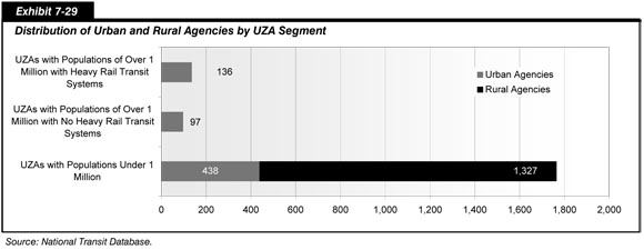
There are also wide discrepancies in the demand for public transportation services in the three different UZA segments. As shown in Exhibit 7-30, total passenger miles varied widely with transit riders in large municipalities, with heavy rail systems consuming 38.3 billion passenger miles in 2006. Passenger miles consumed in these cities in 2006 were more than the total passenger miles recorded for the other two UZA segments combined.
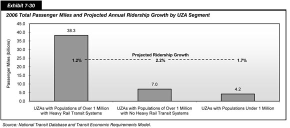
It is interesting to note, however, that the largest cities with heavy rail transit operators are expected to experience the least amount of growth in ridership in the near future. Ridership in large cities without heavy rail transit systems is anticipated to grow at an annual average rate of 2.2 percent, while ridership in smaller cities and rural areas is forecast to increase at a yearly average rate of 1.7 percent.
Transit service providers in these different UZA segments also have unique investments needs, as shown in Exhibit 7-31. Because they tend to operate older, more heavily utilized transportation networks, transit operators in large metropolitan areas with heavy rail transit systems, on average, spend a higher proportion of their capital budgets rehabilitating and replacing existing assets. This is illustrated in Exhibit 7-31, which shows that agencies in these UZAs in 2006 devoted a total of $6.5 billion, or 96.5 percent of their capital spending, to rehabilitation and replacement activities.
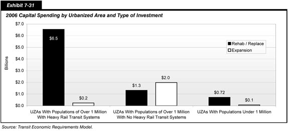
On the other hand, large metropolitan areas lacking heavy rail transit services typically exhibit higher rates of transit ridership growth, creating a need for agencies in these areas to invest in expansion projects. Consequently, when compared to agencies in the first UZA segment, these agencies are likely to devote more capital spending to expansion investments, as shown in Exhibit 7-31. In fact, these operators allocated their capital spending almost equally between rehabilitation/replacement and expansion investments in 2006.
Finally, transit operators in small metropolitan areas have investment needs similar to agencies in cities with heavy rail transit systems because smaller UZAs are not experiencing high absolute levels of transit ridership growth. As shown in Exhibit 7-31, agencies operating in cities with populations of less than 1 million focused a majority of capital spending in 2006 on rehabilitation and replacement investments. Transit service providers in large metropolitan areas with heavy rail transit systems similarly focused the majority of their capital investments on rehabilitating and replacing worn or antiquated assets.
Given the differences between the different UZA segments outlined above, it is instructive to explore the variance in investment needs for the separate groupings. The following analyses explore the effect of both expansion investments and rehabilitation and replacement investments under all three UZA segments.
Urbanized Areas With Populations of More Than 1 Million With Heavy Rail Transit Systems
Large metropolitan areas with heavy rail transit systems represent the most significant share of the Nation's existing investment in transit assets, tend to have high levels of investment in older assets, and have the highest levels of transit use. Most of these cities have mature transit systems and relatively low rates of ridership growth. Key examples of UZAs in this group include New York (including northern New Jersey and western areas of Connecticut), Boston, Philadelphia, Chicago and Washington, D.C. Given these characteristics, these urban areas tend to have the largest rehabilitation and replacement investments needs but lower levels of expansion investments (at least on a percentage growth basis). The following sections of this chapter focus on how rehabilitation and replacement investments, as well as capital spending devoted to expansion projects, affect transit systems in large metropolitan areas with heavy rail transit systems.
Rehabilitation and Replacement Investments
Exhibit 7-32 shows the forecasted impact of rehabilitation and replacement investments on the future condition of transit assets owned by agencies located in large metropolitan areas with heavy rail transit systems. (For this analysis, large metropolitan areas are defined as cities with populations of more than 1 million.)
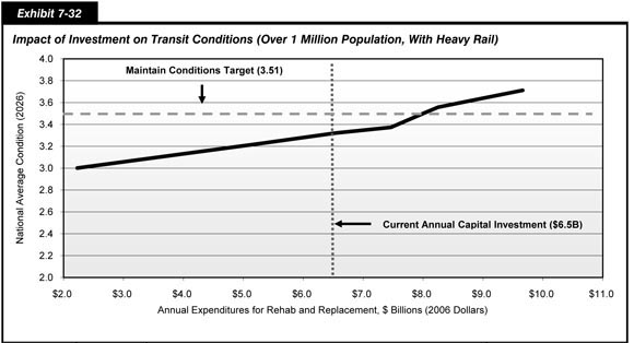
| Average Annual Percent Change vs. 2006 | Average Annual Investment ($2006 B)1 | Average Transit Conditions in 20262 Asset Categories Guideway |
Average Transit Conditions in 20262 Asset Categories Facilities |
Average Transit Conditions in 20262 Asset Categories Systems |
Average Transit Conditions in 20262 Asset Categories Stations |
Average Transit Conditions in 20262 Asset Categories Vehicles |
All Transit Assets | Funding Level Description |
|---|---|---|---|---|---|---|---|---|
| 3.6% | $9.7 | 3.87 | 3.78 | 3.78 | 3.21 | 3.63 | 3.71 | Replace at Condition 3.00 |
| 2.8% | $8.9 | 3.85 | 3.40 | 3.65 | 3.15 | 3.58 | 3.63 | Improve Conditions |
| 2.2% | $8.2 | 3.83 | 3.14 | 3.57 | 3.15 | 3.45 | 3.56 | Maintain Conditions |
| 1.9% | $8.0 | 3.69 | 3.33 | 3.51 | 3.15 | 3.45 | 3.51 | |
| 1.2% | $7.5 | 3.55 | 3.07 | 3.45 | 3.12 | 3.20 | 3.37 | 2006 Capital Expenditures |
| 0.0% | $6.5 | 3.51 | 3.04 | 3.34 | 3.13 | 3.13 | 3.32 | |
| -2.1% | $5.3 | 3.48 | 2.92 | 3.03 | 3.07 | 3.11 | 3.22 | |
| -11.9% | $2.2 | 3.22 | 2.82 | 2.76 | 2.95 | 2.83 | 3.00 |
As shown by the vertical line in the graph, transit agencies in large urbanized areas expended $6.5 billion in 2006 on projects intended to rehabilitate and replace worn transit assets. If agencies continue to invest at this pace, then TERM forecasts that the average condition rating of assets in 2026 would be 3.32, which is below the current average condition rating of 3.51.
In order for agencies in large urbanized areas to maintain the condition of their assets at current levels, TERM anticipates that they would need to increase annual capital spending on rehabilitation and replacement activities from $6.5 billion to $8.0 billion (a 1.9 percent average annual increase in spending through 2026). It is estimated that this level of annual capital spending, represented by the horizontal line in the graph, would maintain the current asset condition rating at roughly 3.51.
Finally, were transit agencies located in large cities with heavy rail systems to improve conditions to an overall condition rating of 3.63 by 2026 (TERM's improve conditions scenario as described in Chapter 8), TERM estimates that annual capital spending would need to increase from $6.5 billion to $8.9 billion (a 2.8 percent average annual increase in spending through 2026).
Expansion Investments
In addition to maintaining existing assets, transit agencies in large urbanized areas with heavy rail transit systems must also invest in expansion programs in order to accommodate the growth in demand for transit services. As transit demand in large cities increases, agencies would need to expand the transit service capacity base to prevent existing performance levels from declining.
Exhibit 7-33 displays how the level of annual spending on expansion investments influences the number of new passenger boardings that transit agencies would be able to support in 2026 without compromising their current levels of performance. As depicted by the vertical line in the graph in Exhibit 7-33, capital spending on expansion projects in large metropolitan areas in 2006 was an estimated $0.2 billion. If expansion investments continue at this pace, then TERM projects the number of additional annual passenger boardings supported in 2026 would be 0.54 billion. This level of investment, however, is not anticipated to allow transit operators to meet the 1.3 percent average annual growth in ridership projected for UZAs of this type, suggesting that performance levels would decline for these agencies if current levels of expansion investments were continued without addressing expansion appropriately.
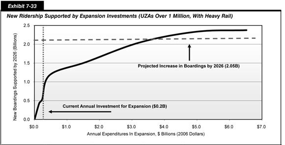
| Average Annual Percent Change vs. 2006 | Average Annual Investment ($B) | New Riders Supported (Billions of Annual Boardings) | Average Annual Growth in Boardings* | Funding Level Description |
|---|---|---|---|---|
| 26.8% | $6.5 | 2.37 | 1.5% | Improve Performance |
| 24.8% | $5.0 | 2.33 | 1.4% | |
| 22.3% | $3.3 | 2.05 | 1.3% | Projected Increase in Boardings by 2026 |
| 15.9% | $1.6 | 1.53 | 1.0% | |
| 6.0% | $0.5 | 1.18 | 0.8% | |
| 0.0% | $0.2 | 0.54 | 0.4% | 2006 Capital Expenditures |
| -4.7% | $0.1 | 0.43 | 0.3% | |
| -50.0% | $0.01 | 0.01 | 0.01% |
To maintain existing performance standards, TERM projects that transit agencies in large cities would need to increase annual capital spending on new assets to an average level of $3.3 billion through 2026. It is estimated that this level of annual expenditure would allow transit agencies to keep pace with the anticipated number of additional annual passenger boardings, forecast to reach a level of 2.05 billion by 2026. This level of new boarding is represented by the horizontal line in the graph in Exhibit 7-33.
To improve performance, TERM estimates that transit operators would need to increase annual capital spending even further. As shown in Exhibit 7-33, projections indicate that annual capital expenditures on expansion projects would need to reach $6.5 billion in order to improve performance, as defined in TERM [see Chapter 8]. This level of spending would allow transit service providers to support 2.37 billion more annual passenger boardings by 2026, a 1.5 percent annual rate of increase in ridership, but may represent an inefficient allocation of resources given the expected 1.2 percent ridership growth in large cities with heavy rail.
Urbanized Areas With Populations of More Than 1 Million Without Heavy Rail Transit Systems
Large metropolitan areas that do not have heavy rail transit systems tend to have newer light rail systems and higher rates of transit ridership growth. These characteristics suggest that transit operators in these cities tend to devote a larger proportion of spending to expansion investments on existing, relatively newer modes of rapid transit, rather than on rehabilitation and replacement projects (as compared to the large, mature transit markets with heavy rail). Key examples of major transit UZAs in this group include Dallas, San Diego, St. Louis, Denver, San Jose, and Sacramento. This section focuses on the impact that rehabilitation and replacement investments, as well as expansion investments, have on transit agencies in these large cities without existing heavy rail modes.
Rehabilitation and Replacement Investments
Exhibit 7-34 displays the effect that rehabilitation and replacement expenditures are expected to have on the future condition of transit assets located in urbanized areas with population of more than 1 million but without heavy rail transit investments.
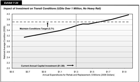
| Average Annual Percent Change vs. 2006 | Average Annual Investment ($B)1 | Average Transit Conditions in 20262 Asset Categories Guideway |
Average Transit Conditions in 20262 Asset Categories Facilities |
Average Transit Conditions in 20262 Asset Categories Systems |
Average Transit Conditions in 20262 Asset Categories Stations |
Average Transit Conditions in 20262 Asset Categories Vehicles |
Average Transit Conditions in 20262 All Transit Assets |
Funding Level Description |
|---|---|---|---|---|---|---|---|---|
| 3.6% | $2.0 | 4.58 | 3.77 | 3.94 | 4.02 | 3.54 | 3.97 | Replace at Condition 3.00 |
| 2.6% | $1.7 | 4.49 | 3.46 | 3.88 | 3.80 | 3.43 | 3.80 | Improve Conditions |
| 1.7% | $1.6 | 4.22 | 3.46 | 3.86 | 3.79 | 3.33 | 3.71 | Maintain Conditions |
| 0.9% | $1.5 | 4.19 | 3.25 | 3.78 | 3.75 | 3.29 | 3.63 | |
| 0.4% | $1.4 | 4.50 | 3.09 | 3.68 | 3.86 | 3.13 | 3.63 | Replace at Condition 2.50 |
| 0.0% | $1.3 | 4.15 | 3.18 | 3.77 | 3.74 | 3.18 | 3.59 | 2006 Capital Expenditures |
| -0.7% | $1.2 | 4.11 | 3.15 | 3.74 | 3.73 | 3.09 | 3.50 | |
| -1.9% | $1.1 | 4.02 | 3.07 | 3.17 | 3.72 | 3.06 | 3.39 | |
| -7.4% | $0.7 | 3.77 | 2.87 | 3.12 | 3.63 | 2.65 | 3.14 |
The level of capital spending dedicated to rehabilitating and replacing assets in 2006 in large cities without heavy rail transit systems was $1.3 billion. This is depicted by the vertical line in the graph in Exhibit 7-34. Note that this level of funding is significantly less than the $6.5 billion of capital spending devoted to rehabilitation and replacement in large cities with heavy rail operators. This difference reflects the significantly larger proportion of investment in existing transit assets in those UZAs with heavy rail versus those without heavy rail.
Future condition ratings for transit assets in these areas, as shown in the exhibit, are projected to decline from the current level of 3.71 to reach 3.59 in 2026 assuming that the current level of annual capital spending on rehabilitation and replacement investments were to continue through 2026.
To maintain conditions in large metropolitan areas without heavy rail service, transit operators are projected to need to increase spending to an average annual level of $1.6 billion through 2026. This level of capital spending is projected to allow the average condition rating of all transit assets to be maintained at 3.71 by 2026, as depicted by the horizontal line in the graph in Exhibit 7-34.
To improve the conditions to those defined by TERM's improve conditions scenario (as defined in Chapter 8), it is estimated that annual capital spending by transit agencies would need to increase to $1.7 billion annually or $0.4 billion above their level in 2006. Under this annual funding scenario, TERM forecasts that the average condition rating for all transit assets would increase to 3.80 by 2026.
Expansion Investments
Exhibit 7-35 shows how the level of annual spending on new assets impacts the number of new passenger boardings that transit agencies in this UZA group would be able to support by 2026. In 2006 transit agencies in these urban areas spent an estimated $2.0 billion on expansion investments. This level of annual capital spending, shown by the vertical line on the graph in Exhibit 7-35, is projected to support an estimated 1.01 billion additional passenger boardings if this level of spending is maintained through 2026. This current level of expenditures is higher than the estimated $0.7 billion in annual investment required to support the expected number of new riders as forecast by the Nation's MPOs (represented by the horizontal line on the graph) and is equal to the estimated $2.0 billion in annual expenditures required to improve performance for this UZA group as defined by TERM's improve performance scenario [see Chapter 8]. This may represent an inefficient allocation of resources given expected ridership growth rates.
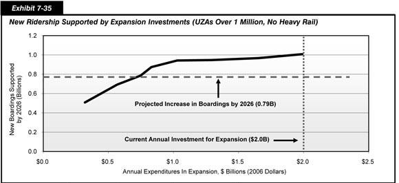
| Average Annual Percent Change vs. 2006 | Average Annual Investment ($2006 B) | New Riders Supported (Billions of Annual Boardings) | Average Annual Growth in Boardings* | Funding Level Description |
|---|---|---|---|---|
| 0.0% | $2.0 | 1.01 | 2.6% | Improve Performance & 2006 Capital Expenditures |
| -1.8% | $1.7 | 0.97 | 2.6% | |
| -4.3% | $1.3 | 0.95 | 2.5% | |
| -6.8% | $1.0 | 0.94 | 2.5% | |
| -9.3% | $0.8 | 0.87 | 2.4% | |
| -10.6% | $0.7 | 0.79 | 2.2% | Projected Increase in Boardings by 2026 |
| -14.3% | $0.6 | 0.69 | 2.0% | |
| -23.6% | $0.3 | 0.51 | 1.5% |
Urbanized Areas With Populations of Less Than 1 Million
Rail transit seldom exists in metropolitan areas that have fewer than 1 million people. These areas are primarily served by transit agencies that operate motor bus services. When compared to the other two metropolitan area groupings analyzed in this section of the chapter, the cities in this segment are dominated by a large number of small to mid-size bus transit agencies and furthermore include many very small operators located in small urban and rural environments. Examples of the larger UZAs in this group include Hartford, Louisville, Richmond, Omaha, and Dayton.
Rehabilitation and Replacement Investments
Exhibit 7-36 illustrates the impact of varying levels of annual rehabilitation and replacement investments on future conditions at transit agencies operating in urbanized areas with populations of less than 1 million. As shown by the vertical line in the graph, annual capital expenditures were $0.7 billion in 2006. TERM projects that if transit agencies in small cities continue to invest at this pace, the average condition rating of assets in 2026 would be 2.70, well below their current average condition rating of 3.72. With the exception of guideway and stations, all asset types would remain between poor or adequate condition, as defined in Chapter 3.
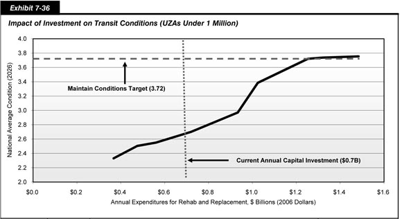
| Average Annual Percent Change vs. 2006 | Average Annual Investment ($B)1 | Average Transit Conditions in 20262 Asset Categories Guideway |
Average Transit Conditions in 20262 Asset Categories Facilities |
Average Transit Conditions in 20262 Asset Categories Systems |
Average Transit Conditions in 20262 Asset Categories Stations |
Average Transit Conditions in 20262 Asset Categories Vehicles |
Average Transit Conditions in 20262 All Transit Assets |
Funding Level Description |
|---|---|---|---|---|---|---|---|---|
| 6.5% | $1.5 | 4.72 | 3.80 | 3.78 | 3.96 | 3.57 | 3.75 | Replace at Condition 3.00 |
| 5.5% | $1.3 | 4.71 | 3.80 | 3.78 | 3.96 | 3.49 | 3.74 | Improve Conditions |
| 5.0% | $1.3 | 4.66 | 3.80 | 3.78 | 3.96 | 3.38 | 3.72 | Maintain Conditions |
| 3.3% | $1.0 | 4.64 | 3.46 | 3.82 | 4.04 | 3.25 | 3.38 | Replace at Condition 2.5 |
| 2.4% | $0.9 | 4.00 | 2.55 | 2.96 | 3.67 | 3.27 | 2.97 | |
| 0.0% | $0.7 | 3.98 | 2.43 | 2.96 | 3.65 | 2.89 | 2.70 | 2006 Capital Expenditures |
| -2.5% | $0.6 | 3.96 | 2.40 | 2.96 | 3.62 | 2.42 | 2.55 | |
| -4.0% | $0.5 | 3.96 | 2.39 | 2.84 | 3.48 | 2.26 | 2.50 | |
| -6.9% | $0.4 | 3.85 | 2.29 | 2.77 | 3.26 | 1.88 | 2.33 |
Conversely, to maintain current conditions through the year 2026, TERM predicts that this group of transit agencies would need to expend roughly $1.3 billion on an annual basis. This amount of investment, as shown by the horizontal line in the graph in Exhibit 7-36, is predicted to allow condition ratings at transit agencies in small cities to remain at 3.72. Under this funding scenario, transit assets in all asset categories would remain between adequate and good condition in 2026.
For conditions at these transit agencies to improve by 2026 (as defined by TERM's "improve performance scenario"), capital expenditures on rehabilitation and replacement activities would need to increase to $1.32 billion from the current spending level of $0.7 billion. This amount of investment would allow the average transit condition rating to improve to 3.74.
Expansion Investments
Similar to other regions of the country, metropolitan areas with populations of less than 1 million are expected to experience increases in transit ridership by 2026. In light of this growth in demand, transit agencies will need to invest in additional assets in order to maintain the existing performance levels of their systems. Specifically, the projected rate of increase in ridership for this group of UZAs averages 1.7 percent, which is significantly higher than the 1.3-percent rate of increase projected for large UZAs with heavy rail but well below the 2.2 percent rate of increase projected for the larger UZAs without existing heavy rail investment.
Exhibit 7-37 shows the impact that annual capital expenditures in expansion investments have on the number of additional annual boardings supported by 2026. As shown by the vertical line in the graph, transit agencies in small urbanized areas, as modeled in TERM, spent an estimated $0.1 billion on expansion investments in 2006. If capital spending continued at this pace, transit agencies in this UZA group would be able to support an additional 0.12 billion boardings in 2026 (an average annual rate of increase of 0.5 percent).
| Average Annual Percent Change vs. 2006 | Average Annual Investment ($B) | New Riders Supported (Billions of Annual Boardings) | Average Annual Growth in Boardings* | Funding Level Description |
|---|---|---|---|---|
| 23.0% | $1.2 | 0.65 | 2.5% | Improve Performance |
| 18.5% | $0.7 | 0.62 | 2.4% | |
| 13.0% | $0.3 | 0.41 | 1.7% | Projected Increase in Boardings by 2026 |
| 9.3% | $0.2 | 0.30 | 1.3% | |
| 4.6% | $0.1 | 0.20 | 0.9% | |
| 2.1% | $0.1 | 0.15 | 0.7% | |
| 0.0% | $0.1 | 0.12 | 0.5% | 2006 Capital Expenditures |
| -1.7% | $0.1 | 0.11 | 0.5% | |
| -3.6% | $0.0 | 0.07 | 0.3% | |
| -9.2% | $0.0 | 0.04 | 0.2% | |
| -14.5% | $0.0 | 0.02 | 0.1% |
Demand for transit services in these small urbanized areas, is expected to increase by 0.41 billion boardings by 2026 (or 1.7 percent annually). To have adequate capacity to support this higher number of riders, transit agencies would need to increase capital spending on expansion investments threefold to $0.3 billion, an amount represented by the horizontal line in the graph in Exhibit 7-37. To improve performance in line with TERM's "improve performance" scenario, transit agencies would need to accelerate the pace of annual capital spending to $1.2 billion annually through 2026, or approximately 12 times the amount spent in 2006; however, this may represent an inefficient allocation of resources given projected ridership increases for small cities and rural areas.
Comparison
The layout and content of Part II of this edition of the C&P report, including Chapters 7 through 10, has been restructured significantly relative to that of recent editions. Much of the material presented in this chapter represents extensions to more limited analyses presented in Chapters 9, 11, and 12 of the 2006 C&P Report. This material is presented earlier in this edition of the report to describe the set of analytical building blocks upon which the selected capital investment scenarios presented in Chapter 8 were developed, and to emphasize the fact that these scenarios represent only selected points on a broad continuum of possible future investment levels.
Exhibits 7-38 and 7-39 provide a crosswalk between the information presented in the exhibits located in the highway and transit sections of this chapter, respectively, and the location of comparable information in the 2006 C&P Report.
Highways and Bridges
As discussed in the highway section of this chapter, the Highway Economic Requirements System (HERS) model has been modified to allow the exploration of linkages between different types of financing mechanisms used to generate revenues for highway investment, and the relationship between alternative investment levels and future system performance.
The Highway section of this chapter examines three broad types of financing mechanisms: those involving non-user sources (such as property taxes or general governmental revenues), fixed rate user charges (such as a vehicle miles traveled [VMT] charge or fuel tax), and variable rate user charges (such as congestion pricing). The bulk of the analyses in the 2006 edition focused primarily on fixed rate user financing mechanisms; the non-user and variable-rate user financing options were addressed as sensitivity analyses in Chapter 10 of the 2006 C&P Report.
Exhibit 7-1 relates the capital expenditure information presented in Chapter 6 to the types of improvements evaluated in the HERS and the National Bridge Investment Analysis System (NBIAS) models. Exhibit 7-2 describes the assumptions made in terms of the ramping up or down of spending levels on a year-by-year basis. Exhibits 7-3 and 7-4 identify the difference between current spending and the alternative levels of future combined public and private spending that were analyzed, and identify changes in fixed rate user charges or variable rate user charges that would align revenues with these spending levels.
Exhibits 7-5 through 7-13 compare the potential impacts of alternative spending levels on a variety of conditions and performance measures on a systemwide basis as computed by HERS. This information is comparable to that presented on a more limited basis in Chapter 9 of the 2006 C&P Report. Exhibit 7-14 provides a funding level description that summarizes why specific funding levels were selected for analysis, and identifies the minimum benefit-cost ratios associated with each of these levels.
Exhibits 7-15 through 7-17 compare the potential impacts of alternative spending levels on a variety of National Highway System (NHS) conditions and performance measures as computed by HERS; Exhibits 7-18 through 7-20 present comparable values for the Interstate system. The 2006 C&P Report included this type of information in Chapter 12 for rural and urban portions of the NHS, and in Chapter 11 for rural and urban portions of the Interstate system.
| Chapter 7 Exhibit | Location of Comparable Information in the 2006 C&P Report |
|---|---|
| Exhibit 7-1 | No direct equivalent for base year spending. Similar information for Investment scenarios shown in Exhibit 7-5. |
| Exhibit 7-2 | No direct equivalent. |
| Exhibit 7-3 | No direct equivalent. |
| Exhibit 7-4 | No direct equivalent. |
| Exhibit 7-5 | "Fixed Rate User Charges" values are comparable to information shown in Exhibit 9-4. |
| Exhibit 7-6 | No direct equivalent. Similar information for VMT growth rates presented in Exhibit 9-7. |
| Exhibit 7-7 | "Fixed Rate User Charges" values are comparable to information shown in Exhibit 9-4. |
| Exhibit 7-8 | "Fixed Rate User Charges" values are comparable to information shown in Exhibit 9-3. |
| Exhibit 7-9 | "Fixed Rate User Charges" values are comparable to information shown in Exhibit 9-3. |
| Exhibit 7-10 | "Fixed Rate User Charges" values are comparable to information shown in Exhibit 9-2. |
| Exhibit 7-11 | "Fixed Rate User Charges" values are comparable to information shown in Exhibit 9-2. |
| Exhibit 7-12 | "Fixed Rate User Charges" values are comparable to information shown in Exhibit 9-1. |
| Exhibit 7-13 | "Fixed Rate User Charges" values are comparable to information shown in Exhibit 9-1. |
| Exhibit 7-14 | No direct equivalent. Benefit-cost ratios discussed in Appendix A (page A-3). |
| Exhibit 7-15 | No direct equivalent. Similar information for rural NHS and urban NHS presented in Exhibits 12-13 and 12-15. |
| Exhibit 7-16 | No direct equivalent. Similar information for rural NHS and urban NHS presented in Exhibits 12-13 and 12-15. |
| Exhibit 7-17 | No direct equivalent. Similar information for rural NHS and urban NHS presented in Exhibits 12-12 and 12-14. |
| Exhibit 7-18 | No direct equivalent. Similar information for rural Interstate and urban Interstate presented in Exhibits 11-16 and 11-18. |
| Exhibit 7-19 | No direct equivalent. Similar information for rural Interstate and urban Interstate presented in Exhibits 11-16 and 11-18. |
| Exhibit 7-20 | No direct equivalent. Similar information for rural Interstate and urban Interstate presented in Exhibits 11-15 and 11-17. |
| Exhibit 7-21 | Comparable to information shown in Exhibit 9-8. |
| Exhibit 7-22 | Comparable to information shown in Exhibit 12-16. |
| Exhibit 7-23 | Comparable to information shown in Exhibit 11-19. |
Exhibits 7-21, 7-22, and 7-23 compare the potential impacts of alternative spending levels on the backlog of economic bridge investments as computed by NBIAS for all bridges, NHS bridges, and Interstate bridges, respectively. Comparable statistics were presented in Chapter 9, Chapter 12, and Chapter 11 of the 2006 C&P Report.
Transit
The transit section of this chapter focuses primarily on how different types and levels of annual capital investments may impact conditions and performance by 2026. Much of the information presented has no direct equivalent in the 2006 C&P Report.
Exhibit 7-24 provides the 2006 actual transit capital expenditures of $12.8 billion as they correspond to the investment scenarios modeled in TERM as a basis for the analysis throughout the chapter.
| Chapter 7 Exhibit | Location of Comparable Information in the 2006 C&P Report |
|---|---|
| Exhibit 7-24 | No direct equivalent. Based on partial data presented in Exhibit 7-8 and 7-9. |
| Exhibit 7-25 | No direct equivalent. |
| Exhibit 7-26 | No direct equivalent. |
| Exhibit 7-27 | No direct equivalent. |
| Exhibit 7-28 | No direct equivalent. |
| Exhibit 7-29 | No direct equivalent. |
| Exhibit 7-30 | No direct equivalent. |
| Exhibit 7-31 | No direct equivalent. |
| Exhibit 7-32 | No direct equivalent. |
| Exhibit 7-33 | No direct equivalent. |
| Exhibit 7-34 | No direct equivalent. |
| Exhibit 7-35 | No direct equivalent. |
| Exhibit 7-36 | No direct equivalent. |
| Exhibit 7-37 | No direct equivalent. Similar information for average investment by scenario, mode, and area population provided in Exhibit 7-10. |
Exhibits 7-25 to 7-28 present the impact of systemwide investments modeled by TERM with specific areas of focus. Exhibit 7-25 focuses on the impact of rehabilitation and replacement investments on transit conditions and provides a summary of the impact of differing levels of annual rehabilitation and replacement investments on the future condition of U.S. transit assets. Exhibit 7-26 presents the impact of expansion investments on transit ridership. This exhibit focuses on the annual capital spending on expansion projects required both to maintain current transit performance levels on all systems and to improve performance on systems with high vehicle occupancies and/or with low operating speeds (this scenario is further detailed in Chapter 8). Exhibit 7-27 presents the impact of performance maintenance investments and shows the relationship between investments made to maintain existing performance and new annual passenger boardings supported by those investments by 2026. Finally, Exhibit 7-28 presents the impact of performance improving investments and demonstrates the relationship between annual performance improvement expenditures and new passenger boardings generated by those investments by 2026.
Exhibits 7-29 to 7-38 focus on how different levels of annual capital investment affect urbanized and rural areas differently. Exhibit 7-29 defines the number of urban and rural agencies by urbanized area (UZA) segment. Exhibit 7-30 presents the total passenger miles and projected annual ridership growth by UZA segment. Exhibits 7-29 and 7-30 not only provides context for the remainder of the exhibits in terms of distribution across urban and rural segments, but also delineates urban agencies with heavy rail and those without heavy rail. Three UZA groupings are identified for the remainder of the analyses, including: (1) large metropolitan areas with heavy rail; (2) large metropolitan areas without heavy rail transit systems; and (3) smaller metropolitan and rural areas. Finally, Exhibits 7-32 to 7-37 present the impact of investment on transit conditions and new ridership supported by expansion investments for the three UZA groupings.