

chapter 3
Summary of Current Highway and Bridge Conditions
Condition of Pavements on Federal-aid Highways
Condition of Bridges — Systemwide
Trends in Pavement Ride Quality
Pavement Ride Quality on the National Highway System
Pavement Ride Quality by Functional Classification
Trends in Bridge Structural Deficiencies
Structurally Deficient Bridges by Owner
Structurally Deficient Bridges on the National Highway System
Structurally Deficient Bridges on the STRAHNET
Structurally Deficient Bridges by Functional Classification
Structurally Deficient Bridges by Age
Factors Affecting Pavement and Bridge Performance
Implications of Pavement and Bridge Conditions for Highway Users
Strategies to Achieve State of Good Repair
The Replacement Value of U.S. Transit Assets
Other Bus Assets (Urban Areas)
Rural Transit Vehicles and Facilities
Highway System Conditions
As referenced in the Introduction to Part I, a key feature of the Moving Ahead for Progress in the 21st Century Act (MAP-21) was the establishment of a performance- and outcome-based program, with the objective of having States invest resources in projects that collectively will make progress toward achieving national goals. For infrastructure condition, MAP-21 established a goal to maintain highway assets in a state of good repair.
Although there is broad consensus that the Nation's transportation infrastructure falls short of a state of good repair, no definition of the term has been uniformly accepted for all transportation assets. The condition of some asset types traditionally has been measured using multiple quantitative indicators, which owners of different transportation assets often weight differently during the assessment process. The condition of other assets has been measured using a single qualitative rating, which introduces subjectivity into the assessment process.
As part of its ongoing efforts to encourage the integration of Transportation Performance Management principles into project selection decisions and to implement related provisions in MAP-21, the Federal Highway Administration (FHWA) issued a Notice of Proposed Rulemaking that included a pavement and bridge performance measures rule (PM-2) on January 5, 2015. Some of the information presented in this section is influenced by the proposed performance measures for pavement and bridge condition presented in the Notice of Proposed Rulemaking; future editions of the C&P report will more fully integrate the final measures that emerge from this rulemaking process.
Data Sources
Pavement condition data are reported to FHWA through the Highway Performance Monitoring System (HPMS). Currently, HPMS requires reporting for Federal-aid highways only, which represent about 25 percent of the Nation's road mileage but carry more than 80 percent of the Nation's travel. States are not required to report on roads functionally classified as rural minor collectors, rural local, or urban local, which comprise the remaining 75 percent of the Nation's road mileage.
HPMS contains data on multiple types of pavement distresses. Data on pavement roughness are used to assess the pavement ride quality experienced by highway users. For some functional systems, States can report a general PSR (Pavement Serviceability Rating) value in place of an actual measurement of pavement roughness through the IRI (International Roughness Index). Other measures of pavement distress include pavement cracking, pavement rutting (surface depressions in the vehicle wheel path, generally relevant only to asphalt pavements), and pavement faulting (the vertical displacement between adjacent jointed sections on concrete pavements).
Condition data for all bridges on the Nation's roadways are reported to FHWA through the National Bridge Inventory (NBI). NBI reflects information the States, Federal agencies, and Tribal governments gather during periodic safety inspections of bridges. Most inspections occur once every 24 months. If a structure shows advanced deterioration, the frequency of inspections might increase so that the safety of the structure can be monitored more closely. Based on certain criteria, some bridges that are in satisfactory or better condition might be inspected between 24 and 48 months with prior FHWA approval. Approximately 83 percent of bridges are inspected every 24 months, 12 percent every 12 months, and 5 percent on a maximum 48-month cycle.
Bridge inspectors are trained to inspect bridges based on, as a minimum, the criteria in the National Bridge Inspection Standards. Routine inspections are required for all structures in the NBI database, 473,709 bridges and 133,589 culverts, with a span greater than 20 feet (6.1 meters) located on public roads.
The NBI database contains condition ratings on the three primary components of a bridge: deck, superstructure, and substructure. The bridge deck, supported by the superstructure, is the surface on which vehicles travel. The superstructure transfers the load of the deck and bridge traffic to the substructure, which provides support for the entire bridge. Such ratings are not reported for the culverts represented in the NBI, as culverts are self-contained units typically located under roadway fill, and thus do not have a deck, superstructure, or substructure. For culverts, a general condition rating is applied instead.
Summary of Current Highway and Bridge Conditions
The PM-2 Notice of Proposed Rulemaking proposed classifications of "Good," "Fair," and "Poor" to assess the conditions of pavements and bridges based on combinations of ratings for individual metrics. This chapter does not include statistics for those combinations, but some data are presented for the individual metrics that would factor into computing the statistics. Exhibit 3-1 identifies criteria for "Good," "Fair," and "Poor" classifications for several individual metrics, based in part on the information laid out in the PM-2 Notice of Proposed Rulemaking. This chapter also references an additional term pertaining to pavement ride quality: "Acceptable" ride quality combines the "Good" and "Fair" categories referenced in Exhibit 3-1.
Condition of Pavements on Federal-aid Highways
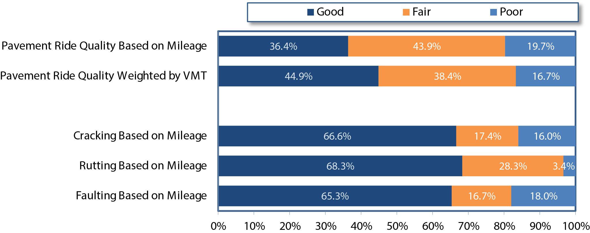
As shown in Exhibit 3-2, approximately 36.4 percent of pavement miles on Federal-aid highways were rated as having good ride quality in 2012, 43.9 percent had fair ride quality, and 19.7 percent had poor ride quality.
When weighted by vehicle miles traveled (VMT) rather than miles of pavement, ride quality appears significantly better. In 2012, approximately 44.9 percent of VMT on Federal-aid highways was on pavements with good ride quality, while only 16.7 percent of VMT on Federal-aid highways was on pavements with poor ride quality. The differences between the mileage-based and VMT-weighted measures imply that, on average, the Nation's roadways with higher traffic volumes have better ride quality than those with lower traffic volumes. This result is positive from a system user perspective, as the VMT-weighted measures better reflect the experience of the individual driver.
Exhibit 3-1 Condition Rating Classifications Used in the 2015 C&P Report |
||||
|---|---|---|---|---|
| Condition Metric | Rating Criteria | Good | Fair | Poor |
| Pavement Ride Quality1 | The International Roughness Index (IRI) measures the cumulative deviation from a smooth surface in inches per mile. | IRI < 95 | IRI 95 to 170 | IRI > 170 |
| Pavement Ride Quality (alternative) | For roads functionally classified as urban minor arterials, rural or urban major collectors, or urban minor collectors, States can instead report a Present Serviceability Rating (PSR) on a scale of 0 to 5. | PSR ≥ 3.5 | PSR ≥ 2.5 and < 3.5 | PSR < 2.5 |
| Pavement Cracking | For asphalt pavements, cracking is measured as the percentage of the pavement surface in the wheel path in which interconnected cracks are present. For concrete pavements cracking is measured as the percent of cracked concrete panels in the evaluated section. | <5% | 5% to 10% | >10% |
| Pavement Rutting (Asphalt Pavements only) | Rutting is measured as the average depth in inches of any surface depression present in the vehicle wheel path. | <0.20 | 0.20 to 0.40 | >0.40 |
| Pavement Faulting (Concrete Pavements only) | Faulting is measured as the average vertical displacement in inches between adjacent jointed concrete panels. | <0.05 | 0.05 to 0.15 | >0.15 |
| Bridge Deck Condition | Ratings are on a scale from 0 "Failed" to 9 "Excellent." | ≥7 | 5 to 6 | ≤4 |
| Bridge Superstructure Condition | Ratings are on a scale from 0 "Failed" to 9 "Excellent." | ≥7 | 5 to 6 | ≤4 |
| Bridge Substructure Condition | Ratings are on a scale from 0 "Failed" to 9 "Excellent." | ≥7 | 5 to 6 | ≤4 |
| Culvert Condition | Ratings are on a scale from 0 "Failed" to 9 "Excellent." | ≥7 | 5 to 6 | ≤4 |
| 1 The PM-2 NPRM sets a different standard for Fair versus Poor ride quality in areas with population over 1 million, setting the break point at 220 rather than 170. This report did not follow this approach, in order to better align with the definition of Acceptable ride quality traditionally used in this report, which includes pavements with IRI values <= 170 inches per mile. | ||||
Exhibit 3-2 Federal-Aid Highway Pavement Conditions, 2012
Source: Highway Performance Monitoring System.
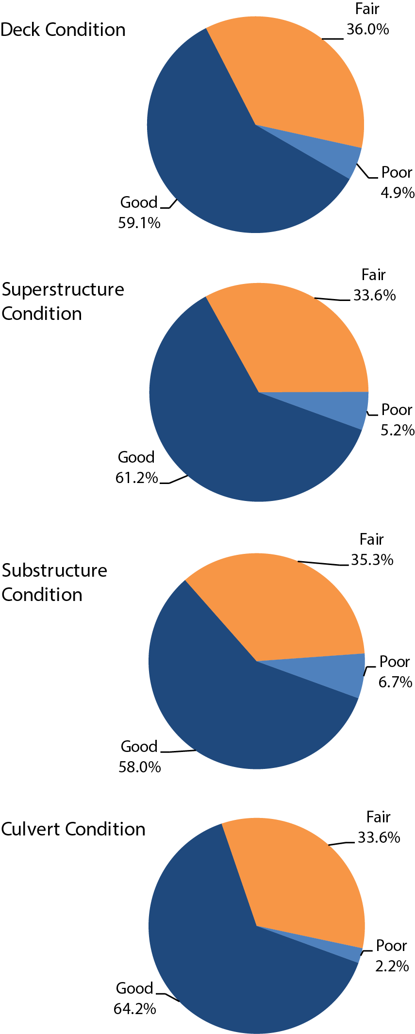
Exhibit 3-3 Bridge and Culvert Conditions, 2012
Source: National Bridge Inventory.
In 2012, approximately 66.6 percent of pavements on Federal-aid highways had good cracking ratings, 68.3 percent had good rutting ratings (where applicable), and 65.3 percent had good faulting ratings (where applicable). Approximately 16.0 percent of pavements on Federal-aid highways had poor cracking ratings, 3.4 percent had poor rutting ratings, and 18.0 percent had poor faulting ratings.
Condition of Bridges — Systemwide
As shown in Exhibit 3-3, the decks of approximately 59.1 percent of bridges were rated as good condition in 2012; 4.9 percent were rated as poor condition. A higher percentage of bridge superstructures had a good rating (61.2 percent ) and a higher percentage was rated as poor (5.2 percent ). Bridge substructures were in the worst condition among the three primary bridge components, with only 58.0 percent rated as good and 6.7 percent rated as poor.
In 2012, approximately 64.2 percent of culverts were rated as good condition, while only 2.2 percent were rated as poor condition. Note that the analyses of future bridge investment presented in Part II of this report exclude culverts; costs associated with culverts are instead indirectly factored into the highway investment analyses.
Trends in Pavement Ride Quality
Exhibit 3-4 details pavement ride quality on Federal-aid highways. The share of pavement mileage with "acceptable" ride quality decreased from 87.4 percent in 2002 to 80.3 percent in 2012. During the same period, the share of miles with pavement ride quality classified as good decreased from 46.6 percent to 36.4 percent .
Between 2008 and 2010, the percentage of pavement mileage with good quality declined from 40.7 percent to 35.1 percent , while the share of mileage with poor ride quality rose from 15.8 percent to 20.0 percent . These results should be interpreted with the understanding that HPMS guidance for reporting IRI changed, beginning with the 2009 data submittal. The revised instructions directed States to include measurements of roughness captured on bridges and railroad crossings; the previous instructions called for such measurements to be excluded from the reported values. This change would tend to increase the measured IRI on average, as the data should now reflect the bump experienced when driving over railroad tracks and the bumpiness associated with open-grated bridges and expansion joints on the bridge decks.
Exhibit 3-4 Pavement Ride Quality on Federal-Aid Highways, 2002—20121 |
||||||
|---|---|---|---|---|---|---|
| 2002 | 2004 | 2006 | 2008 | 2010 | 2012 | |
| By Mileage | ||||||
| Good | 46.6% | 43.1% | 41.5% | 40.7% | 35.1% | 36.4% |
| Fair | 40.8% | 43.6% | 42.7% | 43.5% | 44.9% | 43.9% |
| Acceptable (Good + Fair) | 87.4% | 86.6% | 84.2% | 84.2% | 80.0% | 80.3% |
| Poor | 12.6% | 13.4% | 15.8% | 15.8% | 20.0% | 19.7% |
| Weighted By VMT | ||||||
| Good | 43.8% | 44.2% | 47.0% | 46.4% | 50.6% | 44.9% |
| Fair | 41.6% | 40.7% | 39.0% | 39.0% | 31.4% | 38.4% |
| Acceptable (Good + Fair) | 85.3% | 84.9% | 86.0% | 85.4% | 82.0% | 83.3% |
| Poor | 14.7% | 15.1% | 14.0% | 14.6% | 18.0% | 16.7% |
|
1
Due to changes in data reporting instructions, data for 2010 and beyond are not fully comparable to data for 2008 and prior years.
Source: Highway Performance Monitoring System. |
||||||
Weighting the ride quality data by VMT produces significantly different results. From 2002 to 2012, the share of VMT on Federal-aid highways with acceptable ride quality decreased from 85.3 percent to 83.3 percent , a much smaller decline than that observed above based on mileage. The percentage of Federal-aid highway VMT on pavements with good ride quality rose from 43.8 percent to 44.9 percent .
Although VMT-weighted figures more accurately reflect the typical conditions that highway users would experience over the full length of their trips, focusing on these statistics alone presents an incomplete picture of the current state of Federal-aid highways. The differences between the VMTweighted and mileage-based data clearly suggest that ride quality on those Federal-aid highways that are relatively less traveled has been declining significantly over the past decade. These trends are visible in the data from 2002 to 2008, which predate the 2009 changes to the HPMS guidance, making clear that this finding is not simply a data anomaly but, instead, reflects changes in actual conditions.
Another source of recent data variability is that States have begun reporting ride quality data for shorter section lengths, which would tend to increase the variability of reported ratings. For example, a short segment of pavement in significantly better or worse condition than an adjacent segment is now more likely to be rated as good or poor, whereas before 2009 it might have been averaged with neighboring segments, yielding a rating of fair.
Pavement Ride Quality on the National Highway System
In 1998, the U.S. Department of Transportation (DOT) began establishing annual targets for pavement ride quality. Since 2006, the metric reflected in DOT performance-planning documents has been the share of VMT on pavements within the National Highway System (NHS) having good ride quality. Consequently, the discussion in this section focuses on VMT-weighted measures.
Exhibit 3-5 Percentages of National Highway System Vehicle Miles Traveled on Pavements With Good and Acceptable Ride Quality, 2002—2012 |
||||||
|---|---|---|---|---|---|---|
| 2002 | 2004 | 2006 | 2008 | 20101 | 2012 | |
| Based on NHS before MAP-212 | ||||||
| Good (IRI < 95) | 50% | 52% | 57% | 57% | 60% | |
| Acceptable (IRI ≤ 170) | 91% | 91% | 93% | 92% | 93% | |
| Based on Current NHS | ||||||
| Good (IRI < 95) | 54.7% | 57.1% | ||||
| Acceptable (IRI ≤ 170) | 88.8% | 89.0% | ||||
|
1 Italicized 2010 values shown for the Current NHS are estimates as presented in the 2013 C&P report. Exact values cannot be determined as the 2010 HPMS data were collected based on the pre-MAP-21 NHS. 2 Values are shown as whole percentages to be consistent with how they were reported at the time in DOT performance planning documents. Source: Highway Performance Monitoring System. |
||||||
MAP-21 expanded the NHS to include most of the principal arterial mileage that was not previously included on the system. Although 2012 was the first year for which HPMS data were collected based on this expanded NHS, Exhibit 3-5 includes estimates for 2010 that also were presented in the 2013 C&P Report. As a comparison of the actual 2010 values and these estimates reflects, expanding the NHS reduced the percentage of NHS VMT on pavements with good and acceptable ride quality. On average, the additional routes added to the NHS had rougher pavements than the routes that were already part of the NHS.
From 2010 to 2012, the share of VMT on NHS pavements with acceptable ride quality rose slightly from an estimated 88.8 percent to 89.0 percent . Over the same period, the share of NHS travel on pavements with good ride quality rose from an estimated 54.7 percent to 57.1 percent .
NHS Pavement Ride Quality Trends
Exhibit 3-4 showed that for pavement ride quality on Federal-aid highways, the share of VMT on pavements with good ride quality improved from 2002 to 2012, while the share of mileage with good ride quality declined.
In contrast, the share of pavements with good ride quality for the NHS improved over this period regardless of the weighting method used. Exhibit 3-5 shows that the share of NHS VMT on pavements with good ride quality increased from 50.0 percent in 2002 to 57.1 percent in 2012. This is the metric currently used in DOT performance planning documents.
The share of NHS mileage with good pavement ride quality, however, increased more slowly, from 57.4 percent in 2002 to 59.0 percent in 2012. The share of NHS lane miles with good pavement ride quality increased over this period from 56.7 percent to 59.4 percent . Under the PM-2 Notice of Proposed Rulemaking, pavement-related targets will be set based on lane mileage, rather than mileage or VMT.
Pavement Ride Quality by Functional Classification
Although changes in HPMS reporting procedures in 2009 make identifying trends over the full 10year period shown in Exhibit 3-6 more challenging, drawing some significant conclusions from the data is still possible. Rural Interstates have the best ride quality of all functional systems, with 78.6 percent of VMT on pavements having good ride quality, up from 72.2 percent in 2002. The share of urban Interstate System VMT on pavements with good ride quality from 2002 to 2012 rose sharply from 45.0 percent to 62.5 percent .
Exhibit 3-6 Percentages of Vehicle Miles Traveled on Pavements with Good and Acceptable Ride Quality by Functional System, 2002—2012 |
||||||
|---|---|---|---|---|---|---|
| 2002 | 2004 | 2006 | 2008 | 20101 | 2012 | |
| Functional System | percent Good | |||||
| Rural Interstate | 72.2% | 73.7% | 78.6% | 79.0% | 79.1% | 78.6% |
| Rural Other Freeway and Expressway2 | 74.3% | 72.8% | ||||
| Rural Other Principal Arterial2 | 72.9% | 67.4% | ||||
| Rural Other Principal Arterial2 | 60.2% | 61.0% | 66.8% | 68.4% | ||
| Rural Minor Arterial | 51.0% | 51.5% | 56.3% | 56.2% | 60.9% | 57.7% |
| Rural Major Collector | 42.4% | 40.3% | 39.8% | 39.0% | 41.4% | 39.7% |
| Subtotal Rural | 58.0% | 58.3% | 62.2% | 62.5% | 64.6% | 59.8% |
| Urban Interstate | 45.0% | 49.4% | 54.0% | 55.7% | 64.6% | 62.5% |
| Urban Other Freeway and Expressway | 33.6% | 38.8% | 45.3% | 44.4% | 53.3% | 53.0% |
| Urban Other Principal Arterial | 25.7% | 26.5% | 28.8% | 26.9% | 39.7% | 30.3% |
| Urban Minor Arterial | 34.1% | 32.3% | 33.6% | 32.5% | 28.8% | 22.0% |
| Urban Collector2 | 35.5% | 35.7% | 34.1% | 31.5% | ||
| Urban Major Collector2 | 25.7% | 19.0% | ||||
| Urban Minor Collector2 | 8.6% | 29.8% | ||||
| Subtotal Urban | 34.9% | 36.6% | 39.5% | 38.9% | 44.0% | 36.8% |
| Total Good3 | 43.8% | 44.2% | 47.0% | 46.4% | 50.6% | 44.9% |
| Functional System | percent Acceptable | |||||
| Rural Interstate | 97.3% | 97.8% | 98.2% | 97.3% | 91.1% | 97.6% |
| Rural Other Freeway and Expressway2 | 93.7% | 97.9% | ||||
| Rural Other Principal Arterial2 | 93.0% | 95.9% | ||||
| Rural Other Principal Arterial2 | 96.2% | 96.1% | 97.0% | 97.6% | ||
| Rural Minor Arterial | 93.8% | 94.3% | 95.1% | 94.5% | 87.3% | 93.7% |
| Rural Major Collector | 87.6% | 88.5% | 87.8% | 88.3% | 81.2% | 85.5% |
| Subtotal Rural | 94.1% | 94.5% | 94.9% | 94.8% | 87.8% | 92.8% |
| Urban Interstate | 89.6% | 90.3% | 92.7% | 91.9% | 89.8% | 93.4% |
| Urban Other Freeway and Expressway | 87.8% | 87.7% | 92.1% | 91.4% | 89.2% | 91.9% |
| Urban Other Principal Arterial | 71.0% | 72.6% | 73.8% | 72.4% | 76.4% | 73.5% |
| Urban Minor Arterial | 76.3% | 73.8% | 75.6% | 75.5% | 70.6% | 69.8% |
| Urban Collector2 | 74.6% | 72.6% | 72.6% | 72.0% | ||
| Urban Major Collector2 | 67.0% | 63.8% | ||||
| Urban Minor Collector2 | 26.2% | 59.7% | ||||
| Subtotal Urban | 79.8% | 79.7% | 81.7% | 81.0% | 79.4% | 78.1% |
| Total Acceptable3 | 85.3% | 84.9% | 86.0% | 85.4% | 82.0% | 83.3% |
|
1 HPMS pavement reporting requirements were modified in 2009 to include bridges; features such as open grated bridge decks or expansion joints can greatly increase the IRI for a given section. 2 Beginning in 2010, the data reflect revised HPMS functional classifications. Rural Other Freeways and Expressways were split out of the Rural Other Principal Arterial category, and Urban Collect was split into Urban Major Collector and Urban Minor Collector. 3 Totals shown reflect Federal-aid highways only and exclude roads classified as rural minor collector, rural local, or urban local for which pavement data are not reported in HPMS. Source: Highway Performance Monitoring System. |
||||||
The concept of classification of roadways was presented in Chapter 2. In general, roads with higher functional classifications, which carry higher volumes of traffic at higher speeds such as Interstates and principal arterials, have better ride quality than lower-ordered systems that carry low amounts of traffic, typically at lower speeds, such as collectors. Among the rural functional classifications, the percentage of VMT on pavements with good ride quality in 2012 ranged from 78.6 percent for rural Interstates to 39.7 percent for rural major collectors. A similar pattern is evident among most urban functional classifications, as the percentage of VMT on pavements with good ride quality in 2012 ranged from 62.5 percent for urban Interstates to 19.0 percent for urban major collectors. Urban minor collectors actually showed a higher percentage of VMT on pavements with good ride quality than did urban major collectors in 2012. This observation, however, could derive from the fact that some States have not yet fully adapted to the new functional classifications added to HPMS in 2009, so that the data on urban minor collectors might not be fully representative of the Nation as a whole.
As noted in Chapter 2, rural areas contain about 75 percent of national road miles, but support only about 33 percent of annual national VMT. Pavement conditions in urban areas thus have a greater impact on the VMT-weighted measure shown in Exhibit 3-6 than do pavement conditions in rural areas. Pavement conditions are generally better in rural areas. The share of rural VMT on pavements with good ride quality rose slightly from 58.0 percent in 2002 to 59.8 percent in 2012, while the portion of urban VMT on pavements with good ride quality increased from 34.9 percent in 2002 to 36.8 percent in 2010. The share of VMT on pavements with acceptable ride quality decreased slightly from 2002 to 2012 in rural and urban areas.
Trends in Bridge Structural Deficiencies

Structurally deficient bridges are not unsafe.
Bridges are considered structurally deficient if significant load-carrying elements are in poor condition due to deterioration or damage. They are also considered structurally deficient if the waterway opening of the bridge causes intolerable roadway traffic interruptions.
The classification of a bridge as structurally deficient does not mean that it is likely to collapse or that it is unsafe. Properly scheduled inspections can identify unsafe conditions; if the bridge is determined to be unsafe, the structure is closed. A structurally deficient bridge, when left open to traffic, typically requires significant maintenance and repair and eventual rehabilitation or replacement to address deficiencies. To remain in service, structurally deficient bridges often have lane closures or weight limits that restrict the gross weight of vehicles using the bridges to less than the maximum weight typically allowed by statute.
Bridges are considered structurally deficient if significant load-carrying elements are in poor condition due to deterioration, damage, or both. Structural deficiencies are determined by ratings for a bridge's deck or superstructure, or ratings for culverts. If the load-carrying capacity of a bridge does not meet current design standards and the situation cannot be mitigated through corrective actions short of replacing it, the bridge will be rated as structurally deficient. Bridges over rivers, streams, or channels convey the flow of water so that the roadway is not impacted by flooding. The size of the area or opening under the bridge through which the water is conveyed is a major factor in determining the amount of water that can be passed under the structure. If the size of the structure's hydraulic opening with respect to the passage of water under a bridge does not meet current criteria for potential submersion during a flood event, the bridge will be classified as structurally deficient if bridge replacement is the only option for addressing the situation.
The classification of a bridge as structurally deficient does not imply that the bridge is unsafe. Instead, the classification indicates the extent to which a bridge has deteriorated from its original condition when first built. Once a bridge is classified as structurally deficient, the bridge might experience reduced performance in the form of lane closures or load limits. If a bridge inspection determines a bridge to be unsafe, it is closed.
Exhibit 3-7 identifies the percentages of all bridges classified as structurally deficient based on the number of bridges, bridges weighted by deck area, and bridges weighted by average daily traffic. Chapter 2 provides an overview of growth in the number of bridges over time.
Exhibit 3-7 Structurally Deficient Bridges-Systemwide, 2002—2012 |
||||||
|---|---|---|---|---|---|---|
| 2002 | 2004 | 2006 | 2008 | 2010 | 2012 | |
| Count | ||||||
| Total Bridges | 591,243 | 594,100 | 597,561 | 601,506 | 604,493 | 607,380 |
| Structurally Deficient | 84,031 | 79,971 | 75,422 | 72,883 | 70,431 | 66,749 |
| percent Structurally Deficient | ||||||
| By Bridge Count | 14.2% | 13.5% | 12.6% | 12.1% | 11.7% | 11.0% |
| Weighted by Deck Area | 10.4% | 10.1% | 9.6% | 9.3% | 9.1% | 8.2% |
| Weighted by ADT | 8.0% | 7.6% | 7.4% | 7.2% | 6.7% | 5.9% |
| Source: National Bridge Inventory. | ||||||
Based on raw bridge counts, approximately 11.0 percent of bridges were classified as structurally deficient in 2012-a 3.2-percentage point improvement from the 14.2 percent based on 2002 data. Weighted by deck area, the comparable share was 8.2 percent in 2012, a 2.2-percentage point improvement from 10.4 percent based on 2002 data. Although 11.0 percent of the Nation's bridges are structurally deficient, only 5.9 percent of ADT (average daily traffic) crossed a structurally deficient bridge. ADT measures the total volume of vehicular traffic on a bridge divided by the 365 days in a year.
Structurally Deficient Bridges by Owner
As discussed in Chapter 2, the owner of a road or bridge is responsible for its operation and maintenance. Many local governments have established an interagency agreement with their respective State governments to assume operation and maintenance. Such agreements do not transfer ownership nor do they negate the responsibilities of the bridge owners. Owners must ensure that the operation and maintenance of their bridges comply with Federal and State requirements. Additionally, the National Bridge Inspection Standards specify that each State is responsible for inspecting all bridges in that State except for tribally or federally owned bridges. Similarly, Federal agencies and Tribal governments are responsible for inspecting or causing to be inspected all bridges in their jurisdiction, respectively.
Bridge deficiencies by ownership are examined in Exhibit 3-8. State and local governments own 98.3 percent of the Nation's bridges. Of the relatively few privately owned bridges for which data are reported in NBI-0.2 percent of the total number of bridges-31.6 percent were classified as structurally deficient in 2012. Of the 1.5 percent of bridges Federal agencies own, 7.6 percent were classified as structurally deficient. In terms of structural deficiency, State-owned and locally owned bridges differ significantly, as 7.0 percent of State-owned bridges were structurally deficient in 2012, compared with 14.8 percent of locally owned bridges.
Exhibit 3-8 Structurally Deficient Bridges by Owner, 20121 |
|||||
|---|---|---|---|---|---|
| Federal | State | Local | Private/Other2 | Total | |
| Counts | |||||
| Total Bridges | 8,930 | 292,830 | 304,235 | 1,385 | 607,380 |
| Structurally Deficient Bridges | 679 | 20,531 | 45,101 | 438 | 66,749 |
| Percentages | |||||
| Total Inventory Owned | 1.5% | 48.2% | 50.1% | 0.2% | 100.0% |
| Structurally Deficient Bridges | 7.6% | 7.0% | 14.8% | 31.6% | 11.0% |
|
1 These data only reflect bridges for which inspection data were submitted to the NBI. 2 An unknown number of privately owned bridges are omitted. Source: National Bridge Inventory. |
|||||
Structurally Deficient Bridges on the National Highway System
Exhibit 3-9 identifies the percentage of bridges on the NHS classified as structurally deficient based on the number of bridges, bridges weighted by deck area, and bridges weighted by ADT. The 2012 data shown in the exhibit reflect the NHS before it was expanded under MAP-21. Bridge data for the expanded NHS will be reflected in the next C&P report because MAP-21 was passed in the middle of 2012.
Exhibit 3-9 Structurally Deficient Bridges on the National Highway System, 2002—2012 |
||||||
|---|---|---|---|---|---|---|
| 2002 | 2004 | 2006 | 2008 | 2010 | 2012 | |
| Count | ||||||
| Total Bridges | 114,544 | 115,103 | 115,202 | 116,523 | 116,669 | 117,485 |
| Structurally Deficient Bridges | 6,712 | 6,617 | 6,339 | 6,272 | 5,902 | 5,237 |
| Percentage Structurally Deficient | ||||||
| By Bridge Count | 5.9% | 5.7% | 5.5% | 5.4% | 5.1% | 4.5% |
| Weighted by Deck Area | 8.6% | 8.9% | 8.4% | 8.2% | 8.3% | 7.1% |
| Weighted by ADT | 7.1% | 6.8% | 6.6% | 6.4% | 6.0% | 5.1% |
| Source: National Bridge Inventory. | ||||||
In 2012, approximately 4.5 percent of NHS bridges were classified as structurally deficient. The comparable values weighted by deck area and by ADT were 7.1 percent and 5.1 percent , respectively. These results suggest an above-average concentration of deficiencies on heavily traveled and larger bridges.
FHWA has adopted deck-area weighting for use in agency performance planning in recognition of the significant logistical and financial challenges that might be involved in addressing deficiencies on larger bridges. Between 2002 and 2012, the share of structurally deficient bridges on the NHS weighted by deck area declined from 8.6 percent to 7.1 percent . The 1.2percentage point improvement between 2010 and 2012 was the largest decline during this period.
Structurally Deficient Bridges on the STRAHNET
The STRAHNET (Strategic Highway Network) system is a key subset of NHS. The physical composition of this system was described in Chapter 2, and the condition of the pavement portion was presented earlier in this chapter. The share of structurally deficient bridges decreased from 5.4 percent in 2002 to 4.2 percent in 2012. These data are shown in Exhibit 3-10.
Exhibit 3-10 Structurally Deficient Bridges on the Strategic Highway Network, 2002—2012 |
||||||
|---|---|---|---|---|---|---|
| 2002 | 2004 | 2006 | 2008 | 2010 | 2012 | |
| Total Bridges | 79,852 | 72,046 | 73,003 | 73,771 | 68,529 | 68,118 |
| Structurally Deficient Bridges | 4,320 | 3,640 | 3,645 | 3,659 | 3,355 | 2,890 |
| Percentage of Bridges Structurally Deficient | 5.4% | 5.1% | 5.0% | 5.0% | 4.9% | 4.2% |
| Source: National Bridge Inventory. | ||||||
Structurally Deficient Bridges by Functional Classification
As shown in Exhibit 3-11, the percentage of structurally deficient bridges on the Nation's rural roadways decreased from 15.6 percent in 2002 to 12.3 percent in 2012. Over this same period, the share of structurally deficient bridges on the Nation's urban roadways decreased from 9.5 percent to 7.5 percent .
Exhibit 3-11 Structurally Deficient Bridges by Functional Class, 2002—2012 |
||||||
|---|---|---|---|---|---|---|
| Percentages of Structurally Deficient Bridges by Year | ||||||
| Functional System | 2002 | 2004 | 2006 | 2008 | 2010 | 2012 |
| Rural | ||||||
| Interstate | 4.1% | 4.3% | 4.3% | 4.5% | 4.5% | 4.1% |
| Other Principal Arterial | 5.5% | 5.4% | 5.1% | 4.9% | 4.5% | 3.9% |
| Minor Arterial | 8.7% | 8.4% | 8.3% | 8.1% | 7.3% | 6.6% |
| Major Collector | 12.3% | 11.7% | 11.2% | 10.5% | 10.2% | 9.7% |
| Minor Collector | 14.0% | 13.5% | 12.7% | 12.4% | 12.1% | 11.4% |
| Local | 22.0% | 20.7% | 19.1% | 18.3% | 17.9% | 17.2% |
| Subtotal Rural | 15.6% | 14.8% | 13.9% | 13.3% | 12.9% | 12.3% |
| Urban | ||||||
| Interstate | 6.5% | 6.3% | 6.0% | 5.9% | 5.4% | 4.7% |
| Other Freeway and Expressway | 6.4% | 6.1% | 5.8% | 5.5% | 5.0% | 4.3% |
| Other Principal Arterial | 9.6% | 9.2% | 8.7% | 8.6% | 8.2% | 7.6% |
| Minor Arterial | 10.9% | 10.3% | 10.0% | 9.8% | 9.1% | 8.5% |
| Collector | 11.6% | 11.1% | 11.0% | 10.8% | 9.9% | 9.2% |
| Local | 12.1% | 11.5% | 11.1% | 10.8% | 10.3% | 9.8% |
| Subtotal Urban | 9.5% | 9.1% | 8.8% | 8.6% | 8.1% | 7.5% |
| Total | 14.2% | 13.5% | 12.6% | 12.1% | 11.7% | 11.0% |
| Source: National Bridge Inventory. | ||||||
Among the individual functional classes in 2012, rural local bridges continue to have the highest percentage of structural deficiencies, 17.2 percent . Rural Interstate bridges, however, had the lowest percentage of structural deficiencies, 4.1 percent .
Structurally Deficient Bridges by Age
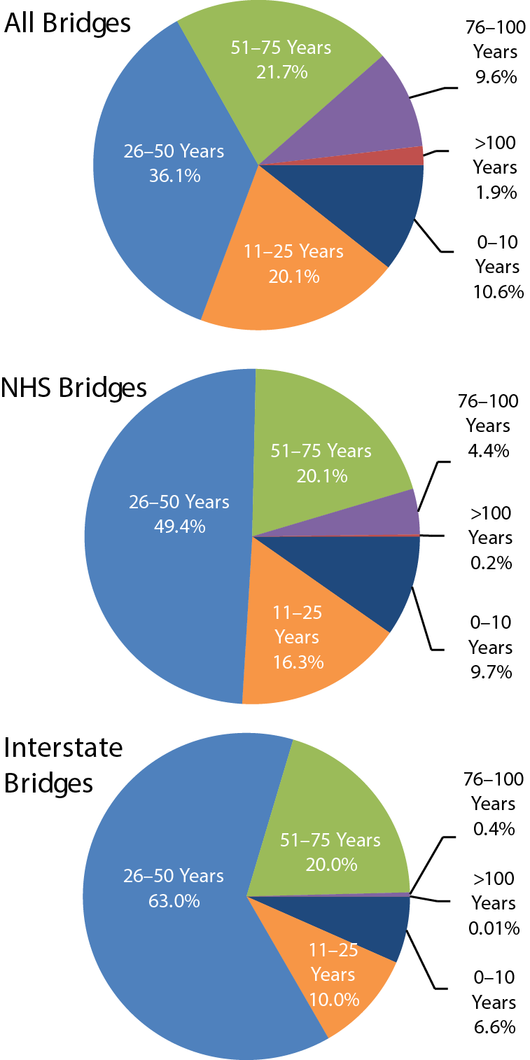
Exhibit 3-12 Bridges by Age, 2012
Source: National Bridge Inventory.
Exhibit 3-12 identifies the age composition of all highway bridges in the Nation. As of 2012, approximately 36.1 percent of the Nation's bridges were between 26 and 50 years old. For NHS bridges, 49.4 percent were in this age range, while 63.0 percent of the Interstate bridges fell into this age range.
Approximately 69.3 percent of all bridges are 26 years old or older. The percentages of NHS and Interstate bridges in this group are 74.0 percent and 83.4 percent, respectively. Most bridges are 26 to 50 years old. The large number of bridges in this age range has implications in terms of long-term bridge rehabilitation and replacement strategies. The need for such actions could be concentrated within certain periods rather than being spread out evenly. Several other variables such as maintenance practices and environmental conditions, however, also influence when future capital investments might be needed.
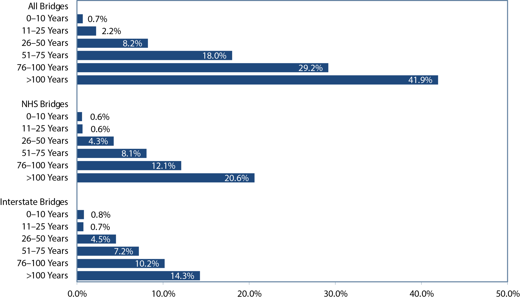
Exhibit 3-13 identifies the distribution of structurally deficient bridges within the age ranges presented in Exhibit 3-12. The percentage of bridges classified as structurally deficient generally tends to rise as bridges age. Although only 8.2 percent of bridges in the 26-to-50 year group are structurally deficient, the percentage is 18.0 percent for bridges 51 to 75 years of age and 29.2 percent for bridges 76 to 100 years of age. Similar patterns are evident in the data for NHS and Interstate System bridges, although the overall percentage of structurally deficient bridges for these systems is lower than for the national bridge population.
The age of a bridge structure is one indicator of its serviceability, or condition under which a bridge is still considered useful. A combination of several factors, however, influences the serviceability of a structure, including the original design; the frequency, timeliness, effectiveness, and appropriateness of the maintenance activities implemented over the life of the structure; the loading to which the structure has been subjected during its life; the climate of the area where the structure is located; and any additional stresses from events such as flooding to which the structure has been subjected. As an example, two structures built at the same time using the same design standards and in the same climate can have very different serviceability levels. The first structure might have had increased heavy truck traffic, lack of preventive maintenance of the deck or the substructure, or lack of rehabilitation work. The second structure could have had the same increases in heavy truck traffic but received timely preventive maintenance activities on all parts of the structure and proper rehabilitation activities. In this example, the first structure would have a low serviceability level, while the second structure would have a high serviceability level.
Exhibit 3-13 Percentages of Structurally Deficient Bridges by Age, 2012
Source: National Bridge Inventory.
Geometric Design Standards
Design standards and best practices for the Nation's roadways have improved over the years. Design standards are intended to improve travel throughout the network by facilitating the movement of passengers and goods through the network. Traveling at higher and safer speeds mitigates congestion and the loss of productivity that occurs from spending more time in a vehicle.
Design standards for both roads and bridges have evolved. Even though standards have improved, however, some facilities have not been updated to meet existing standards. That facilities have been built to lower standards or to outdated standards does not imply that they are poorly maintained.
Roadway Alignment
The term "roadway alignment" refers to the curvature and grade of a roadway, that is, the extent to which it swings from side to side and points up or down. The term "horizontal alignment" relates to curvature (how sharp the curves are), while the term "vertical alignment" relates to gradient (how steep a slope is). Alignment adequacy affects the level of service and safety of the highway system. Inadequate alignment can result in speed reductions and impaired sight distance. Trucks are particularly affected by inadequate vertical alignment with regard to speed. Alignment adequacy is evaluated on a scale from Code 1 (best) to Code 4 (worst).
Exhibit 3-14 Rural Alignment by Functional Class, 20121 |
|||||
|---|---|---|---|---|---|
| Code 1 | Code 2 | Code 3 | Code 4 | ||
| Horizontal | |||||
| Interstate | 85.2% | 0.1% | 1.2% | 13.4% | |
| Other Freeway and Expressway | 63.9% | 1.3% | 1.4% | 33.3% | |
| Other Principal Arterial | 73.2% | 7.9% | 2.7% | 16.3% | |
| Minor Arterial | 69.8% | 4.7% | 2.0% | 23.5% | |
| Major Collector | 68.1% | 1.5% | 0.7% | 29.7% | |
| Vertical | |||||
| Interstate | 86.6% | 11.2% | 1.9% | 0.3% | |
| Other Freeway and Expressway | 79.7% | 17.5% | 1.9% | 1.0% | |
| Other Principal Arterial | 74.2% | 19.1% | 4.4% | 2.3% | |
| Minor Arterial | 67.7% | 19.8% | 8.1% | 4.3% | |
| Major Collector | 90.3% | 6.7% | 0.9% | 2.0% | |
| Code 1 | All curves and grades meet appropriate design standards. | ||||
| Code 2 | Some curves or grades are below design standards for new construction, but curves can be negotiated safely at prevailing speed limits. Truck speed is not substantially affected. | ||||
| Code 3 | Infrequent curves or grades occur that impair sight distance or severely affect truck speeds. May have reduced speed limits. | ||||
| Code 4 | Frequent grades occur that impair sight distance or severely affect truck speeds. Generally, curves are unsafe or uncomfortable at prevailing speed limit, or the speed limit is severely restricted due to the design speed limits of the curves. | ||||
|
1
Values are based on State-reported information and have not been fully validated. The percentage of Horizontal Alignment with Code 4 is significantly higher than that reported in 2008 and prior years. The percentage of Vertical Alignment with Code 1 for Major Collector is also significantly higher than that reported in prior years.
Source: Highway Performance Monitoring System. |
|||||
Alignment adequacy is more important on roads with higher travel speeds or higher volumes (e.g., the Interstate System). Because alignment generally is not a major issue in urban areas, only rural alignment statistics are presented in this section. The amount of change in roadway alignment over time is gradual and occurs only during major reconstruction of existing roadways. New roadways are constructed to meet current vertical and horizontal alignment criteria and, therefore, generally have no alignment problems except under extreme conditions.
As shown in Exhibit 3-14, in 2012, approximately 85.2 percent of rural Interstate System miles are classified as Code 1 for horizontal alignment and 86.6 percent as Code 1 for vertical alignment. In contrast, the percentages of rural minor arterial miles classified as Code 1 for horizontal and vertical alignment, respectively, are only 69.8 percent and 67.7 percent.
Lane Width
Lane width affects capacity and safety. Narrow lanes have less capacity and can affect the frequency of crashes. As with roadway alignment, lane width is more crucial on functional classifications that have higher travel volumes.
Currently, higher functional systems such as the Interstate System are expected to have 12-foot lanes. As shown in Exhibit 3-15, approximately 98.7 percent of rural Interstate System miles and 98.6 percent of urban Interstate System miles had minimum 12-foot lane widths in 2010.
In 2012, approximately 53.8 percent of urban collectors have lane widths of 12 feet or greater, but approximately 18.7 percent have 11-foot lanes and 20.0 percent have 10-foot lanes; the remaining 5.2 percent have lane widths of 9 feet or less. Among rural major collectors, 43.1 percent have lane widths of 12 feet or greater, but approximately 26.1 percent have 11-foot lanes and 22.8 percent have 10 foot lanes. Roughly 6.0 percent of rural major collector mileage has lane widths of 9 feet or less.
Exhibit 3-15 Lane Width by Functional Class, 2012 |
|||||
|---|---|---|---|---|---|
| ≥12 foot | 11 foot | 10 foot | 9 foot | <9 foot | |
| Rural | |||||
| Interstate | 98.7% | 1.2% | 0.1% | 0.0% | 0.0% |
| Other Freeway and Expressway | 97.7% | 2.3% | 0.0% | 0.0% | 0.0% |
| Other Principal Arterial | 91.2% | 6.9% | 1.4% | 0.3% | 0.1% |
| Minor Arterial | 71.6% | 18.9% | 8.5% | 0.8% | 0.2% |
| Major Collector | 43.1% | 26.0% | 22.7% | 6.0% | 2.1% |
| Urban | |||||
| Interstate | 98.6% | 1.0% | 0.3% | 0.1% | 0.0% |
| Other Freeway and Expressway | 95.9% | 3.3% | 0.8% | 0.0% | 0.0% |
| Other Principal Arterial | 82.6% | 12.1% | 4.7% | 0.3% | 0.3% |
| Minor Arterial | 67.0% | 18.5% | 11.7% | 1.8% | 1.0% |
| Collector | 53.8% | 18.7% | 20.0% | 5.2% | 2.4% |
| Source: Highway Performance Monitoring System. | |||||
Functionally Obsolete Bridges
A functionally obsolete bridge is not an unsafe bridge. Functional obsolescence is generally determined by the geometrics of a bridge in relation to the geometrics that current design standards require. In contrast to structural deficiencies, which typically result from deterioration of the bridge components, functional obsolescence generally results from changing traffic demands on the structure. The classification of functionally obsolete is determined by the NBI appraisal ratings for structural evaluation, waterway adequacy, deck geometry, alignment of the approach roadway, and underclearances. Appraisal ratings are used to compare existing characteristics of a bridge to the current standards used for highway and bridge design. Existing bridges constructed before the establishment of more stringent design standards are more likely to be classified functionally obsolete when compared to newer bridges.
Facilities, including bridges, are designed to conform to the design standards in place at the time they are designed. Over time, design requirements improve. For example, a bridge designed in the 1930s would have shoulder widths that conform with 1930s design standards. Current design standards, however, are based on different criteria, and current safety standards require wider bridge shoulders. The difference between the required, current-day shoulder width and the shoulder width designed in the 1930s represents a deficiency. The magnitudes of such deficiencies determine whether a bridge is classified as functionally obsolete.
Of note is whether a bridge has issues that would warrant its classification as both structurally deficient and functionally obsolete. A bridge cannot be classified as both functionally obsolete and structurally deficient. If a functionally obsolete bridge has a structurally deficient component, it is classified as a structurally deficient bridge. To avoid double counting, the standard NBI data reporting convention is to identify it as structurally deficient only. Such bridges are excluded from the statistics on functionally obsolete bridges presented in this section.
Across the system on a national basis, the share of functionally obsolete bridges by bridge count decreased from 15.4 percent in 2002 to 14.0 percent in 2012, as shown in Exhibit 3-16. When considering ADT, the share of functionally obsolete bridges decreased from 22.0 percent in 2002 to 21.3 percent in 2012.
Exhibit 3-16 Functionally Obsolete Bridges-Systemwide, 2002—2012 |
||||||
|---|---|---|---|---|---|---|
| 2002 | 2004 | 2006 | 2008 | 2010 | 2012 | |
| Count | ||||||
| Total Bridges | 591,243 | 594,100 | 597,561 | 601,506 | 604,493 | 607,380 |
| Functionally Obsolete | 90,823 | 90,076 | 89,591 | 89,189 | 85,858 | 84,748 |
| percent Functionally Obsolete | ||||||
| By Bridge Count | 15.4% | 15.2% | 15.0% | 14.8% | 14.2% | 14.0% |
| Weighted by Deck Area | 20.4% | 20.5% | 20.3% | 20.5% | 19.8% | 20.1% |
| Weighted by ADT | 22.0% | 21.9% | 21.9% | 22.2% | 21.5% | 21.3% |
| Source: National Bridge Inventory. | ||||||
Exhibit 3-17 provides the share of functionally obsolete bridges on the NHS. The share of functionally obsolete bridges in NHS based on bridge count decreased from 17.2 percent in 2002 to 16.2 percent in 2012. The share of functionally obsolete bridges based on ADT decreased from 20.0 percent in 2002 to 19.5 percent in 2012.
Exhibit 3-17 Functionally Obsolete Bridges on the National Highway System, 2002—2012 |
||||||
|---|---|---|---|---|---|---|
| 2002 | 2004 | 2006 | 2008 | 2010 | 2012 | |
| Count | ||||||
| Total Bridges | 114,544 | 115,103 | 115,202 | 116,523 | 116,669 | 117,485 |
| Functionally Obsolete | 19,667 | 19,408 | 19,368 | 19,707 | 19,061 | 19,075 |
| percent Functionally Obsolete | ||||||
| By Bridge Count | 17.2% | 16.9% | 16.8% | 16.9% | 16.3% | 16.2% |
| Weighted by Deck Area | 21.1% | 20.9% | 20.8% | 21.4% | 20.3% | 21.0% |
| Weighted by ADT | 20.0% | 19.8% | 20.1% | 20.5% | 19.7% | 19.5% |
| Source: National Bridge Inventory. | ||||||
Most functionally obsolete bridges are located in urban environments. As shown in Exhibit 3-18, urban minor arterials had the highest share of functionally obsolete bridges at 28.2 percent . In the rural setting, Interstate bridges had the highest share of functionally obsolete bridges at 11.6 percent . The disparities between the urban and rural settings could be because urban environments are generally densely populated and have higher traffic volumes.
Exhibit 3-18 Functionally Obsolete Bridges by Functional Class, 2002—2012 |
||||||
|---|---|---|---|---|---|---|
| Functional System | Percentages of Functionally Obsolete Bridges by Year | |||||
| 2002 | 2004 | 2006 | 2008 | 2010 | 2012 | |
| Rural | ||||||
| Interstate | 12.9% | 12.8% | 12.0% | 11.8% | 11.6% | 11.6% |
| Other Principal Arterial | 10.3% | 9.9% | 9.4% | 9.3% | 8.5% | 8.3% |
| Minor Arterial | 12.0% | 11.6% | 11.0% | 10.6% | 10.2% | 9.7% |
| Major Collector | 11.3% | 11.0% | 10.5% | 10.1% | 9.3% | 8.9% |
| Minor Collector | 12.3% | 12.1% | 11.9% | 11.4% | 10.6% | 10.4% |
| Local | 13.5% | 13.2% | 12.8% | 12.4% | 11.7% | 11.3% |
| Subtotal Rural | 12.5% | 12.2% | 11.7% | 11.4% | 10.7% | 10.4% |
| Urban | ||||||
| Interstate | 23.0% | 23.3% | 23.6% | 23.9% | 23.0% | 22.9% |
| Other Freeway and Expressway | 23.5% | 23.2% | 23.1% | 22.9% | 22.0% | 22.1% |
| Other Principal Arterial | 25.4% | 25.4% | 24.5% | 24.5% | 23.8% | 23.4% |
| Minor Arterial | 29.3% | 29.3% | 29.4% | 29.3% | 28.6% | 28.2% |
| Collector | 28.1% | 28.6% | 28.7% | 28.5% | 28.1% | 27.4% |
| Local | 21.4% | 22.0% | 21.9% | 21.4% | 20.5% | 20.7% |
| Subtotal Urban | 24.9% | 25.1% | 25.0% | 24.9% | 24.2% | 24.0% |
| Total | 15.4% | 15.2% | 15.0% | 14.8% | 14.2% | 14.0% |
| Source: National Bridge Inventory. | ||||||
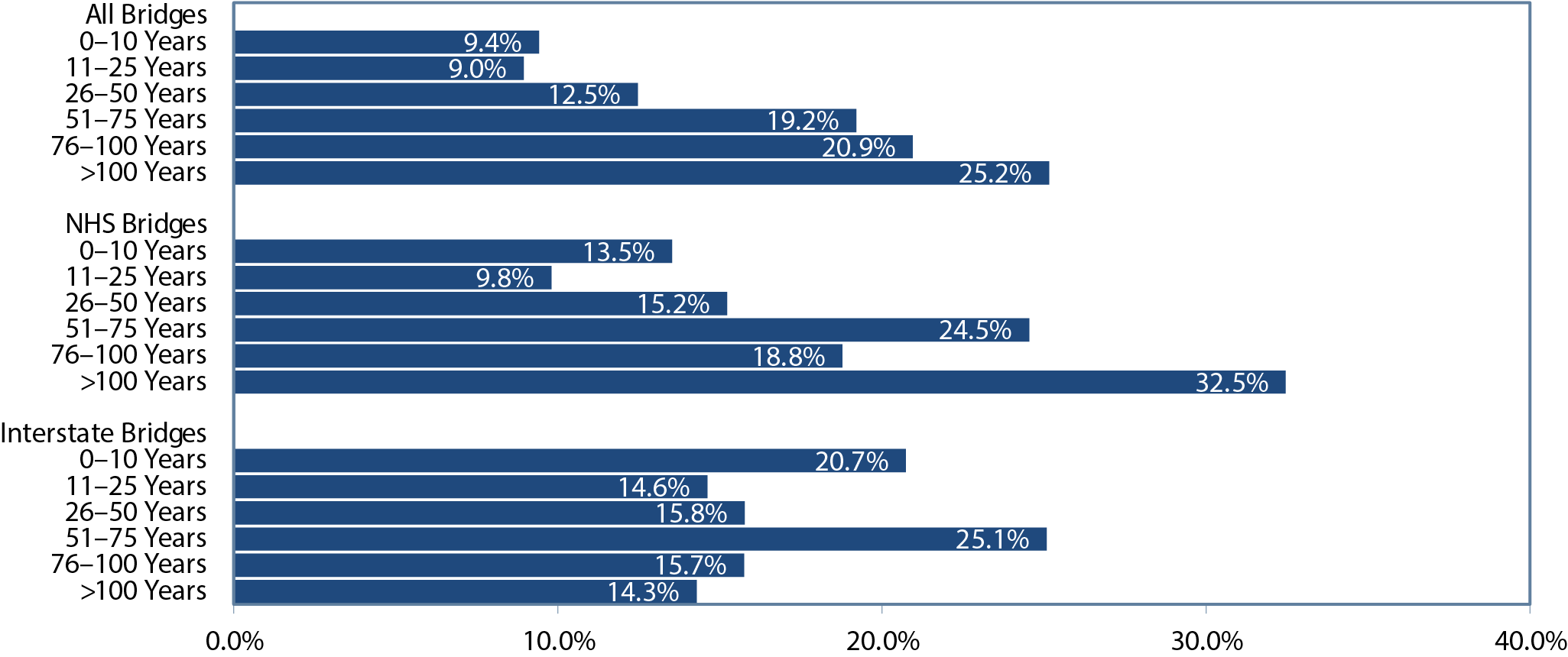
Although bridge design standards have evolved over the past several decades, the standards are not necessarily followed when bridge owners are constructing new bridges. As shown in Exhibit 3-19, 20.7 percent of the functionally obsolete bridges on the Interstate System are between the ages of 0 and 10 years. That portion is the second highest share compared to 25.1 percent of the functionally obsolete bridges on the Interstate System aged 51 to 75 years. Although bridge owners ideally would follow current bridge standards, certain situations might prevent them from completely adhering to the standards.
Exhibit 3-19 Percentages of Functionally Obsolete Bridges by Age, 2012
Source: National Bridge Inventory.
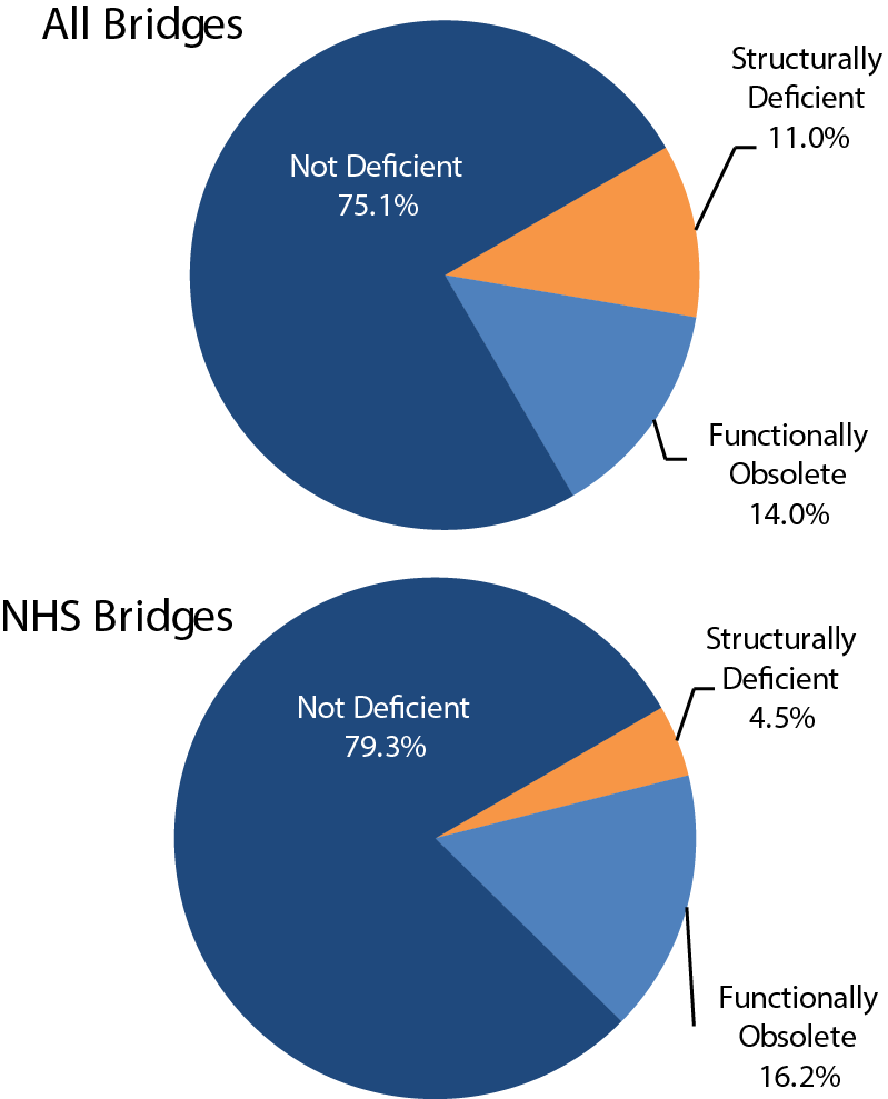
Exhibit 3-20 Bridge Deficiencies: Systemwide vs. National Highway System, 2012
Source: National Bridge Inventory.
Previous editions of the C&P report focused on total bridge deficiencies, combining the structurally deficient bridges with functionally obsolete bridges. Although the number of functionally obsolete bridges remains a concern, FHWA has shifted its focus toward structurally deficient bridges in light of programmatic changes under MAP-21. Consequently, this chapter places greater emphasis on structural deficiencies.
Exhibit 3-20compares the total share of deficient bridges for NHS with all bridges. In 2012, 75.1 percent of the Nation's bridges were not classified as deficient. Approximately 11.0 percent of the Nation's bridges were classified as structurally deficient, and 14.0 percent were classified as functional obsolete, for a total of approximately 24.9 percent deficient.
Among NHS bridges, 79.3 percent were not classified as deficient. Approximately 4.5 percent of NHS bridges were classified as structurally deficient, and 16.2 percent were classified as functionally obsolete, summing to 20.7 percent deficient. Thus, NHS bridges are much less likely to be classified as structurally deficient than non-NHS bridges, but are more likely to be classified as functionally obsolete.
Factors Affecting Pavement and Bridge Performance
Environmental conditions can significantly influence the deterioration of pavements and bridges due to continuous exposure. Pavement and bridge deterioration accelerates on facilities with high traffic volumes. Also, the use of a facility by large numbers of heavy trucks impacts its useful life. Deterioration could be mitigated through reconstruction, rehabilitation, or preventive maintenance. Deterioration can happen rapidly because the impacts of traffic and the environment are cumulative. If no action is taken, deterioration of the pavement and bridges could continue until they can no longer safely support traffic loads.
Constructing new facilities or major rehabilitation is a relatively expensive undertaking. Such actions might not be economically justified until a pavement section or bridge has deteriorated to a poor condition. Such considerations are reflected in the investment scenarios presented in Part II of this report. Those scenarios show that, even if all cost-beneficial investments were made, at any given time a certain percentage of pavements would not meet the criteria for acceptable.
Preventive maintenance actions are less expensive than rehabilitation and can be used to maintain and improve the quality of a pavement section or a bridge. Preventive maintenance actions, however, are less enduring than reconstruction or rehabilitation actions. Preventive maintenance actions are important in extending the useful life of a pavement section or bridge but cannot completely address deterioration over the long term. More aggressive actions would eventually need to be taken to preserve pavement and bridge quality.
Implications of Pavement and Bridge Conditions for Highway Users
Pavement and bridge conditions directly affect vehicle operating costs because deteriorating pavement and bridge decks increase wear and tear on vehicles and repair costs. Poor pavement can also affect travel time costs if road conditions force drivers to reduce speed. Additionally, poor pavement can increase the frequency of crash rates. Highway user costs are discussed in more detail in Chapter 7. Poor bridge conditions could create scenarios in which weight limits force freight trucks to seek alternative routes because they cannot cross a bridge on the most direct route. In worst-case scenarios, a bridge could be closed, forcing all traffic to use alternative routes.
Poor pavement conditions on higher functional classification roadways, such as the Interstate System, tend to result in higher user costs because of vehicle speed. For example, a vehicle hitting a pothole at 55 miles per hour on an Interstate highway could accelerate wear and tear faster than hitting the same pothole at 25 miles per hour.
Although poor pavement and bridge conditions can influence individual users, poor conditions could affect an entire network. Roads with a higher functional classification are meant to facilitate traffic's moving at higher speeds to reduce travel times. Drivers slowing to avoid poor pavement and bridge conditions could create congestion at peak travel times. Congestion increases travel times and slows the movement of freight traffic. The reduction in travel speed would add to the cost of the delivery of goods.
Strategies to Achieve State of Good Repair
Although the Nation's infrastructure system could be rehabilitated to a state of good repair with more investment, FHWA recognizes that stakeholders have limited resources when constructing or repairing roads and bridges. Limited resources-both staff and budgets-at transportation agencies across the country create the need to work more efficiently and focus on technologies and processes that produce the best results.
Improving project delivery continues to be a priority for FHWA. Projects that are delivered faster and more efficiently can minimize the disruption to stakeholders that construction causes. Through the agency's Every Day Counts[1] initiative, FHWA is partnering with State DOTs and stakeholders to identify and rapidly deploy proven but underutilized innovations to shorten the project delivery process, enhance roadway safety, reduce congestion, and improve environmental sustainability.
Bridge replacement projects create considerable traffic disruptions over long periods. Stakeholders might be reluctant to repair or replace a bridge due to its potential impact on traffic. New methodologies enable stakeholders to construct a new bridge off site and perform replacement activities in a consolidated timeframe. Several accelerated bridge construction initiatives are identified below.
Geosynthetic Reinforced SoilIntegrated Bridge System
Defiance County, Ohio, used GRS-IBS to build a bridge in just 6 weeks, compared to the months required for traditional construction methods.The county saved nearly 25 percent on the project, not only because of the reduced labor costs resulting from shorter construction time and simpler construction, but also because fewer materials were required for the GRS bridge abutments. GRS-IBS technology also helped Clearfield County, Pennsylvania, build a bridge on a school bus route in just 35 days, saving months of time and 50 percent on costs. A project to build a bridge built using GRSIBS technology in St. Lawrence County, New York realized a 60 percent cost savings.
1 Federal Highway Administration, Every Day Counts, GRS-IBS Case Studies, www.fhwa.dot.gov/everydaycounts/technology/grs_ibs/casestudies.cfm
2 Randy Albert, Pennsylvania Department of Transportation, "Every Day Counts," EDC Forum, www.fhwa.dot.gov/everydaycounts/forum/post.cfm?id=27
3 Federal Highway Administration, Every Day Counts, GRS-IBS Case Studies, www.fhwa.dot.gov/everydaycounts/technology/grs_ibs/casestudies.cfm
-
Geosynthetic reinforced soil integrated bridge system (GRS-IBS).
Although utilizing traditional equipment and materials, a GRS-IBS makes use of alternating layers of compacted granular fill material and fabric sheets of geotextile reinforcement to provide support. The technology is particularly advantageous in the construction of small bridges (less than 140 feet long), reducing construction time, and generating cost savings of 25 to 60 percent compared to conventional construction methods. It facilitates design flexibility conducive to construction under variable site conditions, including soil type, weather, utilities and other obstructions, and proximity to existing structures.
Prefabricated Bridge Elements and Systems
The Massachusetts DOT used prefabricated bridge elements on a project to replace 14 bridge superstructures on I-93 in Medford, shrinking a 4-year bridge replacement project to just one summer. The agency built the bridge superstructures in sections off site and installed them on weekends during 55-hour windows to minimize impact on travelers.
Prefabricated bridge elements and systems (PBES). With PBES, prefabricated components are constructed off site and moved to the work zone for rapid installation, reducing the level of traffic disruption typically associated with bridge replacement. In some cases, PBES makes removing the old bridge overnight possible, while putting the new bridge in place the next day. Because PBES components are usually fabricated under controlled conditions, weather has less impact on the quality and duration of the project.
In addition to delivering bridge projects faster, FHWA is also delivering pavement innovations to prolong a road's lifespan while providing stakeholders cost savings. These efforts include:
- Intelligent compaction. When pavement cracks prematurely, a potential cause is improper compaction during construction. Intelligent compaction-using global positioning system-based mapping and real-time monitoring to control the compaction process-improves the quality, uniformity, and lifespan of pavements.
- Warm-mix asphalt (WMA). Composed in various fashions, WMA enables construction crews to produce and place asphalt on a road at lower temperatures than is possible using conventional hot-mix methods. In most cases, the lower temperatures result in significant cost savings because fuel consumption during WMA production is typically 20 percent lower. WMA production also generates fewer emissions, making conditions for workers healthier, and can extend the construction season, enabling agencies to deliver projects faster.
-
FHWA launched Every Day Counts (EDC) in cooperation with the American Association of State Highway and Transportation Officials (AASHTO) to speed up the delivery of highway projects and to address the challenges presented by limited budgets. EDC is a State-based model to identify and rapidly deploy proven but underutilized innovations to shorten the project delivery process, enhance roadway safety, reduce congestion, and improve environmental sustainability. EDC-1 occurred in 2011—2012, followed by EDC-2 in 2013—2014, and EDC-3 in 2015—2016. ↑
By cost effectively repairing and replacing roads and bridges with those having longer lifespans, localities can repair or replace a facility to a state of good repair. Stakeholders also will be able to maintain facilities at a high level for a longer period. Localities, in turn, can focus the cost savings from a previous project to other areas of need on the road network
Transit System Conditions
Ideally, the condition and performance of the U.S. transit infrastructure should be evaluated by how well it supports the objectives of the transit agencies that operate it. These objectives include providing safe, fast, cost-effective, reliable, and comfortable service that takes people where they want to go. The degree to which transit service meets these objectives, however, is difficult to quantify and involves trade-offs that are outside the scope of Federal responsibility. This section reports on the quantity, age, and physical condition of transit assets-factors that determine how well the infrastructure can support an agency's objectives and set a foundation for consistent measurement. Transit assets include vehicles, stations, guideway, rail yards, administrative facilities, maintenance facilities, maintenance equipment, power systems, signaling systems, communication systems, and structures that carry elevated or subterranean guideway. Chapter 5 addresses issues relating to the operational performance of transit systems.
Exhibit 3-21 Definitions of Transit Asset Conditions |
||
|---|---|---|
| Rating | Condition | Description |
| Excellent | 4.8—5.0 | No visible defects, near-new condition. |
| Good | 4.0—4.7 | Some slightly defective or deteriorated components. |
| Adequate | 3.0—3.9 | Moderately defective or deteriorated components. |
| Marginal | 2.0—2.9 | Defective or deteriorated components in need of replacement. |
| Poor | 1.0—1.9 | Seriously damaged components in need of immediate repair. |
| Source: Transit Economic Requirements Model. | ||
FTA uses a numerical rating scale ranging from 1 to 5, detailed in Exhibit 3-21, to describe the relative condition of transit assets. A rating of 4.8 to 5.0, or "excellent," indicates that the asset is in nearly new condition or lacks visible defects. The midpoint of the "marginal" rating (2.5) is the threshold below which the assets are considered not in a state of good repair. At the other end of the scale, a rating of 1.0 to 1.9, or "poor," indicates that the asset needs immediate repair and does not support satisfactory transit service.
FTA uses the Transit Economic Requirements Model (TERM) to estimate the condition of transit assets for this report. This model consists of a database of transit assets and deterioration schedules that express asset conditions principally as a function of an asset's age. Vehicle condition is based on the vehicle's maintenance history and an estimate of the major rehabilitation expenditures in addition to vehicle age; the conditions of wayside control systems and track are based on an estimate of use (revenue miles per mile of track) in addition to age. For the purposes of this report, the state of good repair is defined using TERM's numerical condition rating scale. Specifically, this report considers an asset to be in a state of good repair when the physical condition of that asset is at or above a condition rating value of 2.5 (the midpoint of the marginal range). An entire transit system would be in a state of good repair if all of its assets have an estimated condition value of 2.5 or higher. The State of Good Repair benchmark presented in Chapter 8 represents the level of investment required to attain and maintain this definition of a state of good repair by rehabilitating or replacing all assets having estimated condition ratings that are less than this minimum condition value. FTA is currently developing a broader definition of state of good repair to use as a basis for administering MAP-21 grant programs and requirements that are intended to foster better infrastructure reinvestment practices across the industry. This definition might not be the same as the one used in this report.
FTA has estimated typical deterioration schedules for vehicles, maintenance facilities, stations, train control systems, electric power systems, and communication systems through special on-site engineering surveys. Transit vehicle conditions also reflect the most recent information on vehicle age, use, and level of maintenance from the National Transit Database (NTD); the information used in this edition of the C&P report is from 2012. Age information is available on a vehicle-by-vehicle basis from NTD and for all other assets is collected through special surveys. Average maintenance expenditures and major rehabilitation expenditures by vehicle are also available on agency and modal bases. When calculating conditions, FTA assumes agency maintenance and rehabilitation expenditures for a particular mode are the same average value for all vehicles the agency operates in that mode. Because agency maintenance expenditures can fluctuate from year to year, TERM uses a 5-year average.
The deterioration schedules applied for track and guideway structures are based on special studies. Appendix C presents a discussion on the methods used to calculate deterioration schedules and the sources of data on which deterioration schedules are based.
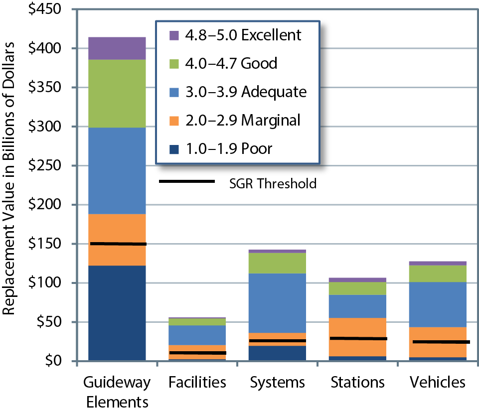
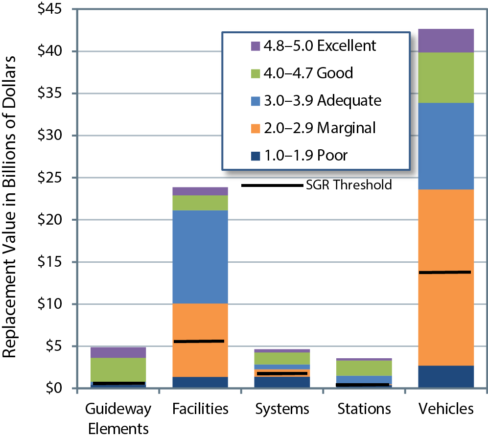
Exhibit 3-22 Distribution of Asset Physical Conditions by Asset Type for All Modes
Source: Transit Economic Requirements Model.
Condition estimates in each edition of the C&P report are based on up-to-date asset inventory information that reflects updates in TERM's asset inventory data. Annual data from NTD were used to update asset records for the Nation's transit vehicle fleets. In addition, updated asset inventory data were collected from 30 of the Nation's largest rail and fixed-route bus transit agencies to support analysis of nonvehicle needs. Because these data are not collected annually, providing accurate time series analysis of nonvehicle assets is not possible. FTA is working to develop improved data in this area. Appendix C provides a more detailed discussion of TERM's data sources. Exhibit 3-22 shows the distribution of asset conditions, by replacement value, across major asset categories for the entire U.S. transit industry.
Condition estimates for assets are weighted by the replacement value of each asset. This weighting accounts for the fact that assets vary substantially in replacement value. For example, a $1-million railcar in poor condition is a much bigger problem than a $1-thousand turnstile in similar condition. To illustrate the calculation involved, consider: The cost-weighted average of a $100 asset in condition 2.0 and a $50 asset in condition 4.0 would be (100 × 2.0 + 50 × 4.0)/(100 + 50) = 2.67. The unweighted average would be (2 + 4)/2 = 3.
The Replacement Value of U.S. Transit Assets
Exhibit 3-23 Estimated Replacement Value of the Nation's Transit Assets, 2012 |
||||
|---|---|---|---|---|
| Transit Asset | Replacement Value (Billions of 2012 Dollars) | |||
| Nonrail | Rail | Joint Assets | Total | |
| Maintenance Facilities | $22.2 | $26.3 | $7.6 | $56.2 |
| Guideway Elements | $7.0 | $406.4 | $1.1 | $414.4 |
| Stations | $3.8 | $102.3 | $0.4 | $106.6 |
| Systems | $4.8 | $133.5 | $4.3 | $142.6 |
| Vehicles | $47.3 | $79.6 | $0.8 | $127.7 |
| Total | $85.1 | $748.1 | $14.2 | $847.5 |
| Source: Transit Economic Requirements Model. | ||||
The total replacement value of the transit infrastructure in the United States for 2012 was estimated at $847.5 billion (in 2102 dollars). These estimates, presented in Exhibit 3-23, are based on asset inventory information in TERM. They exclude the value of assets that belong to special service operators that do not report to NTD. Rail assets totaled $748.1 billion, or roughly 88 percent of all transit assets. Nonrail assets were estimated at $85.1 billion. Joint assets totaled $14.2 billion; joint assets are those that serve more than one mode within a single agency and can include administrative facilities, intermodal transfer centers, agency communications systems (e.g., telephone, radios, and computer networks), and vehicles that agency management uses (e.g., vans and automobiles).
Bus Vehicles (Urban Areas)
Bus vehicle age and condition are reported according to vehicle type for 2002 to 2012 in Exhibit 3-24. When measured across all vehicle types, the average age of the Nation's bus fleet has remained essentially unchanged since 2002. Similarly, the average condition rating for all bus types (calculated as the weighted average of bus asset conditions, weighted by asset replacement value) is also relatively unchanged, remaining near the bottom of the adequate range for the past 10 years. The percentage of vehicles below the state of good repair replacement threshold (condition 2.5) has remained at 10—12 percent for this same period. Note that, although this observation holds across all vehicle types, the proportion of full-size buses (the vehicle type that supports most fixed-route bus services) declined from 15.2 percent in 2008 to 12.3 percent in 2012. This reduction likely reflects impacts of transit-related spending under the American Recovery and Reinvestment Act. The Nation's bus fleet has grown at an average annual rate of roughly 2 percent over the past 10 years, with most of this growth concentrated in three vehicle types: large, 60-foot articulated buses; small buses less than 25 feet long (frequently dedicated to flexible-route bus services); and vans. The large increase in the number of vans reflects both the needs of an aging population (paratransit services) and an increase in the popularity of vanpool services. In contrast, the number of full- and medium-sized buses has remained relatively flat since 2002.
Exhibit 3-24 Urban Transit Bus Fleet Count, Age, and Condition, 2002—2012 |
||||||
|---|---|---|---|---|---|---|
| 2002 | 2004 | 2006 | 2008 | 2010 | 2012 | |
| Articulated Buses | ||||||
| Fleet Count | 2,799 | 3,074 | 3,445 | 4,302 | 4,896 | 5,043 |
| Average Age (Years) | 7.2 | 5.0 | 5.3 | 6.3 | 6.5 | 7.0 |
| Average Condition Rating | 3.3 | 3.5 | 3.5 | 3.3 | 3.2 | 3.1 |
| Below Condition 2.50 (Percent) | 16.6% | 5.0% | 2.1% | 2.6% | 3.7% | 5.3% |
| Full-Size Buses | ||||||
| Fleet Count | 46,573 | 46,139 | 46,714 | 45,985 | 45,441 | 44,906 |
| Average Age (Years) | 7.5 | 7.2 | 7.4 | 7.9 | 7.8 | 8.0 |
| Average Condition Rating | 3.2 | 3.2 | 3.2 | 3.1 | 3.1 | 2.9 |
| Below Condition 2.50 (Percent) | 13.1% | 12.3% | 11.3% | 15.2% | 12.5% | 12.3% |
| Mid-Size Buses | ||||||
| Fleet Count | 7,269 | 7,114 | 6,844 | 7,009 | 7,218 | 7,077 |
| Average Age (Years) | 8.4 | 8.1 | 8.2 | 8.3 | 8.1 | 7.4 |
| Average Condition Rating | 3.1 | 3.1 | 3.1 | 3.1 | 3.1 | 3.0 |
| Below Condition 2.50 (Percent) | 14.1% | 13.2% | 14.2% | 12.4% | 12.5% | 8.2% |
| Small Buses | ||||||
| Fleet Count | 14,857 | 15,972 | 16,156 | 19,366 | 19,493 | 23,793 |
| Average Age (Years) | 4.5 | 4.6 | 5.1 | 5.1 | 5.2 | 5.2 |
| Average Condition Rating | 3.4 | 3.5 | 3.4 | 3.4 | 3.4 | 3.3 |
| Below Condition 2.50 (Percent) | 8.8% | 10.1% | 10.3% | 11.6% | 10.2% | 13.1% |
| Vans | ||||||
| Fleet Count | 17,147 | 18,713 | 19,515 | 26,823 | 28,531 | 28,193 |
| Average Age (Years) | 3.2 | 3.3 | 3.0 | 3.2 | 3.4 | 3.8 |
| Average Condition Rating | 3.7 | 3.8 | 3.8 | 3.8 | 3.7 | 3.6 |
| Below Condition 2.50 (Percent) | 7.2% | 6.7% | 8.4% | 8.0% | 8.2% | 4.1% |
| Total Fixed-Route Bus | ||||||
| Total Fleet Count | 88,645 | 91,012 | 92,674 | 103,485 | 105,579 | 109,012 |
| Weighted Average Age (Years) | 6.2 | 6.0 | 6.0 | 6.1 | 6.1 | 6.2 |
| Weighted Average Condition Rating | 3.2 | 3.3 | 3.3 | 3.1 | 3.0 | 3.2 |
| Below Condition 2.50 (Percent) | 11.8% | 10.6% | 10.4% | 12.0% | 10.5% | 9.8% |
| Sources: Transit Economic Requirements Model and National Transit Database. | ||||||
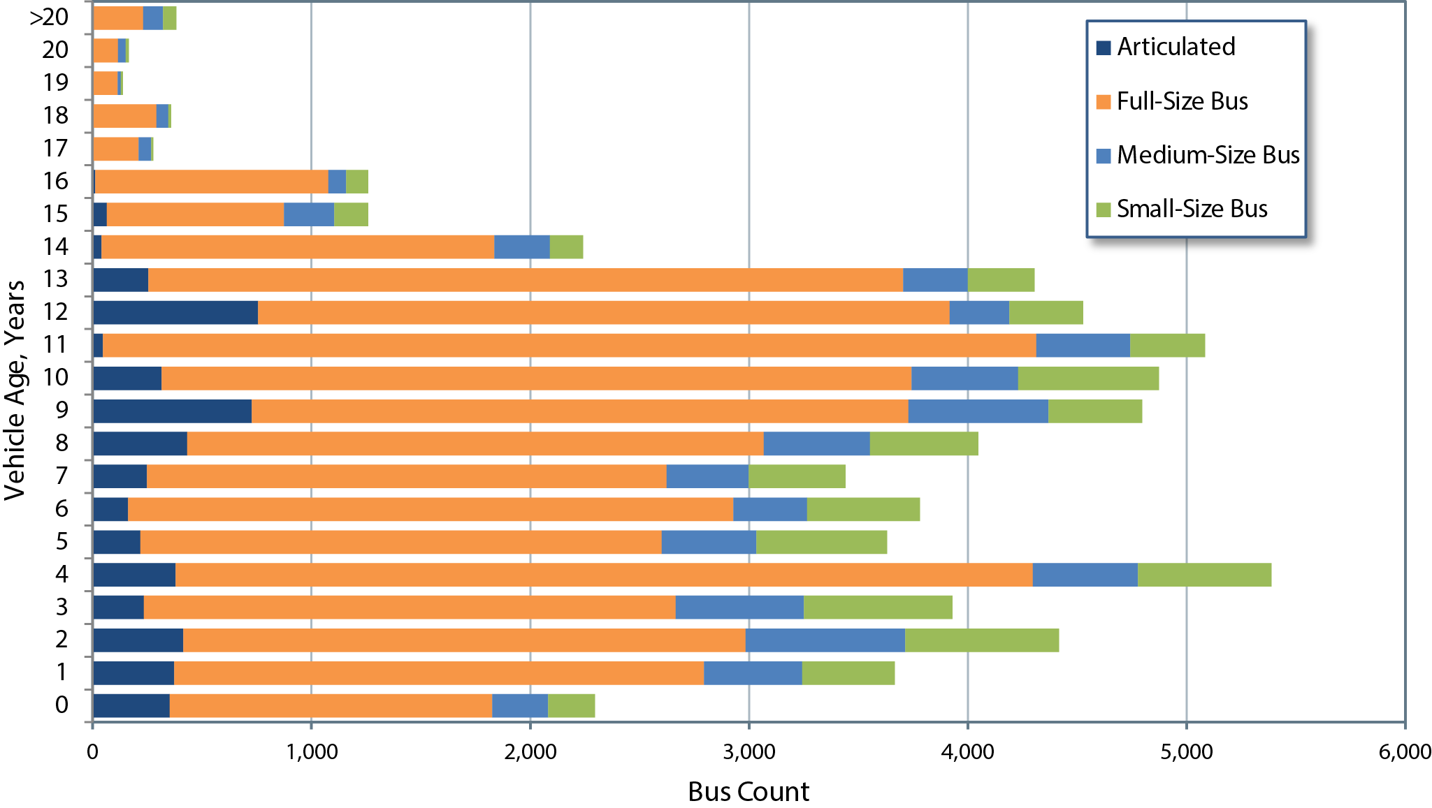
Exhibits 3-25 and 3-26 present the age distribution of the Nation's transit buses and vans, minivans, and autos, respectively. Note here that full-size buses and vans account for the highest proportion (roughly 67 percent ) of the Nation's rubber-tire transit vehicles. Moreover, although most vans are retired by age 7 and most buses by age 15, roughly 5 to 20 percent of these fleets remain in service well after their typical retirement ages.
A distinction should be made between "small buses" and cutaways. By definition, small buses are 30-foot long vehicles operating mostly as fixed route. Cutaways are buses less than 30 feet in length, operating mostly as demand response.
Exhibit 3-25 Age Distribution of Fixed-Route Buses (Urban Areas), 2012
Source: Transit Economic Requirements Model and National Transit Database.
Exhibit 3-26 Age Distribution of Vans, Minivans, Autos, and Cutaways (Urban Areas), 2012
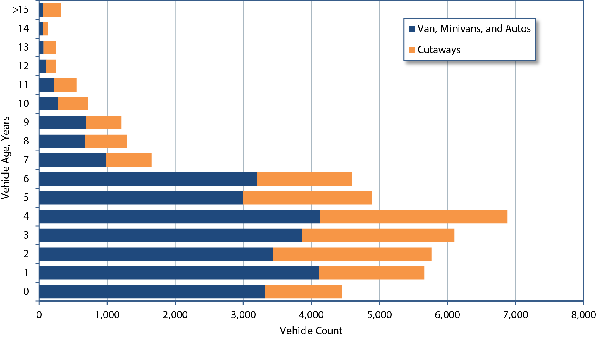
Source: Transit Economic Requirements Model and National Transit Database.
Other Bus Assets (Urban Areas)
Exhibit 3-27 Distribution of Estimated Asset Conditions by Asset Type for Fixed-Route Bus
Source: Transit Economic Requirements Model.
The more comprehensive capital asset data described above enable reporting of a more complete picture of the overall condition of bus-related assets. Exhibit 3-27 shows TERM estimates of current conditions for the major categories of fixed-route bus assets. Vehicles comprise roughly half of all fixed-route bus assets, and maintenance facilities make up another third. Roughly one-third of bus maintenance facilities are rated below condition 3.0, compared to roughly one-half for bus, paratransit, and vanpool vehicles.
Rail Vehicles
NTD compiles annual data on all rail vehicles; these data are shown in Exhibit 3-28, broken down by major category of rail vehicles. Measured across all rail vehicle types, the average age of the Nation's rail fleet has remained essentially unchanged, between 19 and 20 years old, since 2004. The average condition of all rail vehicle types (calculated as the weighted average of vehicle conditions, weighted by vehicle replacement cost) is also relatively unchanged, remaining near 3.5 since 2002. The percentage of vehicles below the state of good repair replacement threshold (condition 2.5) has remained between 3.6 and 4.6 percent since 2002. Note that, although this observation holds across all vehicle types, the analysis suggests that most vehicles in lesser condition occur in the light and heavy rail fleets. Most light rail vehicles with an estimated condition of less than 2.5, however, are historic streetcars and trolley cars with an average age of 75 years. Given their historic vehicle status, the estimated condition of these vehicles (determined primarily by age) should be viewed as a rough approximation.
From 2002 to 2012, the Nation's rail transit fleet grew at an average annual rate of roughly 1.3 percent . This rate of growth was largely due to the rate of increase in the heavy rail fleet (which represents slightly more than half the total fleet and grew at an average annual rate of 0.4 percent over this period). In contrast, the annual rate of increase in commuter rail and light rail fleets has been appreciably higher, averaging approximately 2.1 percent and 3.2 percent , respectively. These higher growth rates reflect recent rail transit investments in small and medium-sized urban areas where the size and population density do not justify the greater investment needed for heavy rail construction.
Exhibit 3-28 Urban Transit Rail Fleet Count, Age, and Condition, 2002—2012 |
|||||||||||
|---|---|---|---|---|---|---|---|---|---|---|---|
| 2002 | 2004 | 2006 | 2008 | 2010 | 2012 | ||||||
| Commuter Rail Locomotives | |||||||||||
| Fleet Count | 709 | 710 | 740 | 790 | 822 | 877 | |||||
| Average Age (Years) | 17.2 | 17.8 | 16.7 | 19.6 | 19.4 | 17.8 | |||||
| Average Condition Rating | 3.7 | 3.7 | 4.0 | 3.6 | 3.6 | 3.7 | |||||
| Below Condition 2.50 (Percent) | 0.0% | 0.0% | 0.0% | 0.0% | 0.0% | 1.8% | |||||
| Commuter Rail Passenger Coaches | |||||||||||
| Fleet Count | 2,985 | 3,513 | 3,671 | 3,539 | 3,711 | 3,758 | |||||
| Average Age (Years) | 19.2 | 17.7 | 16.8 | 19.9 | 19.1 | 20.2 | |||||
| Average Condition Rating | 3.7 | 3.8 | 4.1 | 3.6 | 3.7 | 3.6 | |||||
| Below Condition 2.50 (Percent) | 0.0% | 0.0% | 0.0% | 0.0% | 0.0% | 0.4% | |||||
| Commuter Rail Self-Propelled Passenger Coaches | |||||||||||
| Fleet Count | 2,389 | 2,470 | 2,933 | 2,665 | 2,659 | 2,930 | |||||
| Average Age (Years) | 27.1 | 23.6 | 14.7 | 18.9 | 19.7 | 19.7 | |||||
| Average Condition Rating | 3.5 | 3.7 | 3.8 | 3.7 | 3.7 | 3.6 | |||||
| Below Condition 2.50 (Percent) | 0.0% | 0.0% | 0.0% | 0.0% | 0.0% | 0.0% | |||||
| Heavy Rail | |||||||||||
| Fleet Count | 11,093 | 11,046 | 11,075 | 11,570 | 11,648 | 11,587 | |||||
| Average Age (Years) | 19.8 | 19.8 | 22.3 | 21.0 | 18.8 | 19.9 | |||||
| Average Condition Rating | 3.4 | 3.4 | 3.3 | 3.3 | 3.4 | 3.4 | |||||
| Below Condition 2.50 (Percent) | 6.1% | 5.6% | 5.5% | 6.1% | 5.2% | 3.7% | |||||
| Light Rail1 | |||||||||||
| Fleet Count | 1,637 | 1,884 | 1,832 | 2,151 | 2,222 | 2,241 | |||||
| Average Age (Years) | 17.9 | 16.5 | 14.6 | 17.1 | 18.1 | 14.6 | |||||
| Average Condition Rating | 3.5 | 3.6 | 3.7 | 3.6 | 3.5 | 3.6 | |||||
| Below Condition 2.50 (Percent) | 11.8% | 9.3% | 6.4% | 7.1% | 6.9% | 6.3% | |||||
| Total Rail | |||||||||||
| Total Fleet Count | 18,813 | 19,623 | 20,251 | 20,715 | 21,062 | 21,393 | |||||
| Weighted Average Age (Years) | 20.4 | 19.5 | 19.3 | 20.1 | 18.9 | 19.3 | |||||
| Weighted Average Condition Rating | 3.5 | 3.5 | 3.6 | 3.5 | 3.5 | 3.5 | |||||
| Below Condition 2.50 (Percent) | 4.6% | 4.1% | 3.6% | 4.2% | 3.6% | 2.8% | |||||
|
1
Excludes vintage streetcars. Source: Transit Economic Requirements Model and National Transit Database. |
|||||||||||
Exhibit 3-29 presents the age distribution of the Nation's heavy rail, light rail, and commuter rail transit vehicles. Heavy rail vehicles account for more than half the Nation's rail fleet, whereas light rail, a mode typically found in smaller rail markets, accounts for only 11 percent of rail vehicles. At the same time, roughly one-third of rail and commuter vehicles are more than 25 years old-with close to 3,000 heavy and commuter rail vehicles exceeding 35 years in age. Comparing the results in Exhibit 3-29 with the age distribution of transit buses and vans in Exhibit 3-25 and Exhibit 3-26 is instructive; a comparatively clear pattern of preferred retirement age is evident in the bus and van vehicle type but no such pattern is shown in the rail vehicle results. Exhibit 3-30 presents the age distribution of the Nation's hybrid rail, streetcar, and other rail transit vehicles.
Exhibit 3-29 Age Distribution of Rail Transit Vehicles, 2012
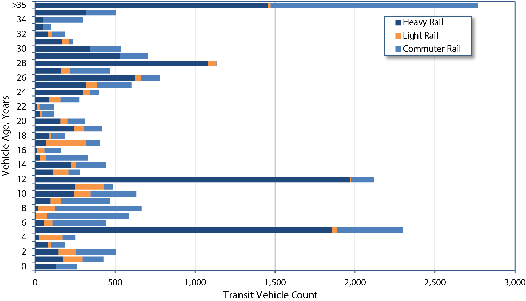
Source: Transit Economic Requirements Model and National Transit Database.
Exhibit 3-30 Age Distribution of Rail Transit Vehicles, 2012
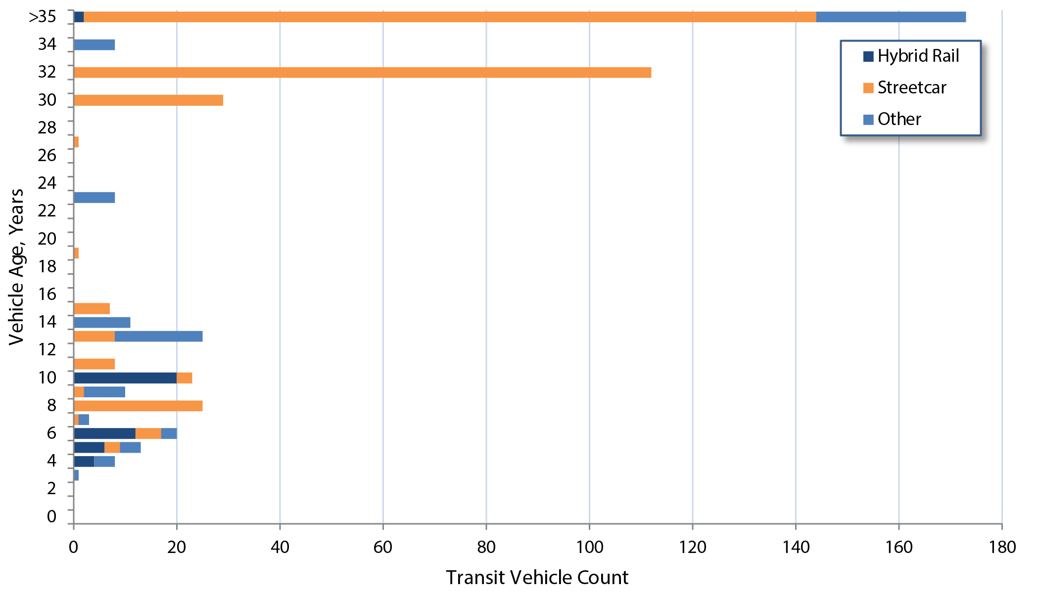
Source: Transit Economic Requirements Model and National Transit Database.
Other Rail Assets
Exhibit 3-31 Distribution of Asset Physical Conditions by Asset Type for All Rail
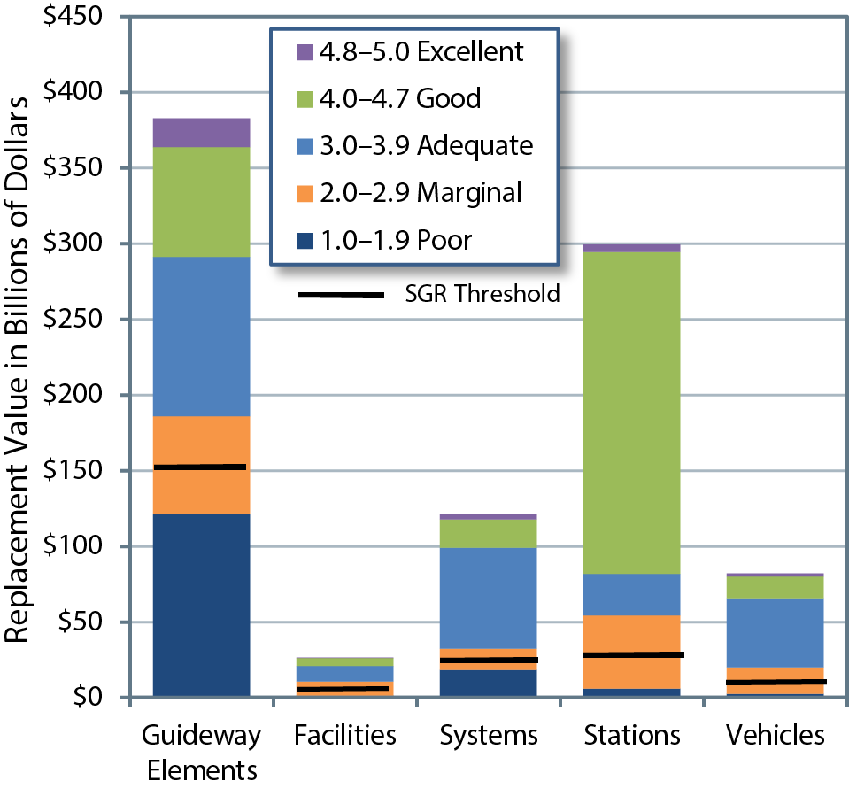
Source: Transit Economic Requirements Model.
Assets associated with nonvehicle transit rail can be divided into four general categories: guideway elements, systems, stations, and facilities. TERM estimates of the condition distribution for each category are shown in Exhibit 3-31.
The largest category by replacement value is guideway elements. These elements consist of tracks, ties, switches, ballasts, tunnels, and elevated structures. The replacement value of this category is $382.8 billion, of which $121.6 billion is rated below condition 2.0 (32 percent ) and $64.1 billion is rated between conditions 2.0 and 3.0. The relatively large proportion of guideway and systems assets rated below condition 2.0 and the magnitude of the $140-billion investment required to replace or keep them in a state of good repair represent major challenges to the transit rail industry.
Although maintaining these assets is among the largest expenses associated with operating rail transit, FTA does not collect detailed data on these elements, in part because the elements are difficult to categorize into discrete sections having common life expectancies. Service life for track, for example, highly depends on the amount of use it receives and its location.
Systems, which consist of power, communication, and train control equipment, have a replacement value of $121.4 billion, of which $18.3 billion is rated below condition 2.0 (15 percent ) and $14 billion is rated between conditions 2.0 and 3.0. This category is another for which many assets are difficult to characterize in terms of standard types and life expectancies. As a result, FTA has only limited data from which to make needs projections.
Stations have a replacement value of $299.3 billion. Only $5.9 billion is rated below condition 2.0 and $48.4 billion is rated between conditions 2.0 and 3.0.
Facilities, principally consisting of maintenance and administration buildings, have a replacement value of $26.4 billion. The value rated below condition 2.0 is $1.3 billion, and between conditions 2.0 and 3.0 is $9.3 billion.
Rail transit consists of heavy rail (urban dedicated guideway), light rail, hybrid rail, streetcar (in mixed traffic), and commuter rail (suburban passenger rail) modes. Almost half of rail transit vehicles are in heavy rail systems. Heavy rail represents $255.2 billion (84 percent ) of the total transit rail replacement cost of $303.2 billion. Heavy rail serves some of the Nation's oldest and largest transit systems (Boston, New York, Washington, San Francisco, Philadelphia, and Chicago).
Exhibit 3-32 Distribution of Asset Physical Conditions by Asset Type for Heavy Rail
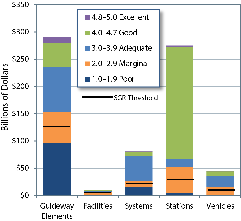
Source: Transit Economic Requirements Model.
The condition distribution of heavy rail assets, which represent the largest share of U.S. rail transit assets, is shown in Exhibit 3-32.
Exhibit 3-33 shows the average age and condition of nonvehicle transit assets for fixed-route bus and rail modes reported for 2012.
While Exhibit 3-31 depicts the replacement value of national transit assets by category for rail modes, Exhibit 3-33 provides additional data such as average fleet age, average condition, and percent of assets below the state of good repair threshold (rating below 2.5).
The data reinforce the analysis of Exhibit 3-23, namely that assets for rail modes represent major challenges to the transit rail industry. For example, the average condition of all rail asset categories is near the upper bound of the marginal rating; 35 percent of guideway elements-the asset category having the highest replacement value-are below a state of good repair. Stations have the largest percentage of assets below a state of good repair, 38 percent .
Exhibit 3-33 Non-Vehicle Transit Assets: Age and Condition, 2012 |
||||
|---|---|---|---|---|
| Category | Mode Type | Average Age | Average Condition | Percent Below Condition 2.5 |
| Facilities | Rail | 35.4 | 3.2 | 24% |
| Fixed-Route Bus | 30.4 | 3.2 | 7% | |
| All | 32.8 | 3.2 | 15% | |
| Guideway Elements | Rail | 64.3 | 3.1 | 35% |
| Fixed-Route Bus | 24.0 | 4.5 | 6% | |
| All | 63.5 | 3.1 | 35% | |
| Stations | Rail | 57.8 | 3.0 | 38% |
| Fixed-Route Bus | 22.9 | 4.0 | 12% | |
| All | 57.3 | 3.0 | 37% | |
| Systems | Rail | 31.6 | 3.3 | 17% |
| Fixed-Route Bus | 23.6 | 3.5 | 17% | |
| All | 31.1 | 3.3 | 17% | |
| Source: Transit Economic Requirements Model. | ||||
Rural Transit Vehicles and Facilities
Rural systems operate buses, vans, or other small passenger vehicles (see Chapter 2). Data on the numbers and ages of rural vehicles and the number of maintenance facilities are now compiled in NTD, enabling FTA to report more accurately on rural transit conditions and on the 727 rural maintenance facilities in 2012. The age distributions of rural transit vehicles for buses and for vans, minivans, autos, and cutaways are summarized in Exhibit 3-34 and Exhibit 3-35, respectively . The relative small average fleet age of fixed-route buses is due to the large proportion of cutaway vehicles, which are usually built based on incomplete vans with added specific equipment required for transit service. These vehicles have 4 to 5 years average useful life and need frequent replacement.
Exhibit 3-34 Age Distribution of Rural Transit Vehicles for Fixed-Route Buses, 2012
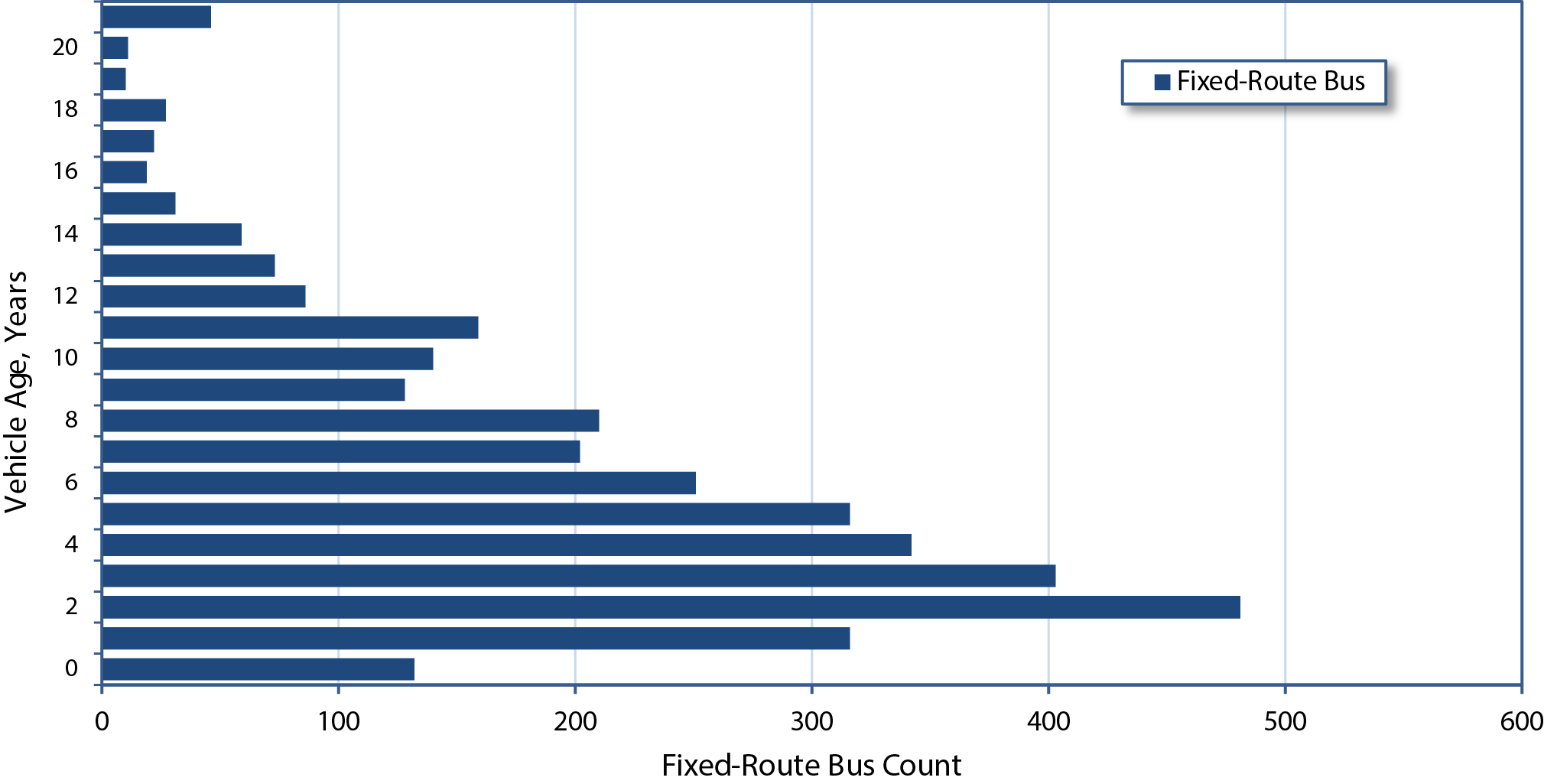
Source: Transit Economic Requirements Model and National Transit Database.
Exhibit 3-35 Age Distribution of Rural Transit Vehicles for Vans, Minivans, Autos, and Cutaways, 2012
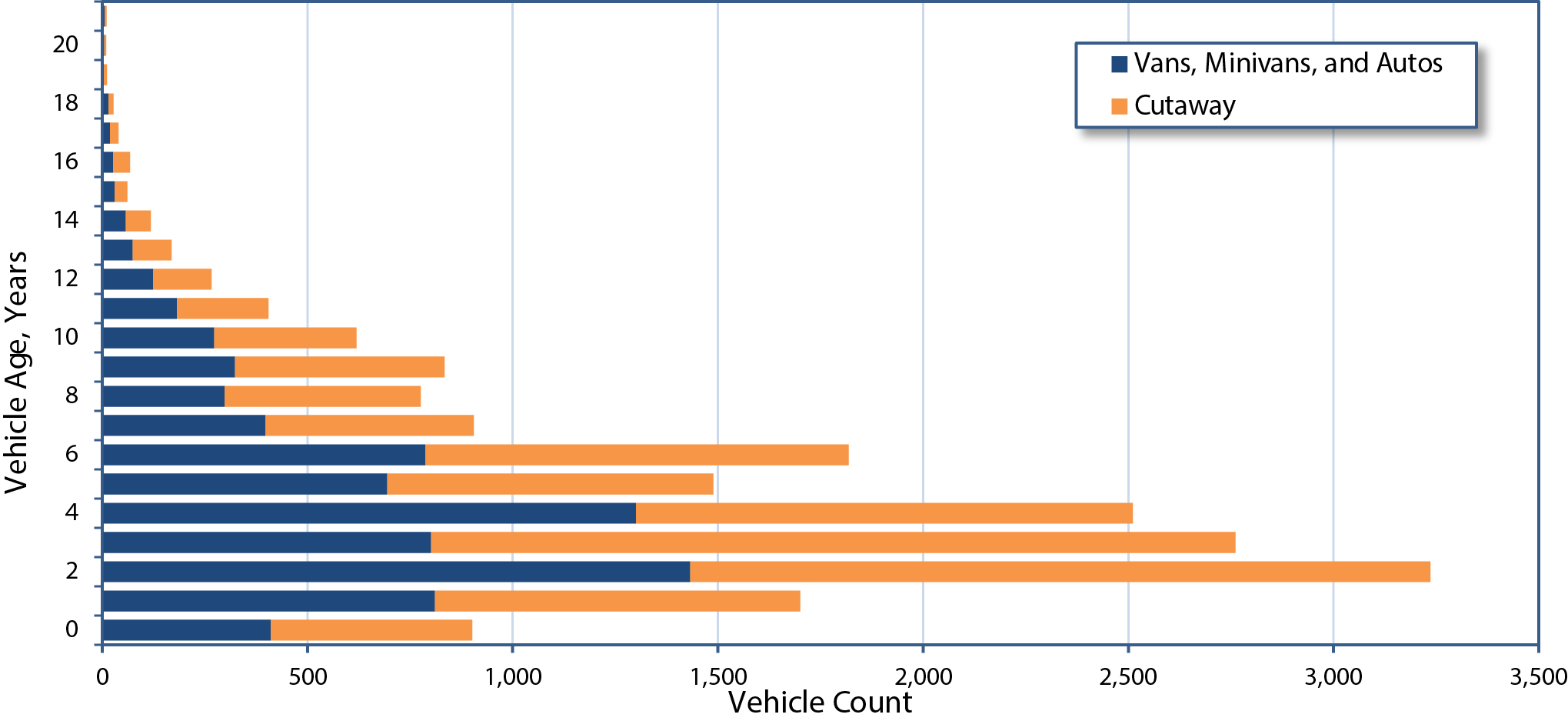
Source: Transit Economic Requirements Model and National Transit Database.
For 2012, data reported to NTD indicated that 17.0 percent of rural buses, 6.0 percent of cutaways, and 41.4 percent of rural vans were past their FTA minimum life expectancy (12 years for buses, 7 to 10 for cutaways, and 4 for vans). The rural transit fleet had an average age of 5.2 years in 2012; buses, with an average age of 8.1 years, were older than vans and cutaways, which each had an average age of 4.6 years.