U.S. Department of Transportation
Federal Highway Administration
1200 New Jersey Avenue, SE
Washington, DC 20590
202-366-4000
Description: The operational characteristic of the roadway.
Use: For determining public road mileage, for investment requirements modeling to calculate capacity and estimate roadway deficiencies and improvement needs, in the cost allocation pavement model, and in the national highway database; for the querying and analysis of data (e.g., transportation performance management (TPM) metrics, Federal-aid project information, etc.) by facility type.
Extent: All Public highways including ramps located within grade-separated interchanges as identified in 23 U.S.C 101.a(27).
Functional System |
1 |
2 |
3 |
4 |
5 |
6 |
7 |
|
|---|---|---|---|---|---|---|---|---|
NHS |
IH |
OFE |
OPA |
MiA |
MaC |
MiC |
Local |
|
Rural |
FE+R |
FE+R |
FE+R |
FE+R |
FE+R |
FE+R |
FE+R |
FE+R |
Urban |
FE+R |
FE+R |
FE+R |
FE+R |
FE+R |
FE+R |
FE+R |
FE+R |
FE + R = Full Extent & Ramps |
||||||||
Coding Requirements for Fields 8, 9, and 10:
Value_Numeric: Use one of the following codes as applicable regardless of whether or not the section is on a structure. The definition for each code is as follows:
Code |
Description |
|
|---|---|---|
1 |
One-Way Roadway |
Roadway that operates with traffic moving in a single direction during non-peak period hours. |
2 |
Two-Way Roadway |
Roadway that operates with traffic moving in both directions during non-peak period hours. |
4 |
Ramp |
Non-mainline junction or connector facility contained within a grade-separated interchange. |
5 |
Non Mainline |
All non-mainline facilities excluding ramps. |
6 |
Non Inventory Direction |
Individual road/roads of a multi-road facility that is/are not used for determining the primary length for the facility. |
7 |
Planned/Unbuilt |
Planned roadway that has yet to be constructed. |
Value_Text: No entry required. Available for State Use.
Value_Date: No entry required. Available for State Use.
Guidance: General
Public road mileage is based only on sections coded ‘1,’ or ‘2’. This includes only those roads that are open to public travel regardless of the ownership or maintenance responsibilities. Ramps are not included in the public road mileage calculation.
Frontage roads and service roads that are public roads shall be coded either as one-way (Code ‘1’) or two-way (Code ‘2’) roadways.
Use Code ‘7’ to identify a new roadway section that has been approved per the State Transportation Improvement Plan (STIP), but has yet to be built.
”One-way Pairs” (See Figure 4.5)
Characteristics:
Ramps
Ramps may consist of directional connectors from either an Interstate to another Interstate, or from an Interstate to a different functional system. Moreover, ramps allow ingress and egress to grade separated highways. Ramps may consist of traditional ramps, acceleration and deceleration lanes, as well as collector-distributor lanes.
Ramps shall be coded with the highest order functional system within the interchange that it functions. A mainline facility that terminates at the junction with another mainline facility is not a ramp and shall be coded ‘1.’
Non-Mainlines
Non-mainline facilities include roads or lanes that provide access to and from sites that are adjacent to a roadway section such as bus terminals, park and ride lots, and rest areas. These may include: special bus lanes, limited access truck roads, ramps to truck weigh stations, or a turn-around.
For LRS purposes, this Data Item shall be reported independently for both directions of travel associated with divided highway sections, for which dual carriageway GIS network representation is required per guidance in Chapter 3, Section 3.3 and Table 3.5.
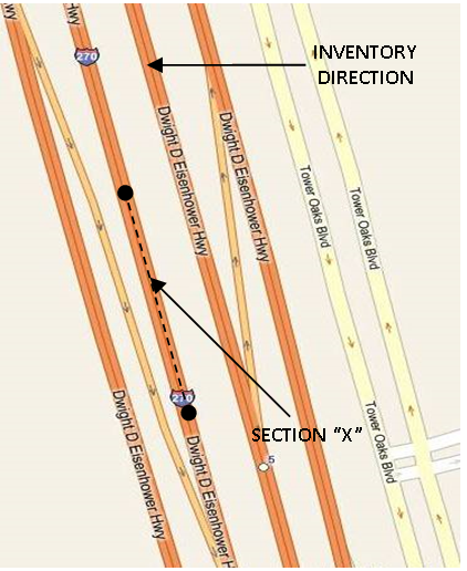
Figure 4.4 shows an example of a street (E. Baltimore St.), for which traffic is only permitted to move in the eastbound direction. In this particular case, this data item shall be assigned a Code ‘1’ for a given section (Section “X”) along this stretch of road.
Figure 4.4: One-Way Roadway (Code ‘1’) Example
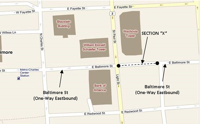
Source: Bing Maps
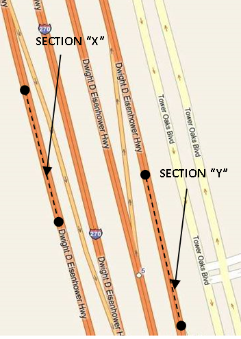
Figure 4.5 shows an example of a street (MD 198), for which traffic moves in the east and westbound directions along a set of one-way pairs (i.e., divided sections located along a given route). In this particular case, this data item shall be assigned a Code ‘1’ for section “X”, and section “Y”.
Figure 4.5: "One-Way Pairs” (Code ‘1’) Example
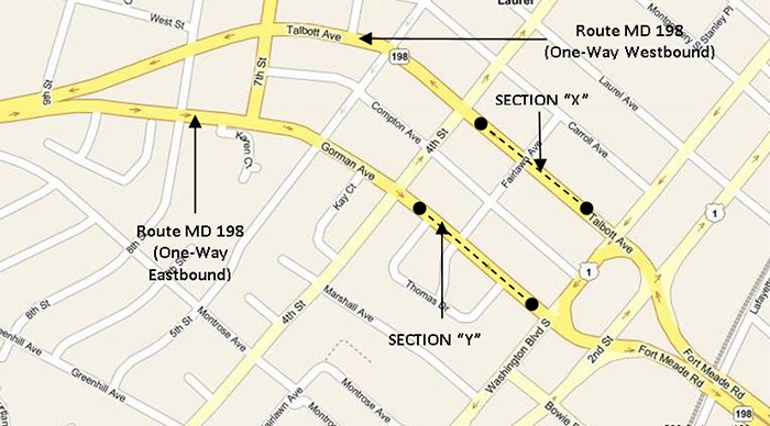
Source: Bing Maps
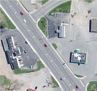
Figure 4.6 shows an example of a street (7th St. NW), for which traffic is permitted to move in both the north and southbound directions. In this particular case, this data item shall be assigned a Code ‘2’ for a given section (Section “X”) along this stretch of road.
Figure 4.6: Two-Way Roadway (Code ‘2’) Example
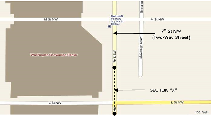
Source: Bing Maps
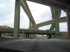
Figure 4.7 shows an example of ramps contained within a grade-separated interchange located on a highway (Interstate 495). In this particular case, this data item shall be assigned a Code ‘4’ for all applicable ramp sections (denoted as “Ramps” in the figure).
Figure 4.7: Ramp (Code ‘4’) Example
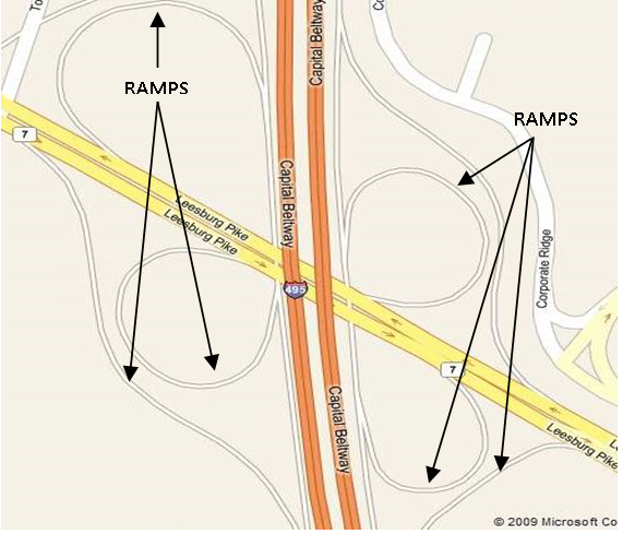
Figure 4.8 shows an example of a highway (Interstate 270), which consists of express and local lanes in both the north and southbound directions. In this particular case, this data item shall be assigned a Code ‘5’ for Sections “X” and “Y” to indicate that they are non-mainline facilities.
Figure 4.8: Non-Mainline (Code ‘5’) Example
Source: Bing Maps
Figure 4.9 shows an example of a highway (Interstate 270), for which an inventory direction is defined (northbound). In this particular case, this data item shall be assigned a Code ‘6’ for Section “X”, as the southbound side of the roadway would be defined as the non-inventory direction.
Figure 4.9: Non-Inventory Direction (Code ‘6’) Example
Source: Bing Maps
Description: Roadway section that is a bridge, tunnel or causeway.
Use: For analysis in the national highway database and pavement performance analysis/reporting
Extent: All Federal-aid highways.
Functional System |
1 |
2 |
3 |
4 |
5 |
6 |
7 |
|
|---|---|---|---|---|---|---|---|---|
NHS |
IH |
OFE |
OPA |
MiA |
MaC |
MiC |
Local |
|
Rural |
FE** |
FE** |
FE** |
FE** |
FE** |
FE** |
||
Urban |
FE** |
FE** |
FE** |
FE** |
FE** |
FE** |
FE** |
|
FE** = Full Extent wherever data item is applicable |
||||||||
Coding Requirements for Fields 8, 9, and 10:
Value_Numeric: Use the following codes:
Code |
Description |
|---|---|
1 |
Section is a Bridge |
2 |
Section is a Tunnel |
3 |
Section is a Causeway |
Value_Text: No entry required. Available for State Use.
Value_Date: No entry required. Available for State Use.
Guidance: Code this data item wherever a bridge, tunnel, or causeway exists.
Bridges shall meet a minimum length requirement of more than 20 feet (per the National Bridge Inventory (NBI) guidelines in accordance with 23 CFR 650.305) in order to be deemed a “structure.” Per NBI guidelines, bridge-sized culverts shall be reported for this data item; all other culverts are to be excluded.
A tunnel is a roadway below the surface connecting to at-grade adjacent sections.
A causeway is a narrow, low-lying raised roadway, usually providing a passageway over some type of vehicular travel impediment (e.g. a river, swamp, earth dam, wetlands, etc.).
In accordance with 23 CFR 490.309(c), this data shall be collected and reported on an annual cycle for the Interstate roadways and on a 2-year maximum cycle for all other required sections.
The begin and end points for this data item shall be coded in accordance with the points of origin and terminus for the associated bridge, tunnel or causeway. Furthermore, the points of origin and terminus for structures shall exclude approach slabs.
For LRS purposes, this Data Item can be reported independently for both directions of travel associated with divided highway sections, for which dual carriageway GIS network representation is required per guidance in Chapter 3, Section 3.3 and Table 3.5. NOTE: This data item is required to be reported for both the inventory and non-inventory directional approaches associated with all divided Interstate roadway sections where the following pavement data items have been reported in the same manner (as specified in the Metadata; see Chapter 3, Sec. 3.3, Tables 3.18 and 3.19):
Figure 4.10: Bridge (Code ‘1’) Example

Source: PennDOT
Figure 4.11: Tunnel (Code ‘2’) Example

Source: PennDOT
Figure 4.12: Causeway (Code ‘3’) Example
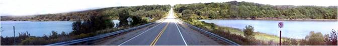
Source: PennDOT Video-log.
Description: The degree of access control for a given section of road.
Use: For investment requirements modeling to calculate capacity and estimate type of design, in truck size and weight studies, and for national highway database purposes.
Extent: All principal arterials and Sample Panel sections; optional for other non-principal arterial sections beyond the limits of the Sample Panel.
Functional System |
1 |
2 |
3 |
4 |
5 |
6 |
7 |
|
|---|---|---|---|---|---|---|---|---|
NHS |
IH |
OFE |
OPA |
MiA |
MaC |
MiC |
Local |
|
Rural |
FE |
FE |
FE |
FE |
SP |
SP |
||
Urban |
FE |
FE |
FE |
FE |
SP |
SP |
SP |
|
FE = Full Extent SP = Sample Panel Sections |
||||||||
Coding Requirements for Fields 8, 9, and 10:
Value_Numeric: Use the following codes:
Code |
Description |
|
|---|---|---|
1 |
Full Access Control |
Preference given to through traffic movements by providing interchanges with selected public roads, and by prohibiting crossing at-grade and direct driveway connections (i.e., limited access to the facility). |
2 |
Partial Access Control |
Preference given to through traffic movement. In addition to interchanges, there may be some crossings at-grade with public roads, but, direct private driveway connections have been minimized through the use of frontage roads or other local access restrictions. Control of curb cuts is not access control. |
3 |
No Access Control |
No degree of access control exists (i.e., full access to the facility is permitted). |
Value_Text: No entry required. Available for State Use.
Value_Date: No entry required. Available for State Use.
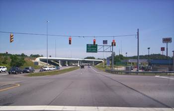
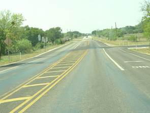
Figure 4.13: Full Control (Code ‘1’); all access via grade-separated interchanges
Source: TxDOT, Transportation Planning and Programming Division.
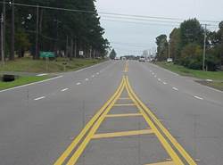
Figure 4.14: Partial Control (Code ‘2’); access via grade-separated interchanges and direct access roadways
Source: https://upload.wikimedia.org/wikipedia/commons/a/a9/Ohio_13_and_Possum_Run_Road.JPG
Figures 4.15 and 16: No Access Control (Code ‘3’)
Figure 4.15 Figure 4.16
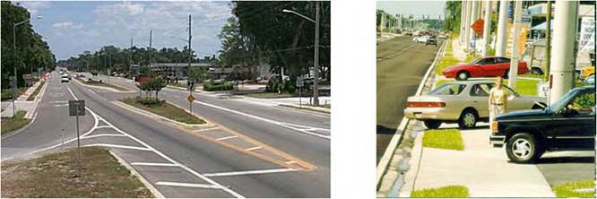
Source for Figures 4.15 and 4.16: FDOT RCI Field Handbook, Nov. 2008.
Description: The entity that has legal ownership of a roadway.
Use: For apportionment, administrative, legislative, analytical, and national highway database purposes, and in cost allocation studies; for the querying and analysis of data (e.g., transportation performance management (TPM) metrics, Federal-aid project information, etc.) by ownership.
Extent: All Public highways as identified in 23 U.S.C 101.a(27).
Functional System |
1 |
2 |
3 |
4 |
5 |
6 |
7 |
|
|---|---|---|---|---|---|---|---|---|
NHS |
IH |
OFE |
OPA |
MiA |
MaC |
MiC |
Local |
|
Rural |
FE |
FE |
FE |
FE |
FE |
FE |
FE |
FE |
Urban |
FE |
FE |
FE |
FE |
FE |
FE |
FE |
FE |
FE = Full Extent SP = Sample Panel Sections |
||||||||
Coding Requirements for Fields 8, 9, and 10:
Value_Numeric: Code the level of government that best represents the highway owner irrespective of whether agreements exist for maintenance or other purposes. If more than one code applies, code the lowest numerical value using the following codes:
Code |
Description |
Code |
Description |
|---|---|---|---|
1 |
State Highway Agency |
60 |
Other Federal Agency |
2 |
County Highway Agency |
62 |
Bureau of Indian Affairs |
3 |
Town or Township Highway Agency |
63 |
Bureau of Fish and Wildlife |
4 |
City or Municipal Highway Agency |
64 |
U.S. Forest Service |
11 |
State Park, Forest, or Reservation Agency |
66 |
National Park Service |
12 |
Local Park, Forest or Reservation Agency |
67 |
Tennessee Valley Authority |
21 |
Other State Agency |
68 |
Bureau of Land Management |
25 |
Other Local Agency |
69 |
Bureau of Reclamation |
26 |
Private (other than Railroad) |
70 |
Corps of Engineers |
27 |
Railroad |
72 |
Air Force |
31 |
State Toll Road |
73 |
Navy/Marines |
32 |
Local Toll Authority |
74 |
Army |
40 |
Other Public Instrumentality (i.e., Airport) |
80 |
Other |
50 |
Indian Tribe Nation |
Value_Text: Optional. Code secondary ownership information, if applicable.
Value_Date: No entry required. Available for State Use.
Guidance: “State” means owned by one of the 50 States, the District of Columbia, or the Commonwealth of Puerto Rico including quasi-official State commissions or organizations;
“County, local, municipal, town, or township” means owned by one of the officially recognized governments established under State authority;
“Federal” means owned by one of the branches of the U.S. Government or independent establishments, government corporations, quasi-official agencies, organizations, or instrumentalities;
“Other” means any other group not already described above or nongovernmental organizations with the authority to build, operate, or maintain toll or free highway facilities.
Only private roads that are open to public travel (e.g., toll bridges) are to be reported in HPMS.
In cases where ownership responsibilities are shared between multiple entities, this item shall be coded based on the primary owner (i.e., the entity that has the larger degree of ownership), if applicable. Information on additional owners shall be entered in Data Field 9 for this item.
For LRS purposes, this Data Item shall be reported independently for both directions of travel associated with divided highway sections, for which dual carriageway GIS network representation is required per guidance in Chapter 3, Section 3.3 and Table 3.5.
Description The number of lanes designated for through-traffic.
Use: For apportionment, administrative, legislative, analytical, pavement performance analysis/reporting and national highway database purposes.
Extent: All Federal-aid highways including ramps located within grade-separated interchanges.
Functional System |
1 |
2 |
3 |
4 |
5 |
6 |
7 |
|
|---|---|---|---|---|---|---|---|---|
NHS |
IH |
OFE |
OPA |
MiA |
MaC |
MiC |
Local |
|
Rural |
FE+R |
FE+R |
FE+R |
FE+R |
FE+R |
FE+R |
||
Urban |
FE+R |
FE+R |
FE+R |
FE+R |
FE+R |
FE+R |
FE+R |
|
FE = Full Extent & Ramps |
||||||||
Coding Requirements for Fields 8, 9, and 10:
Value_Numeric: Enter the number of through lanes in both directions carrying through traffic in the off-peak period.
Value_Text: No entry required. Available for State Use.
Value_Date: No entry required. Available for State Use.
Guidance: This Data Item shall also be reported for all ramp sections contained within grade separated interchanges.
Code the number of through lanes according to the striping, if present, on multilane facilities, or according to traffic use or State/local design guidelines if no striping or only centerline striping is present.
For one-way roadways, two-way roadways, and couplets, exclude all ramps and sections defined as auxiliary lanes, such as:
When coding the number of through lanes for ramps (i.e., where Data Item 3 = Code ‘4’), include the predominant number of (through) lanes on the ramp. Do not include turn lanes (exclusive or combined) at the termini unless they are continuous (turn) lanes over the entire length of the ramp.
Managed lanes (e.g., High Occupancy Vehicle (HOV), High Occupancy Toll (HOT), Express Toll Lanes (ETL)) operating during the off-peak period are to be included in the total count of through lanes.
This data shall be collected and reported on an annual cycle for all required sections.
For LRS purposes, this Data Item can be reported independently for both directions of travel associated with divided highway sections, for which dual carriageway GIS network representation is required per guidance in Chapter 3, Section 3.3 and Table 3.5.
Figure 4.17: A Roadway with Four Through-Lanes
Source: TxDOT, Transportation Planning and Programming Division.
Description: The type of managed lane operations (e.g., HOV, HOT, ETL, etc.).
Use: For administrative, legislative, analytical, and national highway database purposes.
Extent: All sections where managed lane operations exist. This shall correspond with the information reported for Data Item 9 (Managed Lanes).
Functional System |
1 |
2 |
3 |
4 |
5 |
6 |
7 |
|
|---|---|---|---|---|---|---|---|---|
NHS |
IH |
OFE |
OPA |
MiA |
MaC |
MiC |
Local |
|
Rural |
FE** |
FE** |
FE** |
FE** |
FE** |
FE** |
||
Urban |
FE** |
FE** |
FE** |
FE** |
FE** |
FE** |
FE** |
|
FE** = Full Extent wherever data item is applicable |
||||||||
Coding Requirements for Fields 8, 9, and 10:
Value_Numeric: Use the following codes:
Code |
Description |
|
|---|---|---|
1 |
Full-time Managed Lanes |
Section has 24-hour exclusive managed lanes (e.g., HOV use only; no other use permitted). |
2 |
Part-time Managed Lanes |
Normal through lanes used for exclusive managed lanes during specified time periods. |
3 |
Part-time Managed Lanes |
Shoulder/Parking lanes used for exclusive managed lanes during specified time periods. |
Value_Text: No Entry Required. Available for State Use.
Value_Date: No Entry Required. Available for State Use.
Guidance: Code this data item only when managed lane operations exist.
Code this Data Item for both directions to reflect existing managed lane operations. If more than one type of managed lane is present for the section, code the lesser of the two applicable Managed Lane Type codes (e.g., if Codes ‘2’ and ‘3’ are applicable for a section, then the section shall be coded as a Code ‘2’).
Alternatively, if more than one type of managed lane operation exists, the secondary Managed Lane Type may be indicated in the Value_Text field.
This information may be indicated by either managed lane signing (e.g., the presence of a large diamond-shaped marking (HOV symbol) on the pavement, or both).
Figure 4.18: HOV Signage
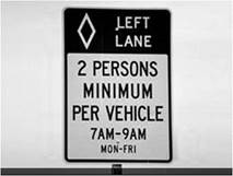
Source: FDOT RCI Field Handbook, Nov. 2008.
Item 9: HOV_Lanes (Managed Lanes)
Description: Maximum number of lanes in both directions designated for managed lane operations.
Use: For administrative, legislative, analytical, and national highway database purposes.
Extent: All Sections where managed lanes exist. This should correspond with the information reported for Data Item 8 (Managed Lane Operations Type).
Functional System |
1 |
2 |
3 |
4 |
5 |
6 |
7 |
|
|---|---|---|---|---|---|---|---|---|
NHS |
IH |
OFE |
OPA |
MiA |
MaC |
MiC |
Local |
|
Rural |
FE** |
FE** |
FE** |
FE** |
FE** |
FE** |
||
Urban |
FE** |
FE** |
FE** |
FE** |
FE** |
FE** |
FE** |
|
FE** = Full Extent wherever data item is applicable |
||||||||
Coding Requirements for Fields 8, 9, and 10:
Value_Numeric: Enter the number of managed lanes in both directions.
Value_Text: No entry required. Available for State Use.
Value_Date: No entry required. Available for State Use.
Guidance: Code this data item when Data Item 8 (Managed Lane Operations Type) is coded.
If more than one type of managed lane operation exists on the section, code this data item with respect to all managed lanes available, and indicate (in the Value_Text field) how many lanes apply to the Managed Lane Operations Type reported in Data Item 8.
Description: The number of lanes in the peak direction of flow during the peak period.
Use: For investment requirements modeling to calculate capacity, and in congestion analyses, including estimates of delay. Also used in the Highway Capacity Manual (HCM)-based capacity calculation procedure.
Extent: All Sample Panel sections, optional for all other sections beyond the limits of the Sample Panel.
Functional System |
1 |
2 |
3 |
4 |
5 |
6 |
7 |
|
|---|---|---|---|---|---|---|---|---|
NHS |
IH |
OFE |
OPA |
MiA |
MaC |
MiC |
Local |
|
Rural |
SP |
SP |
SP |
SP |
SP |
SP |
||
Urban |
SP |
SP |
SP |
SP |
SP |
SP |
SP |
|
FE = Full Extent SP = Sample Panel Sections |
||||||||
Coding Requirements for Fields 8, 9, and 10:
Value_Numeric: Code the number of through lanes used during the peak period in the peak direction.
Value_Text: No entry required. Available for State Use.
Value_Date: No entry required. Available for State Use.
Guidance: Include reversible lanes, parking lanes, or shoulders that are legally used for through-traffic for both non-HOV and HOV operation.
The peak period is represented by the period of the day when observed traffic volumes are the highest.
Figure 4.19: Peak Lanes Example (Peak Lanes = 3)
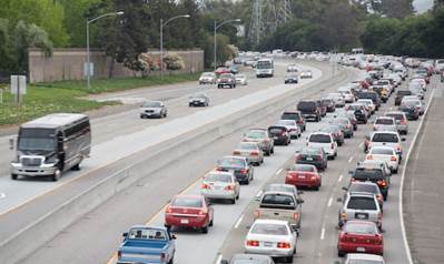
Source: Mike Kahn/Green Stock Media
Description: The number of lanes in the counter-peak direction of flow during the peak period.
Use: For investment requirements modeling to calculate capacity, and in congestion analyses, including estimates of delay. It is used in the Highway Capacity Manual (HCM)-based capacity calculation procedure.
Extent: All Sample Panel sections, optional for all other sections beyond the limits of the Sample Panel.
Functional System |
1 |
2 |
3 |
4 |
5 |
6 |
7 |
|
NHS |
IH |
OFE |
OPA |
MiA |
MaC |
MiC |
Local |
|
Rural |
SP |
SP |
SP |
SP |
SP |
SP |
||
|---|---|---|---|---|---|---|---|---|
Urban |
SP |
SP |
SP |
SP |
SP |
SP |
SP |
|
SP = Sample Panel Sections |
||||||||
Coding Requirements for Fields 8, 9, and 10:
Value_Numeric: Code the number of through lanes used during the peak period (per Data Item 10) in the counter-peak direction of flow.
Value_Text: No entry required. Available for State Use.
Value_Date: No entry required. Available for State Use.
Guidance: Include reversible lanes, parking lanes, or shoulders that are legally used for through-traffic for both non-HOV and HOV operation.
Visual inspection should be used as the principle method used to determine the number of peak lanes and counter-peak lanes.
The number of peak and counter-peak lanes should be greater than or equal to the total number of through lanes (i.e., Peak Lanes + Counter-Peak Lanes >= Through Lanes). The number of peak and counter-peak lanes can be greater than the number of through lanes if shoulders, parking lanes, or other peak-period-only lanes are used during the peak period.
The peak period is represented by the period of the day when observed traffic volumes are the highest.
Item 12: Turn_Lanes_R (Right Turn Lanes)
Description: The presence of right turn lanes at a typical intersection.
Use: For investment requirements modeling to calculate capacity and in congestion analyses, including estimates of delay.
Extent: All Sample Panel sections located in urban areas, optional for all other urban sections beyond the limits of the Sample Panel.
Functional System |
1 |
2 |
3 |
4 |
5 |
6 |
7 |
|
|---|---|---|---|---|---|---|---|---|
NHS |
IH |
OFE |
OPA |
MiA |
MaC |
MiC |
Local |
|
Rural |
||||||||
Urban |
SP |
SP |
SP |
SP |
SP |
SP |
SP |
|
SP = Sample Panel Sections |
||||||||
Coding Requirements for Fields 8, 9, and 10:
Value_Numeric: Enter the code from the following table that best describes the peak-period turning lane operation in the inventory direction.
Code |
Description |
|---|---|
1 |
No intersection where a right turning movement is permitted exists on the section. |
2 |
Turns permitted; multiple exclusive right turning lanes exist. Through movements are prohibited in these lanes. Multiple turning lanes allow for simultaneous turns from all turning lanes. |
3 |
Turns permitted; a continuous exclusive right turning lane exists from intersection to intersection. Through movements are prohibited in this lane. |
4 |
Turns permitted; a single exclusive right turning lane exists. |
5 |
Turns permitted; no exclusive right turning lanes exist. |
6 |
No right turns are permitted during the peak period. |
Value_Text: No entry required. Available for State Use.
Value_Date: No entry required. Available for State Use.
Guidance: Include turning lanes that are located at entrances to shopping centers, industrial parks, and other large traffic generating enterprises as well as public cross streets.
Where peak capacity for a section is governed by a particular intersection that is on the section, code the turning lane operation at that location (referred to as most controlling intersection); otherwise code for a typical intersection.
Through movements are prohibited in exclusive turn lanes.
Use codes ‘2’ through ‘6’ for turn lanes at a signalized or stop sign intersection that is critical to the flow of traffic; otherwise enter the code that best describes the peak-hour turning lane situation for typical intersections on the sample.
Code a continuous turning lane with painted turn bays as a continuous turning lane. Code a through lane that becomes an exclusive turning lane at an intersection as a shared (through/right turn) lane; however, if through and turning movements can be made from a lane at an intersection, it is not an exclusive turning lane.
Roundabouts (as shown in Figure 4.20) should be considered as an intersection where turns are permitted with no exclusive lanes. Use a Code ‘5’ for this item since traffic can either turn or go through the roundabout from the same lane. However, if an exclusive turning lane exists (as indicated by pavement markings), use a Code ‘4’. Code if the roundabout controls the capacity of the entire HPMS section. If there is not a controlling intersection, then code for a typical intersection.
Figure 4.20: Roundabout Configuration Example
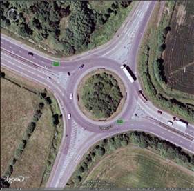
Source: SRA Consulting Group, Nov. 2008
This Data Item shall be coded based on the same intersection that is used for identifying the percent green time for a given roadway section.
Painted islands (Figure 4.21) located in the center of a roadway should be considered a median, for the purpose of determining whether or not a turn lane exists.
Slip-ramp movements should not be considered for the purpose of determining turn lanes.
On-ramps and off-ramps which provide access to and from grade-separated, intersecting roadways are to be excluded from turn lane consideration.
Figure 4.21: Painted Island Example
Source: TxDOT, Transportation Planning and Programming Division.
Figure 4.22: Multiple Turn Lanes (Code ‘2’) Example
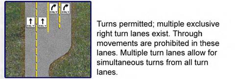
Source: FDOT RCI Field Handbook, Nov. 2008.
Figure 4.23: Continuous Turn Lane (Code ‘3’) Example
Source: Minnesota Dept. of Transportation (MnDOT).
Figure 4.24: Single Turn Lane (Code ‘4’) Example
Source: MoveTransport.com
Figure 4.25: No Exclusive Turn Lane (Code ‘5’) Example
Source: FDOT RCI Field Handbook, Nov. 2008.
Figure 4.26 No Right Turn Permitted (Code ‘6’) Example
Source: TxDOT, Transportation Planning and Programming Division.
Description: The presence of left turn lanes at a typical intersection.
Use: For investment requirements modeling to calculate capacity and in congestion analyses, including estimates of delay.
Extent: All Sample Panel sections located in urban areas, optional for all other urban sections beyond the limits of the Sample Panel.
Functional System |
1 |
2 |
3 |
4 |
5 |
6 |
7 |
|
|---|---|---|---|---|---|---|---|---|
NHS |
IH |
OFE |
OPA |
MiA |
MaC |
MiC |
Local |
|
Rural |
||||||||
Urban |
SP |
SP |
SP |
SP |
SP |
SP |
SP |
|
SP = Sample Panel Sections |
||||||||
Coding Requirements for Fields 8, 9, and 10:
Value_Numeric: Enter the code from the following table that best describes the peak-period turning lane operation in the inventory direction.
Code |
Description |
|---|---|
1 |
No intersection where a left turning movement is permitted exists on the section. |
2 |
Turns permitted; multiple exclusive left turning lanes exist. Through movements are prohibited in these lanes. Multiple turning lanes allow for simultaneous turns from all turning lanes. |
3 |
Turns permitted; a continuous exclusive left turning lane exists from intersection to intersection. Through movements are prohibited in this lane. |
4 |
Turns permitted; a single exclusive left turning lane exists. |
5 |
Turns permitted; no exclusive left turning lanes exist. |
6 |
No left turns are permitted during the peak period. |
Value_Text: No entry required. Available for State Use.
Value_Date: No entry required. Available for State Use.
Guidance: Where peak capacity for a section is governed by a particular intersection that is on the section, code the turning lane operation at that location (referred to as most controlling intersection); otherwise code for a typical intersection.
Include turning lanes that are located at entrances to shopping centers, industrial parks, and other large traffic generating enterprises as well as public cross streets.
Through movements are prohibited in exclusive turn lanes.
Use codes ‘2’ through ‘6’ for turn lanes at a signalized or stop sign intersection that is critical to the flow of traffic; otherwise enter the code that best describes the peak-hour turning lane situation for typical intersections on the sample.
Code a continuous turning lane with painted turn bays as a continuous turning lane. Code a through lane that becomes an exclusive turning lane at an intersection as a shared (through/left turn) lane; however, if through and turning movements can be made from a lane at an intersection, it is not an exclusive turning lane.
Roundabouts (as shown in Figure 4.20) should be considered as an intersection where turns are permitted with no exclusive lanes. Use a Code ‘5’ for this item since traffic can either turn or go through the roundabout from the same lane. Code if the roundabout controls the capacity of the entire HPMS section. If there is not a controlling intersection, then code for a typical intersection.
On-ramps and off-ramps which provide access to and from grade-separated, intersecting roadways are to be excluded from turn lane consideration.
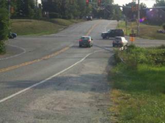
Figure 4.27: Jug Handle Configuration Example
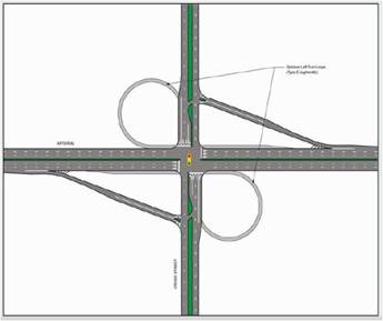
Source: SRA Consulting Group, Nov. 2008
Jug handle configurations (as shown in Figure 4.27), or lanes on either side of the roadway should be considered as an intersection with protected (exclusive) left turn lanes. Although a jug handle may be viewed as a right turn lane, it is intended for left turn movements, therefore it should not be coded as a right turn lane; instead use Code ‘6.’
This Data Item shall be coded based on the same intersection that is used for identifying the percent green time for a given roadway section.
Painted islands located in the center of a roadway should be considered a median, for the purposes of determining whether or not a turn lane exists.
Permitted U-turn movements are not to be considered for the purpose of determining turn lanes.
Figure 4.28: Multiple Turn Lanes (Code ‘2’) Example
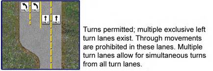
Source: FDOT RCI Field Handbook, Nov. 2008.
Figure 4.29: Multiple Turn Lanes (Code ‘2’) Example
Source: Unavailable
Figure 4.30: Continuous Turn Lane (Code ‘3’) Example
Source: Kentucky Transportation Cabinet
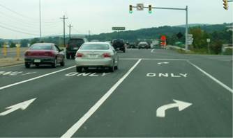
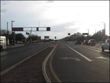
For an intersection that has a single left turn lane and no right turn lane with turns permitted in the peak period (as shown in Figure 4.31), use a code ‘4’ for this Data Item, and a code ‘5’ (turns permitted; no exclusive right turning lane exists) for Data Item 12 (Right Turn Lanes). Additionally, this intersection has four through-lanes (Data Item 7), and two peak-lanes (Data Item 10).
Figure 4.31: Exclusive Turn Lane (Code ‘4’) Example

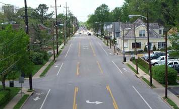
Figure 4.32: No Exclusive Left Turn Lane (Code ‘5’) Example
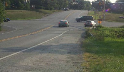
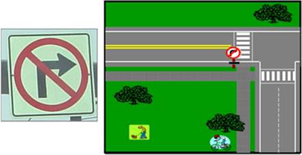
Figure 4.33: No Left Turn Permitted (Code ‘6’)

Description: The posted speed limit.
Use: For investment requirements modeling to estimate running speed and for other analysis purposes, including delay estimation.
Extent: All Sample Panel sections, optional for all other sections beyond the limits of the Sample Panel.
Functional System |
1 |
2 |
3 |
4 |
5 |
6 |
7 |
|
|---|---|---|---|---|---|---|---|---|
NHS |
IH |
OFE |
OPA |
MiA |
MaC |
MiC |
Local |
|
Rural |
FE |
FE |
SP |
SP |
SP |
SP |
||
Urban |
FE |
FE |
SP |
SP |
SP |
SP |
SP |
|
SP = Sample Panel Sections |
||||||||
Coding Requirements for Fields 8, 9, and 10:
Value_Numeric: Enter the daytime speed limit for automobiles posted or legally mandated on the greater part of the section. If there is no legally mandated maximum daytime speed limit for automobiles, code ‘999’.
Value_Text: No entry required. Available for State Use.
Value_Date: No entry required. Available for State Use.
Guidance: If the speed limit changes within the limits of a section, the State shall determine and report the predominant speed limit.
Baseline speed limit data for the National Highway System (NHS) will be provided by FHWA. The State shall validate or update this information annually as needed.
Description: Identifies sections that are toll facilities regardless of whether or not a toll is charged.
Use: For administrative, legislative, analytical, and national highway database purposes.
Extent: All roadways that are toll facilities, whether public or privately-owned / operated.
Functional System |
1 |
2 |
3 |
4 |
5 |
6 |
7 |
|
|---|---|---|---|---|---|---|---|---|
NHS |
IH |
OFE |
OPA |
MiA |
MaC |
MiC |
Local |
|
Rural |
FE** |
FE** |
FE** |
FE** |
FE** |
FE** |
FE** |
FE** |
Urban |
FE** |
FE** |
FE** |
FE** |
FE** |
FE** |
FE** |
FE** |
FE** = Full Extent wherever data item is applicable |
||||||||
Coding Requirements for Fields 8, 9, and 10:
Value_Numeric: Use the following codes:
Code |
Description |
|---|---|
1 |
Toll charged in one direction only. |
2 |
Toll charged in both directions. |
3 |
No toll charged |
Value_Text: Assign the appropriate Toll ID. See Appendix D for the list of IDs.
Value_Date: No entry required. Available for State Use.
Guidance: Code this data item only when a toll facility is present.
Code each toll and non-toll portion of contiguous toll facilities as separate sections.
If tolls are charged in both directions, but only one direction at a given time, then use Code ‘1’.
Include High Occupancy Toll (HOT) lanes and other special toll lanes. Use Code ‘3’ for subsections of a toll facility that do not have tolls.
Figure 4.34: Toll-Road Signage
Source: FDOT RCI Field Handbook, Nov. 2008.
Description: Indicates the presence of special tolls (i.e., High Occupancy Toll (HOT) lane(s) or other managed lanes).
Use: For administrative, legislative, analytical, and national highway database purposes.
Extent: All roadways where special tolls exist.
Functional System |
1 |
2 |
3 |
4 |
5 |
6 |
7 |
|
|---|---|---|---|---|---|---|---|---|
NHS |
IH |
OFE |
OPA |
MiA |
MaC |
MiC |
Local |
|
Rural |
FE** |
FE** |
FE** |
FE** |
FE** |
FE** |
FE** |
FE** |
Urban |
FE** |
FE** |
FE** |
FE** |
FE** |
FE** |
FE** |
FE** |
FE** = Full Extent wherever data item is applicable 7 |
||||||||
Coding Requirements for Fields 8, 9, and 10:
Value_Numeric: Use the following codes:
Code |
Description |
|---|---|
1 |
This section has toll lanes but no special tolls (e.g., HOT lanes). |
2 |
This section has HOT lanes. |
3 |
This section has other special tolls. |
Value_Text: Assign the appropriate Toll ID. See Appendix D for the list of IDs.
Value_Date: No entry required. Available for State Use.
Guidance: This may not be an HOV facility, but has special lanes identified where users would be subject to tolls.
High Occupancy Toll (HOT) lanes are HOV lanes where a fee is charged, sometimes based on occupancy of the vehicle or the type of vehicle. Vehicle types may include buses, vans, or other passenger vehicles.
Item 17: Route_Number (Route Number)
Description: The signed route number.
Use: Used along with route signing and route qualifier to track information by specific route.
Extent: All principal arterials, minor arterials, and the entire NHS.
Functional System |
1 |
2 |
3 |
4 |
5 |
6 |
7 |
|
|---|---|---|---|---|---|---|---|---|
NHS |
IH |
OFE |
OPA |
MiA |
MaC |
MiC |
Local |
|
Rural |
FE |
FE |
FE |
FE |
FE |
|||
Urban |
FE |
FE |
FE |
FE |
FE |
|||
FE = Full Extent |
||||||||
Coding Requirements for Fields 8, 9, and 10:
Value_Numeric: Code the appropriate route number (leading zeroes shall not be used), e.g., Interstate 81 shall be coded as ‘81’; Interstate 35W shall be coded as ‘35’.
Value_Text: Enter the full route number, e.g., “35W” or “291A.”
Value_Date: No entry required. Available for State Use.
Guidance: This shall be the same route number that is identified for the route in Data Items 18 and 19 (Route Signing and Route Qualifier).
If two or more routes of the same functional system are signed along a roadway section (e.g., Interstate 64 and Interstate 81), code the lowest route number (i.e., Interstate 64).
If two or more routes of differing functional systems are signed along a roadway section (e.g., Interstate 83 and U.S. 32), code this Data Item in accordance with the highest functional system on the route (in this example, Interstate).
For the official Interstate route number, enter an alphanumeric value for the route in Data Field 9.
If Data Items 18 or 19 (Route Signing or Route Qualifier) are coded ‘10,’ code a text descriptor (in Field 9) for this Data Item.
If the official route number contains an alphabetic character (e.g. “32A”), then code the numeric portion of this value in Field 8, and the entire value in Field 9.
Where a route is designated with alphabetic characters only (e.g. “W”), then don’t code the Value_Numeric field for this item and use the Value_Text field for the route name.
For LRS purposes, this Data Item can be reported independently for both directions of travel associated with divided highway sections, for which dual carriageway GIS network representation is required per guidance in Chapter 3, Section 3.3 and Table 3.5. NOTE: This data item is required to be reported for both the inventory and non-inventory directional approaches associated with all divided Interstate roadway sections where the following pavement data items have been reported in the same manner (as specified in the Metadata; see Chapter 3, Sec. 3.3, Tables 3.18 and 3.19):
Description: The type of route signing.
Use: For tracking information by specific route; used in conjunction with Data Item 19 (Route Qualifier).
Extent: All principal arterials, minor arterials, and the entire NHS.
Functional System |
1 |
2 |
3 |
4 |
5 |
6 |
7 |
|
|---|---|---|---|---|---|---|---|---|
NHS |
IH |
OFE |
OPA |
MiA |
MaC |
MiC |
Local |
|
Rural |
FE |
FE |
FE |
FE |
FE |
|||
Urban |
FE |
FE |
FE |
FE |
FE |
|||
FE = Full Extent |
||||||||
Coding Requirements for Fields 8, 9, and 10:
Value_Numeric: Code the value that best represents the manner in which the roadway section is signed with route markers, using the following codes:
Code |
Description |
Code |
Description |
1 |
Not Signed |
6 |
County |
2 |
Interstate |
7 |
Township |
3 |
U.S. |
8 |
Municipal |
4 |
State |
9 |
Parkway Marker or Forest Route Marker |
5 |
Off-Interstate Business Marker |
10 |
None of the Above |
Value_Text: No entry required. Available for State Use.
Value_Date: No entry required. Available for State Use.
Guidance: When a section is signed with two or more identifiers (e.g., Interstate 83 and U.S. 32), code the highest order identifier on the route (in this example, Interstate). Follow the hierarchy as ordered above.
Description: The route signing descriptive qualifier.
Use: For tracking information by specific route; used in conjunction with Data Item 18 (Route Signing).
Extent: All principal arterials, minor arterials, and the entire NHS.
Functional System |
1 |
2 |
3 |
4 |
5 |
6 |
7 |
|
|---|---|---|---|---|---|---|---|---|
NHS |
IH |
OFE |
OPA |
MiA |
MaC |
MiC |
Local |
|
Rural |
FE |
FE |
FE |
FE |
FE |
|||
Urban |
FE |
FE |
FE |
FE |
FE |
|||
FE = Full Extent |
||||||||
Coding Requirements for Fields 8, 9, and 10:
Value_Numeric: Code the value which best represents the manner in which the roadway section is signed on the route marker described in Data Item 18 (Route Signing).
Code |
Description |
Code |
Description |
|---|---|---|---|
1 |
No qualifier or Not Signed |
6 |
Loop |
2 |
Alternate |
7 |
Proposed |
3 |
Business Route |
8 |
Temporary |
4 |
Bypass Business |
9 |
Truck Route |
5 |
Spur |
10 |
None of the Above |
Value_Text: No entry required. Available for State Use.
Value_Date: No entry required. Available for State Use.
Guidance: If more than one code is applicable, use the lowest code.
Figure 4.35 Business Route (Code ‘3’) Example

Source: FDOT RCI Field Handbook, Nov. 2008.
Figure 4.36 Proposed Route (Code ‘7’) Example
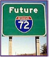
Source: FDOT RCI Field Handbook, Nov. 2008.
Figure 4.37 Temporary Route (Code ‘8’) Example

Source: FDOT RCI Field Handbook, Nov. 2008.
Description: A familiar, non-numeric designation for a route.
Use: For tracking information by specific route; used in conjunction with Data Items 18 and 19 (Route Signing and Route Qualifier).
Extent: Optional for principal arterial, minor arterial, and NHS sections where this situation exists.
Functional System |
1 |
2 |
3 |
4 |
5 |
6 |
7 |
|
|---|---|---|---|---|---|---|---|---|
NHS |
IH |
OFE |
OPA |
MiA |
MaC |
MiC |
Local |
|
Rural |
FE |
FE |
FE |
FE |
FE |
|||
Urban |
FE |
FE |
FE |
FE |
FE |
|||
FE = Full Extent |
||||||||
Coding Requirements for Fields 8, 9, and 10:
Value_Numeric: No entry required. Available for State Use.
Value_Text: Optional. Enter the alternative route name.
Value_Date: No entry required. Available for State Use.
Guidance: Examples for this Data item would be the “Pacific Coast Highway” (in California), and the “Garden State Parkway” (in New Jersey).
Description: Annual Average Daily Traffic.
Use: For apportionment, administrative, legislative, analytical, and national highway database purposes.
Extent: All Federal-aid highways including ramps located within grade-separated interchanges.
Functional System |
1 |
2 |
3 |
4 |
5 |
6 |
7 |
|
|---|---|---|---|---|---|---|---|---|
NHS |
IH |
OFE |
OPA |
MiA |
MaC |
MiC |
Local |
|
Rural |
FE+R |
FE+R |
FE+R |
FE+R |
FE+R |
FE+R |
||
Urban |
FE+R |
FE+R |
FE+R |
FE+R |
FE+R |
FE+R |
FE+R |
|
FE + R = Full Extent & Ramps |
||||||||
Coding Requirements for Fields 8, 9, and 10:
Value_Numeric: Enter a value that represents the AADT for the current data year.
Value_Text: No entry required. Available for State Use.
Value_Date: No entry required. Available for State Use.
Metadata: See Chapter 3 for a description of the metadata reporting requirements for this Data Item.
Guidance: For two-way facilities, provide the bidirectional AADT; for one-way roadways, and ramps, provide the directional AADT.
This Data Item shall also be reported for all ramp sections contained within grade separated interchanges
All AADTs shall reflect application of day of week, seasonal, and axle correction factors, as necessary; no other adjustment factors shall be used. Growth factors shall be applied if the AADT is not derived from current year counts.
AADTs for the NHS, Interstate, Principal Arterial (OFE, OPA) roadway sections shall be based on traffic counts taken on a minimum three-year cycle. AADTs for the non-Principal Arterial System (i.e., Minor Arterials, Major Collectors, and Urban Minor Collectors) can be based on a minimum six-year counting cycle.
If average weekday, average weekly, or average monthly traffic is calculated or available, it shall be adjusted to represent the annual average daily traffic (AADT). AADT is an average daily value that represents all days of the reporting year.
AADT guidance for ramps:
AADT values representing the current data year are required for ramps contained within grade separated interchanges on all Federal-aid highways. To the extent possible, the same procedures used to develop AADTs on non-ramp sections should also be used to develop AADT for data. At a minimum, 48-hour ramp traffic counts shall be taken on a six-year cycle, so at least one-sixth of the ramps should be counted every year.
Ramp AADT data may be available from freeway monitoring programs that continuously monitor travel on ramps and mainline facilities. Ramp balancing programs implemented by the States for ramp locations and on high volume roadways could be used to gather traffic data on ramps. States are encouraged to use adjustment factors that have been developed based either on entrance or exit travel patterns, or on the functional system of the ramp. The procedure should be applied consistently statewide.
Additional guidance on how this data is to be developed and reported is contained in Chapter 5.
Description: Annual Average Daily Traffic for single-unit trucks and buses.
Use: For investment requirements modeling to estimate pavement deterioration and operating speeds, in the cost allocation pavement model, the truck size and weight analysis process, freight analysis, and other scenario based analysis.
Extent: All NHS and Sample Panel sections; optional for all other non-NHS sections beyond the limits of the Sample Panel.
Functional System |
1 |
2 |
3 |
4 |
5 |
6 |
7 |
|
|---|---|---|---|---|---|---|---|---|
NHS |
IH |
OFE |
OPA |
MiA |
MaC |
MiC |
Local |
|
Rural |
FE |
FE |
SP |
SP |
SP |
SP |
||
Urban |
FE |
FE |
SP |
SP |
SP |
SP |
SP |
|
FE = Full Extent SP = Sample Panel Sections |
||||||||
Coding Requirements for Fields 8, 9, and 10:
Value_Numeric: Enter the volume for all single-unit truck and bus activity over all days of the week and seasons of the year in terms of the annual average daily traffic.
Value_Text: No entry required. Available for State Use.
Value_Date: No entry required. Available for State Use.
Metadata: See Chapter 3 for a description of the AADT metadata reporting requirements related to this Data Item.
Guidance: For two-way facilities, provide the bidirectional Single-unit Truck and Bus AADT; for one-way roadways, and ramps, provide the directional Single-unit Truck and Bus AADT.
This value shall be representative of all single-unit truck and bus activity based on vehicle classification count data from both the State’s and other agency’s traffic monitoring programs over all days of the week and all seasons of the year. Actual vehicle classification counts shall be adjusted to represent average conditions as recommended in the Traffic Monitoring Guide (TMG). Single-unit trucks and buses are defined as vehicle classes 4 through 7 (buses through four-or-more axle, single-unit trucks).
AADT values shall be updated annually to represent current year data.
Section specific measured values are requestedbased on traffic counts taken on a minimum three-year cycle. If these data are not available, values derived from classification station data on the same route, or on a similar route with similar traffic characteristics in the same area can be used.
Specific guidance for the frequency and size of vehicle classification data collection programs, factor development, age of data, and other applications is contained in the Traffic Monitoring Guide.
Description: Peak hour single-unit truck and bus volume as a percentage of total AADT.
Use: For investment requirements modeling to calculate capacity and peak volumes.
Extent: All Sample Panel sections; optional for all other sections beyond the limits of the Sample Panel.
Functional System |
1 |
2 |
3 |
4 |
5 |
6 |
7 |
|
|---|---|---|---|---|---|---|---|---|
NHS |
IH |
OFE |
OPA |
MiA |
MaC |
MiC |
Local |
|
Rural |
SP |
SP |
SP |
SP |
SP |
SP |
||
Urban |
SP |
SP |
SP |
SP |
SP |
SP |
SP |
|
SP = Sample Panel Sections |
||||||||
Coding Requirements for Fields 8, 9, and 10:
Value_Numeric: Enter the peak hour single-unit truck and bus volume as a percentage of the applicable roadway section’s AADT rounded to the nearest thousandth of a percent (0.001%). This percent shall not be rounded to the nearest whole percent or to zero percent if minimal vehicles exist.
Value_Text: No entry required. Available for State Use.
Value_Date: No entry required. Available for State Use.
Guidance: Code this itembased on vehicle classification data from traffic monitoring programs for vehicle classes 4 through 7 (as defined in the Traffic Monitoring Guide), based on traffic counts taken on a three-year cycle, at a minimum.
The Percent Peak Single-Unit Trucks and Buses value is calculated by dividing the number of single-unit trucks and buses during the hour with the highest total volume (i.e. the peak hour) by the AADT (i.e. the total daily traffic). Note that this data item is based on the truck traffic during the peak traffic hour and not the hour with the most truck traffic.
If actual measured values are not available, then an estimate shall be made based on the most readily available information. The most credible method would be to use other site specific measured values from sites located on the same route. Other methods may include: assigning site specific measured values to other samples that are located on similar facilities with similar traffic characteristics in the same geographic area and in the same volume group; or assigning measured values from samples in the same functional system and in the same area type ( i.e., rural, small urban, urbanized).
Statewide or functional system-wide values shall not be used. Peak hour values may be different than daily averages which must be taken into consideration.
Supplemental methods and sources may be particularly useful in urban areas. These include turning movement studies, origin and destination studies, license plate surveys, design estimates and projections, and MPO data obtained for other purposes. Short term visual observation of truck travel can also be helpful when developing an estimate.
Note that this data represents the truck traffic during the peak traffic hour, not the 30th highest hourly volume for a given calendar year or the hour which has the peak truck traffic (see Figure 4.38).
Figure 4.38 Peak Hour Truck Traffic vs. AADT

Code this data item in accordance with the limits for which Data Item #22 is reported.
The following examples illustrate the % Peak Single-Unit (SU) Trucks calculation:
Example #1
AADT = 150,000 vehicles
SU AADT = 12,100 SU trucks (classes 4-7)
Peak hour SU Trucks = 1,550 SU trucks (classes 4-7)
% Peak SU Trucks = (Peak hour SU trucks/AADT)*100 =
(1,550 SU trucks/150,000)*100 = 1.0333%
*When reported in HPMS, this % Peak SU value would be reported as 1.033%.
Example #2
AADT = 2,050 vehicles
SU AADT = 85 SU trucks (classes 4-7)
Peak hour SU Trucks = 8 SU trucks (classes 4-7)
% Peak SU Trucks = (Peak hour SU trucks/AADT)*100
(8 SU trucks/2,050)*100 = 0.39024%
*When reported in HPMS, this % Peak SU value would be reported as 0.390%.
Description: Annual Average Daily Traffic for Combination Trucks.
Use: For investment requirements modeling to estimate pavement deterioration and operating speeds, in the cost allocation pavement model, the truck size and weight analysis process, and freight analysis.
Extent: All NHS and Sample Panel sections; optional for all other non-NHS sections beyond the limits of the Sample Panel.
Functional System |
1 |
2 |
3 |
4 |
5 |
6 |
7 |
|
|---|---|---|---|---|---|---|---|---|
NHS |
IH |
OFE |
OPA |
MiA |
MaC |
MiC |
Local |
|
Rural |
FE |
FE |
SP |
SP |
SP |
SP |
||
Urban |
FE |
FE |
SP |
SP |
SP |
SP |
SP |
|
FE = Full Extent SP = Sample Panel Sections |
||||||||
Coding Requirements for Fields 8, 9, and 10:
Value_Numeric: Enter the volume for combination-unit truck activity over all days of the week and seasons of the year in terms of the annual average daily traffic.
Value_Text: No entry required. Available for State Use.
Value_Date: No entry required. Available for State Use.
Metadata: See Chapter 3 for a description of the AADT metadata reporting requirements related to this Data Item.
Guidance: For two-way facilities, provide the bidirectional Combination Truck AADT; for one-way roadways, and ramps, provide the directional Combination Truck AADT.
This value shall be representative of all combination truck activity based on vehicle classification data from traffic monitoring programs over all days of the week and all seasons of the year. Actual vehicle classification counts shall be adjusted to represent average conditions as recommended in the Traffic Monitoring Guide (TMG). Combination trucks are defined as vehicle classes 8 through 13 (four-or-less axle, single-trailer trucks through seven-or-more axle, multi-trailer trucks).
AADT values shall be updated annually to represent current year data.
Section specific measured values are requestedbased on traffic counts taken on a three-year cycle, at a minimum. If these data are not available, use values derived from classification station data on the same route or on a similar route with similar traffic characteristics in the same area.
Specific guidance for the frequency and size of vehicle classification data collection programs, factor development, age of data, and other applications is contained in the Traffic Monitoring Guide.
Description: Peak hour combination truck volume as a percentage of total AADT.
Use: For investment requirements modeling to calculate capacity and peak volumes.
Extent: All Sample Panel sections; optional for all other sections beyond the limits of the Sample Panel.
Functional System |
1 |
2 |
3 |
4 |
5 |
6 |
7 |
|
|---|---|---|---|---|---|---|---|---|
NHS |
IH |
OFE |
OPA |
MiA |
MaC |
MiC |
Local |
|
Rural |
SP |
SP |
SP |
SP |
SP |
SP |
||
Urban |
SP |
SP |
SP |
SP |
SP |
SP |
SP |
|
SP = Sample Panel Sections |
||||||||
Coding Requirements for Fields 8, 9, and 10:
Value_Numeric: Enter the peak hour combination truck volume as a percentage of the applicable roadway section’s AADT rounded to the nearest thousandth of a percent (0.001%). This percent shall not be rounded to the nearest whole percent or to zero percent if minimal vehicles exist.
Value_Text: No entry required. Available for State Use.
Value_Date: No entry required. Available for State Use.
Guidance: Code this item based on vehicle classification data from traffic monitoring programs for vehicle classes 8 through 13 (as defined in the TMG) based on traffic counts taken on a three year cycle, as a minimum. Code this data item in accordance with the limits for which Data Item #24 is reported.
The Percent Peak Combination Truck value is calculated by dividing the number of combination trucks during the hour with the highest total volume (i.e. the peak hour) by the AADT (i.e. the total daily traffic). Note that this data item is based on the truck traffic during the peak traffic hour and not the hour with the most truck traffic.
If actual measured values are not available, then an estimate shall be made based on the most readily available information. The most credible method would be to use other site specific measured values from sites located on the same route. Other methods may include: assigning site specific measured values to other samples that are located on similar facilities with similar traffic characteristics in the same geographic area and in the same volume group; or assigning measured values from samples in the same functional system and in the same area type ( i.e., rural, small urban, urbanized).
Statewide or functional system-wide values shall not be used. Peak hour values may be different than daily averages which must be taken into consideration.
Supplemental methods and sources may be particularly useful in urban areas. These include turning movement studies, origin and destination studies, license plate surveys, design estimates and projections, and MPO data obtained for other purposes. Short term visual observation of truck travel can also be helpful when developing an estimate.
Note that this data represents the truck traffic during the peak traffic hour, not the 30th highest hourly volume for a given calendar year or the hour which has the peak truck traffic (see Figure 4.38).
The following examples illustrate the % Peak Combination-Unit (CU) Trucks calculation:
Example #1
AADT = 15,000 vehicles
CU AADT = 2,800 CU trucks (classes 8-13)
Peak hour CU Trucks = 215 CU trucks (classes 8-13)
% Peak CU Trucks = (Peak hour CU Trucks/AADT)*100 =
(215 CU Trucks/15,000)*100 = 1.433%
*When reported in HPMS, this % Peak CU value would be reported as 1.433%.
Example #2
AADT = 70,240 vehicles
CU AADT = 22,750 CU Trucks (classes 8-13)
Peak hour CU Trucks = 1,528 CU Trucks (classes 8-13)
% Peak CU Trucks = (Peak hour CU Trucks/AADT)*100
(1,528 CU Trucks/70,240)*100 = 2.175%
*When reported in HPMS, this % Peak CU value would be reported as 2.175%.
Description: The design hour volume (30th largest hourly volume for a given calendar year) as a percentage of AADT.
Use: For investment requirements modeling to calculate capacity and estimate needed capacity improvements, in the cost allocation pavement model, and for other analysis purposes, including delay estimation.
Extent: All Sample Panel sections; optional for all other sections beyond the limits of the Sample Panel.
Functional System |
1 |
2 |
3 |
4 |
5 |
6 |
7 |
|
NHS |
IH |
OFE |
OPA |
MiA |
MaC |
MiC |
Local |
|
Rural |
SP |
SP |
SP |
SP |
SP |
SP |
||
Urban |
SP |
SP |
SP |
SP |
SP |
SP |
SP |
|
SP = Sample Panel Sections |
||||||||
Coding Requirements for Fields 8, 9, and 10:
Value_Numeric: Enter the K-factor to the nearest percent.
Value_Text: No entry required. Available for State Use.
Value_Date: No entry required. Available for State Use.
Guidance: The K-factor is the design hour volume commonly known as, the 30th largest hourly volume for a given calendar year as a percentage of the annual average daily traffic. Section specific values shall be provided. Statewide or functional system-wide values shall not be used. .
The best source of this data is from continuous traffic monitoring sites. If continuous data is not available, use values derived from continuous count station data on the same route or on a similar route with similar traffic characteristics in the same area.
When utilizing traffic count data gathered from continuous traffic monitoring sites, the 30th highest hourly volume for a given year (typically used) is to be used for the purposes of calculating K-factor.
Other sources of this data may include the use of project level information for the section, turning movement and classification count data, regression analysis of computed K-factors at continuous count stations (CCSs), continuous site data grouped by urbanized areas to estimate urbanized area K-factors, and continuous site data grouped by number of lanes for high volume routes.
The hour used to calculate K-factor should also be used to calculate D-factor.
Code this data item in accordance with the limits for which Data Item #21 is reported.
Description: The percent of design hour volume (30th largest hourly volume for a given calendar year) flowing in the higher volume direction.
Use: For investment requirements modeling to calculate capacity and estimate needed capacity improvements, in congestion, delay, and other analyses, and in the cost allocation pavement model.
Extent: All Sample Panel sections; optional for all other sections beyond the limits of the Sample Panel.
Functional System |
1 |
2 |
3 |
4 |
5 |
6 |
7 |
|
|---|---|---|---|---|---|---|---|---|
NHS |
IH |
OFE |
OPA |
MiA |
MaC |
MiC |
Local |
|
Rural |
SP |
SP |
SP |
SP |
SP |
SP |
||
Urban |
SP |
SP |
SP |
SP |
SP |
SP |
SP |
|
SP = Sample Panel Sections |
||||||||
Coding Requirements for Fields 8, 9, and 10:
Value_Numeric: Enter the percentage of the design hour volume flowing in the peak direction. Code ‘100’ for one-way facilities.
Value_Text: No entry required. Available for State Use.
Value_Date: No entry required. Available for State Use.
Guidance: Section-specific values based on an actual count shall be provided. If this information is unavailable, use values derived from continuous count station data on the same route or on a similar route with similar traffic characteristics in the same area. Statewide or functional system-wide values shall not be used.
For two-way facilities, the directional factor normally ranges from 50 to 70 percent.
When utilizing traffic count data gathered from continuous traffic monitoring sites, the 30th highest hourly volume for a given year (typically used) is to be used for the purposes of calculating D-factor.
The hour used to calculate D-factor should also be used to calculate K-factor.
Code this data item in accordance with the limits for which Data Item #21 is reported.
Description: Forecasted AADT.
Use: For investment requirements modeling to estimate deficiencies and future improvement needs, in the cost allocation pavement model and in other analytical studies.
Extent: All Sample Panel sections; optional for all other sections beyond the limits of the Sample Panel.
Functional System |
1 |
2 |
3 |
4 |
5 |
6 |
7 |
|
|---|---|---|---|---|---|---|---|---|
NHS |
IH |
OFE |
OPA |
MiA |
MaC |
MiC |
Local |
|
Rural |
SP |
SP |
SP |
SP |
SP |
SP |
||
Urban |
SP |
SP |
SP |
SP |
SP |
SP |
SP |
|
SP = Sample Panel Sections |
||||||||
Coding Requirements for Fields 8, 9, and 10:
Value_Numeric: Enter a value that represents the forecasted AADT.
Value_Text: No entry required. Available for State Use.
Value_Date: Four-digit year for which the Future AADT has been forecasted.
Guidance: For two-way facilities, provide the bidirectional Future AADT; for one-way roadways, and ramps, provide the directional Future AADT.
This should be a 20-year forecast AADT, which may cover a period of 18 to 25 year periods from the data year of the submittal, and must be updated if less than 18 years.
Future AADT should come from a technically supportable State procedure, Metropolitan Planning Organizations (MPOs) or other local sources. HPMS forecasts for urbanized areas should be consistent with those developed by the MPO at the functional system and urbanized area level.
This data may be available from travel demand models, State and local planning activities, socioeconomic forecasts, trends in motor vehicle and motor fuel data, projections of existing travel trends, and other types of statistical analyses.
Code this data item in accordance with the limits for which Data Item #21 is reported.
Description: The predominant type of signal system on a sample section.
Use: For the investment requirements modeling process to calculate capacity and estimate delay.
Extent: All Sample Panel sections located in urban areas; optional for all other urban sections beyond the limits of the Sample Panel and rural Sample Panel sections.
Functional System |
1 |
2 |
3 |
4 |
5 |
6 |
7 |
|
|---|---|---|---|---|---|---|---|---|
NHS |
IH |
OFE |
OPA |
MiA |
MaC |
MiC |
Local |
|
Rural |
SP* |
SP* |
SP* |
SP* |
SP* |
SP* |
||
Urban |
SP |
SP |
SP |
SP |
SP |
SP |
SP |
|
SP = Sample Panel Sections SP* = Sample Panel Sections (optional) |
||||||||
Coding Requirements for Fields 8, 9, and 10:
Value_Numeric: Enter the code that best describes the predominant type of signal system for the direction of travel (in the inventory direction). Signal information may be coded for rural sections on an optional basis.
Code |
Description |
|---|---|
1 |
Uncoordinated Fixed Time (may include pre-programmed changes for peak or other time periods). |
2 |
Uncoordinated Traffic Actuated. |
3 |
Coordinated Progressive (coordinated signals through several intersections). |
4 |
Coordinated Real-time Adaptive |
5 |
No signal systems exist. |
Value_Text: No entry required. Available for State Use.
Value_Date: No entry required. Available for State Use.
Guidance: It is difficult to determine coordinated signals from field observations, therefore the best source of such data may be traffic engineering departments or traffic signal timing plans. However, if such information cannot be obtained, field inspection and/or observation may be necessary.
Code ‘4’ – Coordinated Real-Time Traffic Adaptive is difficult to determine from field reviews and may require discussion with local traffic engineering personnel. It is good practice to always contact the agencies responsible for the signals in question to obtain information on the type of signal and green time when available.
Figure 4.39: Uncoordinated Fixed Time (Code ‘1’) Example
Generally found in rural areas, and in some cases small urban areas; typically not in close proximity to other traffic signals.
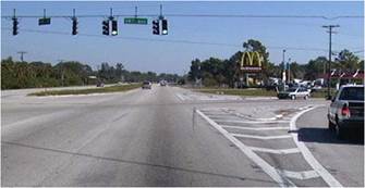
Figure 4.40: Uncoordinated Traffic Actuated (Code ‘2’) Example
These signals are typically identified by the presence of in-pavement loops or other detectors (intrusive or non-intrusive) on the approach to the intersection in one or more lanes.
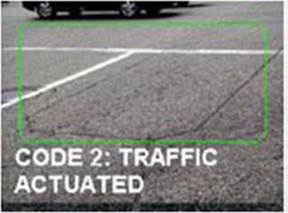
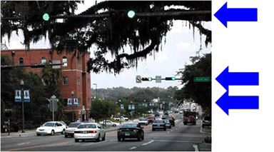
Figure 4.41: Coordinated Progressive (Code ‘3’) Example
These signals usually occur in high-traffic urban or urbanized areas, in close proximity to other signals (as shown in Figure 4.41), and are usually timed or coordinated with adjoining signals. This type of signal allows for a more constant free flow of traffic.
Description: The percent of green time allocated for through-traffic at intersections.
Use: For investment requirements modeling to calculate capacity and in congestion analyses.
Extent: All Sample Panel sections located in urban areas; optional for all other urban sections beyond the limits of the Sample Panel and rural Sample Panel sections.
Functional System |
1 |
2 |
3 |
4 |
5 |
6 |
7 |
|
|---|---|---|---|---|---|---|---|---|
NHS |
IH |
OFE |
OPA |
MiA |
MaC |
MiC |
Local |
|
Rural |
SP* |
SP* |
SP* |
SP* |
SP* |
SP* |
||
Urban |
SP |
SP |
SP |
SP |
SP |
SP |
SP |
|
SP = Sample Panel Sections SP* = Sample Panel Sections (optional) |
||||||||
Coding Requirements for Fields 8, 9, and 10:
Value_Numeric: Enter the percent green time in effect during the peak period (max peak period preferred) for through traffic at signalized intersections, for the inventoried direction of travel.
Value_Text: No entry required. Available for State Use.
Value_Date: No entry required. Available for State Use.
Guidance: Example – Procedure for Calculating Percent Green Time:
The timing of signals should occur during either the AM or PM peak period (i.e., 7-9 AM or 4-6 PM). Using a stopwatch, the entire signal cycle (green, amber, red) should be timed (in seconds), followed by the timing of the green cycle (in seconds). Then, divide the green cycle time by the entire signal time to find the percent green time. If the signal has a green arrow for turning movements, do not include the green arrow time in the timing of the green cycle. Use the average of at least three field-timing checks to determine a “typical” green time for traffic-actuated or demand responsive traffic signals.
Additional Guidance:
Code this Data Item for all sections where right and left turn data (Data Items 12 and 13) are coded.
For uncoordinated traffic actuated signals only, data can be collected when monitoring green time. Consider the surrounding environment and determine if the inventory direction of the signal would actually carry the peak flow for the intersection. Based on this approach, the value received may be an estimate depending upon the operation of the traffic signal during the peak hour. Furthermore, if the traffic signal is fully actuated, or the approach of interest is actuated, estimate the percent of green time based on the maximum green time available for that phase of operation versus the maximum cycle length. This would provide the “worst case” scenario since the volume on the actuated approach typically varies cycle by cycle.
Where peak capacity for a section is governed by a particular intersection that is on the section, this Data Item shall be coded based on the percent green time at that location; otherwise code this Data Item for the predominate intersection.
For traffic actuated traffic signals, use the results of a field check of several (three complete cycles) peak period light cycles to determine a “typical” green time. Ignore separate green-arrow time for turning movements.
Description: A count of at-grade intersections where traffic signals are present.
Use: For investment requirements modeling to calculate capacity and estimate delay.
Extent: All Sample Panel sections, optional for all other sections beyond the limits of the Sample Panel.
Functional System |
1 |
2 |
3 |
4 |
5 |
6 |
7 |
|
|---|---|---|---|---|---|---|---|---|
NHS |
IH |
OFE |
OPA |
MiA |
MaC |
MiC |
Local |
|
Rural |
SP |
SP |
SP |
SP |
SP |
SP |
||
Urban |
SP |
SP |
SP |
SP |
SP |
SP |
SP |
|
SP = Sample Panel Sections |
||||||||
Coding Requirements for Fields 8, 9, and 10:
Value_Numeric: Code the number of at-grade intersections where traffic signals are present, controlling traffic in the inventory direction.
Value_Text: No entry required. Available for State Use.
Value_Date: No entry required. Available for State Use.
Guidance: Only signals which cycle through a complete sequence of signalization (i.e., red, yellow (amber), and green) for all or a portion of the day shall be counted as a signal.
Access points to large traffic generators (e.g., shopping centers, malls, large work sites, office parks, apartment complexes, etc.) shall be counted as intersections if the access point is controlled by a traffic signal.
Special treatment is required when a Sample Panel section begins and/or ends with a traffic control device (i.e., Data Items 31, 32, and 33). This is accomplished by doing the following as illustrated in Figure 4.42:
For divided roadways, continuous cross streets are to be counted as a single intersection. If the cross street is not continuous and is separated by at least 50 feet, then it shall be counted as two intersections.
Roundabouts (see Figure 4.20) shall be coded under Data Item 33 (At-Grade/Other) intersections.
The sum of Data Items 31, 32, and 33 shall be equal to the total number of intersections on the section.
An Example of the Beginning or Ending Intersection Rule:
In the upper portion of Figure 4.42, 2 signalized intersections would be coded for this data item, when using either the beginning only or ending only rule. In the lower portion of Figure 4.42, when using the beginning only rule, 2 signalized intersections would be coded for this data item; when using the ending only rule, 1 signalized intersection would be coded for this data item.
Figure 4.42 Intersection Count Example
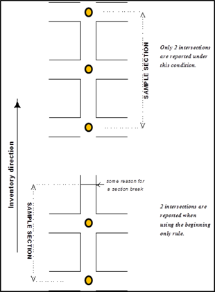
Description: A count of at-grade intersections where stop signs are present.
Use: For investment requirements modeling to calculate capacity and estimate delay.
Extent: All Sample Panel sections, optional for all other sections beyond the limits of the Sample Panel.
Functional System |
1 |
2 |
3 |
4 |
5 |
6 |
7 |
|
|---|---|---|---|---|---|---|---|---|
NHS |
IH |
OFE |
OPA |
MiA |
MaC |
MiC |
Local |
|
Rural |
SP |
SP |
SP |
SP |
SP |
SP |
||
Urban |
SP |
SP |
SP |
SP |
SP |
SP |
SP |
|
SP = Sample Panel Sections |
||||||||
Coding Requirements for Fields 8, 9, and 10:
Value_Numeric: Code the number of at-grade intersections where stop signs are present, controlling traffic in the inventory direction.
Value_Text: No entry required. Available for State Use.
Value_Date: No entry required. Available for State Use.
Guidance: A continuously operating (i.e. all day), flashing red signal shall be counted as a stop sign.
Stop signs on intersecting roads shall not be included in the total count.
Access points to large traffic generators (e.g., shopping centers, malls, large work sites, office parks, apartment complexes, etc.) shall be counted as intersections if the access point is controlled by a stop sign.
Special treatment is required when a Sample Panel section begins and/or ends with a traffic control device (i.e., Data Items 31, 32, and 33). This is accomplished by doing the following as illustrated in Figure 4.44:
For divided roadways, continuous cross streets are to be counted as a single intersection. If the cross street is not continuous and is separated by at least 50 feet, then it shall be counted as two intersections.
Roundabouts (see Figure 4.20) shall be coded under Data Item 33 (At-Grade/Other) intersections.
The sum of Data Items 31, 32, and 33 shall be equal to the total number of intersections on the section.
Figure 4.43 Stop Sign Controlled Intersection
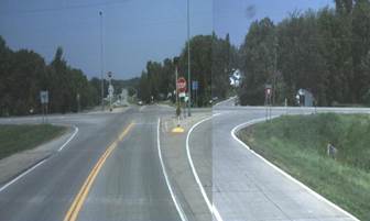
Source: MnDOT, Dec. 2012.
An Example of the Beginning or Ending Intersection Rule:
In the upper portion of Figure 4.44, 2 stop sign-controlled intersections would be coded for this data item, when using either the beginning only or ending only rule. In the lower portion of Figure 4.44, when using the beginning only rule, 2 stop sign-controlled intersections would be coded for this data item; when using the ending only rule, 1 stop sign-controlled intersection would be coded for this data item.
Figure 4.44 Intersection Count Example
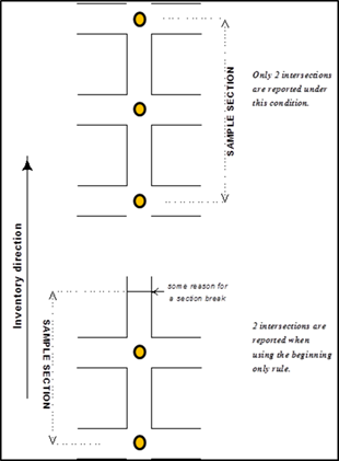
Description: A count of at-grade intersections, where full sequence traffic signal or stop sign traffic control devices are not present, in the inventory direction.
Use: For investment requirements modeling to calculate capacity and estimate delay.
Extent: All Sample Panel sections, optional for all other sections beyond the limits of the Sample Panel.
Functional System |
1 |
2 |
3 |
4 |
5 |
6 |
7 |
|
|---|---|---|---|---|---|---|---|---|
NHS |
IH |
OFE |
OPA |
MiA |
MaC |
MiC |
Local |
|
Rural |
SP |
SP |
SP |
SP |
SP |
SP |
||
Urban |
SP |
SP |
SP |
SP |
SP |
SP |
SP |
|
SP = Sample Panel Sections |
||||||||
Coding Requirements for Fields 8, 9, and 10:
Value_Numeric: Code the number of at-grade intersections where full sequence traffic signal or stop sign traffic control devices are not present, in the inventory direction.
Value_Text: No entry required. Available for State Use.
Value_Date: No entry required. Available for State Use.
Guidance:Intersections with either no traffic control devices, or specialized traffic control devices existing in the inventory direction, shall be included in the count for this data item.
Continuously operating (i.e. all day) flashing yellow signals and roundabouts (see Figure 4.20) shall be considered as an “at-grade/other” type of traffic control devices.
Access points to large traffic generators (e.g., shopping centers, malls, large work sites, office parks, apartment complexes, schools, etc.) shall be included in the evaluation for this Data Item.
Special treatment is required when a Sample Panel section begins and/or ends with a traffic control device (i.e., Data Items 31, 32, and 33). This is accomplished by doing the following as illustrated in Figure 4.46:
For divided roadways, continuous cross streets are to be counted as a single intersection. If the cross street is not continuous and is separated by at least 50 feet, then it shall be counted as two intersections.
The sum of Data Items 31, 32, and 33 shall be equal to the total number of intersections on the section.
Figure 4.45 At-Grade Other Example
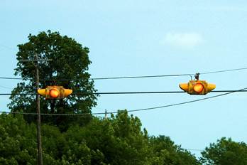
Source: Puckett Pages
An Example of the Beginning or Ending Intersection Rule:
In the upper portion of Figure 4.46, 2 at-grade other intersections would be coded for this data item, when using either the beginning only or ending only rule. In the lower portion of Figure 4.46, when using the beginning only rule, 2 at-grade other intersections would be coded for this data item; when using the ending only rule, 1 at-grade other intersection would be coded for this data item.
Figure 4.46: Intersection Count Example
Description: The measure of existing lane width.
Use: For investment requirements modeling to calculate capacity, estimate needed improvements, and compute a safety index, for cost allocation pavement models.
Extent: All Sample Panel sections, optional for all other sections beyond the limits of the Sample Panel.
Functional System |
1 |
2 |
3 |
4 |
5 |
6 |
7 |
|
|---|---|---|---|---|---|---|---|---|
NHS |
IH |
OFE |
OPA |
MiA |
MaC |
MiC |
Local |
|
Rural |
SP |
SP |
SP |
SP |
SP |
SP |
||
Urban |
SP |
SP |
SP |
SP |
SP |
SP |
SP |
|
SP = Sample Panel Sections |
||||||||
Coding Requirements for Fields 8, 9, and 10:
Value_Numeric: Enter the predominant through-lane width to the nearest whole foot.
Value_Text: No entry required. Available for State Use.
Value_Date: No entry required. Available for State Use.
Guidance: Lane width should be coded according to where the pavement/shoulder surface changes, or to the pavement lane striping (if the shoulder and pavement surface are the same).
Where there is no delineation between the through-traffic lane and the shoulder or parking lane, or where there is no centerline, estimate a reasonable split between the actual width used by traffic and the shoulder or parking lane based on State/local design guides.
When striping is placed inside the edge of the pavement (within approximately one foot) to keep traffic from breaking the pavement edge, ignore the striping and measure from the pavement edge to the center of a single centerline stripe. Or, if double centerline striping exists, measure to the center of the two stripes.
If more than one lane exists, measure all lanes in the inventory direction and use the average value to the nearest foot. If lane widths vary over the extent of the sample section, use the predominant width(s) for measuring and reporting purposes.
In Figure 4.47, the number of through lanes is 2; deducting 10 feet for parking on each side, which is either striped or from design practices, would leave width for two 18 foot lanes.
Figure 4.47: An Example for Measuring Lane Width
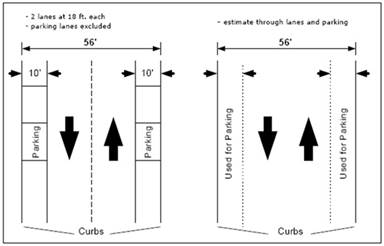
Description: The type of median.
Use: For investment requirements modeling to calculate capacity and estimate type of design and for national highway data base purposes.
Extent: All Sample Panel sections, optional for all other sections beyond the limits of the Sample Panel.
Functional System |
1 |
2 |
3 |
4 |
5 |
6 |
7 |
|
|---|---|---|---|---|---|---|---|---|
NHS |
IH |
OFE |
OPA |
MiA |
MaC |
MiC |
Local |
|
Rural |
SP |
SP |
SP |
SP |
SP |
SP |
||
Urban |
SP |
SP |
SP |
SP |
SP |
SP |
SP |
|
SP = Sample Panel Sections |
||||||||
Coding Requirements for Fields 8, 9, and 10:
Value_Numeric: Code the type of median using the following codes (Codes ‘5’ through ‘7’ are optional and shall be used if the data is available.):
Code |
Description |
|
|---|---|---|
1 |
None |
No median or unprotected area less than 4 feet wide. |
2 |
Unprotected |
Median exists with a width of 4 feet or more. |
3 |
Curbed |
Barrier or mountable curbs with a minimum height of 4 inches. |
4 |
Positive Barrier- unspecified |
Prevents vehicles from crossing median. |
5* |
Positive Barrier – flexible |
Considerable deflection upon impact. |
6* |
Positive Barrier – semi-rigid |
Some deflection upon impact. |
7* |
Positive Barrier – rigid |
No deflection upon impact. |
These definitions are summarized from AASHTO Policy on Geometric Design of Highways and Streets 2004.
* Codes 5, 6, and 7 are optional.
Value_Text: No entry required. Available for State Use.
Value_Date: No entry required. Available for State Use.
Guidance: Median - The portion of a divided highway separating the traveled way for traffic in opposing directions. The principal functions of a median are to:
A positive barrier normally consists of a guardrail or concrete barrier, but could consist of thick, impenetrable vegetation. All positive barrier medians, regardless of their width, must be considered for reporting purposes.
Turning lanes or bays are not considered medians unless the turning lanes/bays are cut into an existing median at intersections, site entrances (e.g., a shopping center), etc.; a continuous turning lane is not a median.
Figure 4.48: An Example of Median Type = 2, Unprotected
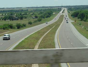
Source: TxDOT, Transportation Planning and Programming Division.
Description: The existing median width.
Use: For investment requirements modeling to calculate capacity and estimate type of design and for national highway data base purposes.
Extent: All Sample Panel sections, optional for all other sections beyond the limits of the Sample Panel.
Functional System |
1 |
2 |
3 |
4 |
5 |
6 |
7 |
|
|---|---|---|---|---|---|---|---|---|
NHS |
IH |
OFE |
OPA |
MiA |
MaC |
MiC |
Local |
|
Rural |
SP |
SP |
SP |
SP |
SP |
SP |
||
Urban |
SP |
SP |
SP |
SP |
SP |
SP |
SP |
|
SP = Sample Panel Sections |
||||||||
Coding Requirements for Fields 8, 9, and 10:
Value_Numeric: Enter the predominant median width including left shoulders, if any, measured between the inside edges of the left-most through lanes in both directions, to the nearest foot.
Value_Text: No entry required. Available for State Use.
Value_Date: No entry required. Available for State Use.
Guidance: Enter ‘99’ where the median width is 100 feet or greater.
The edge of through lane is determined by paint stripping, difference in pavement/shoulder construction material, or according to traffic use. If the median is raised or a ditch, do not add the contour as part of the median width measure.
For measurement purposes, ignore turning bays cut into the median.
Figure 4.49: An Example for Measuring Median Width
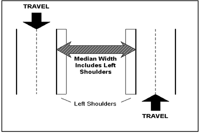
Figure 4.50: Median Width Measurement
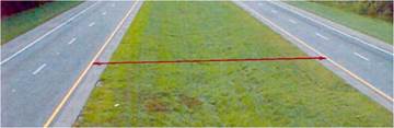
Source: FDOT RCI Field Handbook, Nov. 2008.
Description: The type of shoulder.
Use: For investment requirements modeling to estimate needed improvements.
Extent: All Sample Panel sections, optional for all other sections beyond the limits of the Sample Panel.
Functional System |
1 |
2 |
3 |
4 |
5 |
6 |
7 |
|
|---|---|---|---|---|---|---|---|---|
NHS |
IH |
OFE |
OPA |
MiA |
MaC |
MiC |
Local |
|
Rural |
SP |
SP |
SP |
SP |
SP |
SP |
||
Urban |
SP |
SP |
SP |
SP |
SP |
SP |
SP |
|
SP = Sample Panel Sections |
||||||||
Coding Requirements for Fields 8, 9, and 10:
Value_Numeric: Enter the code for the type of shoulder on the section.
Code |
Description |
|---|---|
1 |
None |
2 |
Surfaced shoulder exists – bituminous concrete (AC) |
3 |
Surfaced shoulder exists – Portland Cement Concrete surface (PCC) |
4 |
Stabilized shoulder exists (stabilized gravel or other granular material with or without admixture) |
5 |
Combination shoulder exists (shoulder width has two or more surface types; e.g., part of the shoulder width is surfaced and a part of the width is earth) |
6 |
Earth shoulder exists |
7 |
Barrier curb exists; no shoulder in front of curb |
Value_Text: No entry required. Available for State Use.
Value_Date: No entry required. Available for State Use.
Guidance: If the shoulder type varies over the extent of the section, code the predominant type. If left and right shoulder types differ on a divided facility, code the right shoulder type as the predominant type.
If there is a shoulder in front of a barrier curb, code this Data Item and Data Item 38 (Shoulder Width); do not code the area behind a barrier curb as a shoulder.
Disregard mountable curbs for HPMS reporting purposes. If there is a shoulder either in front of or behind a mountable curb, code this Data Item and Data Item 38 (Shoulder Width).
If a bike lane abuts the through lane, there cannot be a shoulder unless it is used as a combined shoulder/bike lane (sometimes indicated by signage or symbols on the pavement). If a bike lane or parking is completely separated from the roadway, it should not be considered.
If the section has parking abutting the through lane, there cannot be a shoulder. If there is parking on one side of a divided roadway and a shoulder or a curb on the other side, code this Data Item, Data Item 38 (Shoulder Width), and Data Item 40 (Peak Parking) accordingly. A shoulder cannot exist between a traffic lane and a parking lane.
Figure 4.51: Bituminous (Code ‘2’) Figure 4.52: Stabilized (Code ‘4’)
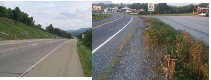
Figure 4.53: Combination (Code ‘5’) Figure 4.54: Earth (Code ‘6’)
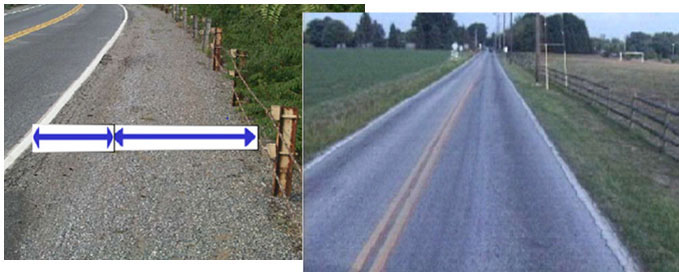
Figure 4.55: Barrier Curb / No Shoulder (Code ‘7’)
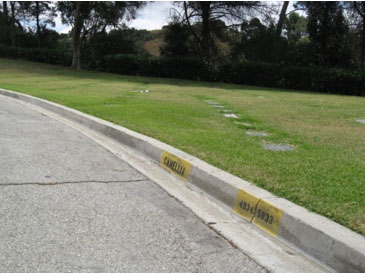
Description: The existing right shoulder width.
Use: For investment requirements modeling to calculate capacity and estimate needed improvements.
Extent: All Sample Panel sections, optional for all other sections beyond the limits of the Sample Panel.
Functional System |
1 |
2 |
3 |
4 |
5 |
6 |
7 |
|
|---|---|---|---|---|---|---|---|---|
NHS |
IH |
OFE |
OPA |
MiA |
MaC |
MiC |
Local |
|
Rural |
SP |
SP |
SP |
SP |
SP |
SP |
||
Urban |
SP |
SP |
SP |
SP |
SP |
SP |
SP |
|
SP = Sample Panel Sections |
||||||||
Coding Requirements for Fields 8, 9, and 10:
Value_Numeric: Enter the width of the right shoulder to the nearest whole foot.
Value_Text: No entry required. Available for State Use.
Value_Date: No entry required. Available for State Use.
Guidance: Do not include parking or bicycle lanes in the shoulder width as further illustrated in Figures 4.58-4.60.
Code the predominant width where it changes back and forth along a roadway section.
Ensure that the total width of combination shoulders is reported.
Include rumble strips and gutter pans in shoulder width.
This width shall be measured from the outer edge of the right-most through lane to the outer edge of the shoulder.
Figure 4.56: Earth Shoulder Measurement
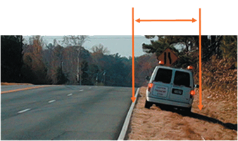
Earth Shoulder: Measure from the white stripe to the break point of the shoulder.
Figure 4.57: Bituminous Shoulder Measurement
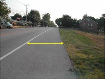
Bituminous Shoulder: Measure from the white stripe to the edge of the paved area.
Figure 4.58: Measuring Shoulders with Guardrails
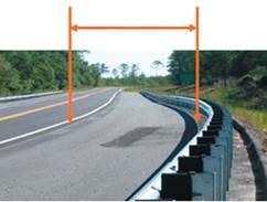
Guardrail Present on Shoulder: Measure from the edge of through lane to the face of the guardrail.
Figure 4.59: Measuring Shoulders with Parking/Bike Lanes
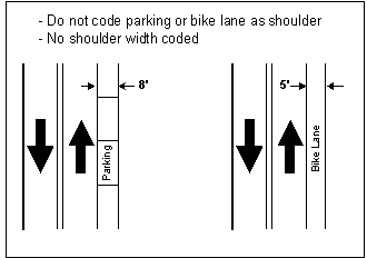
Figure 4.60: Measuring Shoulders with Parking and Bike Lanes
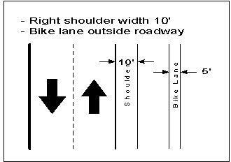
Figure 4.61: Measuring Shoulders with Combined Parking/Bike Lanes
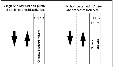
Description: The existing left shoulder width.
Use: For investment requirements modeling to calculate capacity and estimate needed improvements.
Extent: All Sample Panel sections, optional for all other sections beyond the limits of the Sample Panel.
Functional System |
1 |
2 |
3 |
4 |
5 |
6 |
7 |
|
|---|---|---|---|---|---|---|---|---|
NHS |
IH |
OFE |
OPA |
MiA |
MaC |
MiC |
Local |
|
Rural |
SP |
SP |
SP |
SP |
SP |
SP |
||
Urban |
SP |
SP |
SP |
SP |
SP |
SP |
SP |
|
SP = Sample Panel Sections |
||||||||
Coding Requirements for Fields 8, 9, and 10:
Value_Numeric: Enter the width of the left (median) shoulder to the nearest whole foot. Left shoulders shall only be coded for divided highway sections.
Value_Text: No entry required. Available for State Use.
Value_Date: No entry required. Available for State Use.
Guidance: Do not include parking or bicycle lanes in the shoulder width measurement.
Code the predominant width where it changes back and forth along a roadway section.
Ensure that the total width of combination shoulders is reported.
Include rumble strips and gutter pans in shoulder width.
This width shall be measured from the outer edge of the left-most through lane to the left-most edge of the inside shoulder.
Description: Specific information about the presence of parking during the peak period.
Use: For investment requirements modeling to calculate capacity.
Extent: All Sample Panel sections located in urban areas, optional for all other urban sections beyond the limits of the Sample Panel.
Functional System |
1 |
2 |
3 |
4 |
5 |
6 |
7 |
|
|---|---|---|---|---|---|---|---|---|
NHS |
IH |
OFE |
OPA |
MiA |
MaC |
MiC |
Local |
|
Rural |
||||||||
Urban |
SP |
SP |
SP |
SP |
SP |
SP |
SP |
|
SP = Sample Panel Sections |
||||||||
Coding Requirements for Fields 8, 9, and 10:
Value_Numeric: Enter the code that best reflects the type of peak parking that exists using the following codes:
Code |
Description |
|---|---|
1 |
Parking allowed on one side. |
2 |
Parking allowed on both sides. |
3 |
No parking allowed or none available. |
Value_Text: No entry required. Available for State Use.
Value_Date: No entry required. Available for State Use.
Guidance: Code this Data Item to reflect the permitted use, even if the section is not formally signed or striped for parking.
If parking is observed beyond the shoulder or the pavement-edge where there is no shoulder, use code ‘3.’
If parking lanes are legally used for through-traffic or turning lanes during the peak period, code the appropriate in-use condition.
Interstates and Freeways are usually assigned a code ‘3.’
Figure 4.62: Parking on One Side (Code ‘1’) Example
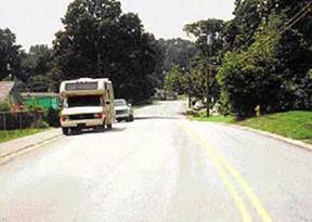
Source: FDOT RCI Field Handbook, Nov. 2008.
Figure 4.63: Parking on Both Sides (Code ‘2’) Example
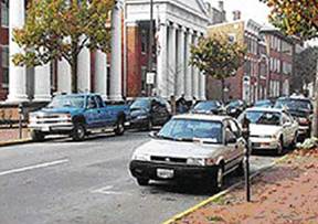
Source: FDOT RCI Field Handbook, Nov. 2008.
Figure 4.64: No parking allowed (Code ‘3’) Example
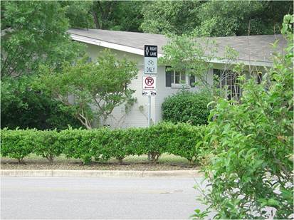
Source: TxDOT, Transportation Planning and Programming Division
Description: Obstacles that prevent widening of the existing roadway for additional through lanes.
Use: For administrative, legislative, analytical, and national highway database purposes.
Extent: All Sample Panel sections, optional for all other sections beyond the limits of the Sample Panel.
Functional System |
1 |
2 |
3 |
4 |
5 |
6 |
7 |
|
|---|---|---|---|---|---|---|---|---|
NHS |
IH |
OFE |
OPA |
MiA |
MaC |
MiC |
Local |
|
Rural |
SP |
SP |
SP |
SP |
SP |
SP |
||
Urban |
SP |
SP |
SP |
SP |
SP |
SP |
SP |
|
SP = Sample Panel Sections |
||||||||
Coding Requirements for Fields 8, 9, and 10:
Value_Numeric: No entry required. Available for State Use.
Value_Text: Code all conditions that apply in either direction on either side of the section and leave blank for unreported data using the following codes:
Code |
Definition |
Description |
|---|---|---|
X |
No obstacles |
No obstacles to widening. |
A |
Dense development |
Refers to the density and size of buildings to be acquired, the number of people that would need to be relocated, and the number of businesses that would need to be acquired. (Realizing dense development may be higher in urban areas; this should not be used as on obstacle for all urban areas and should be evaluated relative to the conditions in the area where the section is located). |
B |
Major transportation facilities |
Includes major rail lines, canals, airports, major natural gas and oil pipe lines whose location relative to the roadway section would limit expansion of the existing roadway. |
C |
Other public facilities |
Includes hospitals, museums, libraries, major public office buildings, schools, and universities. |
D |
Terrain restrictions |
Relates to geographic features that would make it very difficult to add lanes, requiring significant excavation, fill, or tunneling. This applies to both horizontal and vertical terrain restrictions. |
E |
Historic and archaeological sites |
Includes such things as historic buildings, historic land, large monuments, cemeteries, and known archaeological sites. |
F |
Environmentally sensitive areas |
Includes such areas as scenic landmarks, wetlands, bodies of water, areas inhabited or used by protected species. Scenic routes and byways are included in the category and are those national and State routes that have been identified and listed as official designations. |
G |
Parkland |
Includes National, State, and local parks. |
Value_Date: No entry required. Available for State Use.
Guidance: Enter any combination of the codes (e.g. if there are Historic and Dense development obstacles, code “EA” or “AE” for this Data Item). There is no requirement for the ordering of the codes; a code shall not be used more than once in a sequence of codes (e.g. “AEA”).
Code “X” cannot be used with other codes (e.g. “XE”)
This item provides for the coding of obstacles which may prevent or limit the ability to widen the roadway surface within approximately 100 feet of the outer edge of the through lanes that are present in either direction of the section.
If Data Item 42 (Widening Potential) is coded ‘8’ lanes or less, then this data item shall be coded “A” through “G”.
Figure 4.65: Cemetery (Code “E”) Obstacle Example 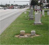 Source: PennDOT. |
Figure 4.66: Major Rail Line (Code “B”) Obstacle Example 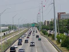 Source: TxDOT, Transportation Planning and Programming Division. |
Description: The number of through lanes that could be potentially added.
Use: For investment requirements modeling to estimate needed capacity improvements
Extent: All Sample Panel sections, optional for all other sections beyond the limits of the Sample Panel.
Functional System |
1 |
2 |
3 |
4 |
5 |
6 |
7 |
|
|---|---|---|---|---|---|---|---|---|
NHS |
IH |
OFE |
OPA |
MiA |
MaC |
MiC |
Local |
|
Rural |
SP |
SP |
SP |
SP |
SP |
SP |
||
Urban |
SP |
SP |
SP |
SP |
SP |
SP |
SP |
|
SP = Sample Panel Sections |
||||||||
Coding Requirements for Fields 8, 9, and 10:
Value_Numeric: Code the number of lanes (0-9) for which it is feasible to widen the existing road, in both directions. Code a ‘9,’ if it is possible to add nine or more lanes.
Value_Text: No entry required. Available for State Use.
Value_Date: No entry required. Available for State Use.
Guidance: Code this item based on how feasible it is to widen the existing road based on the presence of obstacles as identified in Data Item 41 (Widening Obstacles), and the proximity of the obstacle to the roadway. Consider medians, areas already within the existing right-of-way, and areas outside existing right- of- way to be available for widening.
Do not consider restrictions due to current right-of-way width, or projected traffic.
Narrowing lanes via restriping, resulting in an additional lane on a multilane facility does not constitute Widening Potential.
The cost of adding capacity to sections or corridors with limited Widening Potential is assumed to be significantly more costly than other more routine capacity improvements.
Figure 4.67: Widening Potential of 9 lanes (Max)  Source: PennDOT. |
Figure 4.68: No Widening Potential 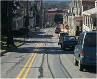 Source: PennDOT. |
Description: Curve classification data.
Use: For investment requirements modeling to calculate horizontal alignment adequacy and estimate running speed and operating costs.
Extent: All paved principal arterial and rural minor arterial Sample Panel sections; optional for all other sections beyond the limits of the Sample Panel.
Functional System |
1 |
2 |
3 |
4 |
5 |
6 |
7 |
|
|---|---|---|---|---|---|---|---|---|
NHS |
IH |
OFE |
OPA |
MiA |
MaC |
MiC |
Local |
|
Rural |
SP |
SP |
SP |
SP |
||||
Urban |
SP |
SP |
SP |
|||||
SP = Sample Panel Sections |
||||||||
Coding Requirements for Fields 8, 9, and 10:
Value_Numeric: Enter the total length of the segments that apply to each individual curve class, using the degree of curvature ranges listed in the table below. Each Sample Panel section will need to be subdivided to report the extent of each applicable curve class.
Curve Classification |
Degrees |
|---|---|
A |
Under 3.5 degrees (i.e., 0.061 radians) |
B |
3.5 – 5.4 degrees (i.e., 0.061 – 0.094 radians) |
C |
5.5 – 8.4 degrees (i.e., 0.096 – 0.147 radians) |
D |
8.5 – 13.9 degrees (i.e., 0.148 – 0.243 radians) |
E |
14.0 – 27.9 degrees (i.e., 0.244 – 0.487 radians) |
F |
28 degrees (i.e., 0.489 radians) or more |
Value_Text: No entry required. Available for State Use.
Value_Date: No entry required. Available for State Use.
Guidance: This information may be available from construction plans, GIS databases, and contracts for other data collection activities such as International Roughness Index (IRI) or pavement data, and video log.
The primary goal is to populate curve data for each paved sample on the applicable functional system. There are 6 classes of curvature (i.e., Curve Class A through Curve Class F). The beginning and ending points will remain constant for each of the data items; however the values for these data items will reflect the length of that particular curve class. Furthermore, the sum of the values for each of the 6 curve class Data Items must be equal to the total length of the entire sample.
Each curve and tangent segment is coded as a separate curve; segments are summed by curve class to obtain the total length in each class. Report the sum of the class lengths for each of the six curve classes (in units of miles); the sum of all curve lengths must equal the Sample Panel section length.
Example:
| Milepoint | 0.00 | 1.75 | 3.00 | 3.75 | 4.57 | 5.69 | |||||
|---|---|---|---|---|---|---|---|---|---|---|---|
|
|||||||||||
| Curve Length | 1.75 | 1.25 | 0.75 | 0.82 | 1.12 | ||||||
This example depicts a Sample Panel section for which the HPMS software would expect 4 records reported in the Sections dataset as depicted below:
2009|45|SCXXX|0|5.69|CURVES_A|5.69|1.75|||
2009|45|SCXXX|0|5.69|CURVES_B|5.69|1.25|||
2009|45|SCXXX|0| 5.69|CURVES_C|5.69|1.87|||
2009|45|SCXXX|0| 5.69|CURVES_E|5.69|0.82|||
Since no data exists for curve classes D and F in this example, there would not be a record reported for either class. Moreover, the value for Curve Class C is calculated by adding the values for both Curve Class C parts together. The beginning and ending points are consistent throughout all records within the sample. The sum of all of the Curve Class lengths must equal the total length of the Sample Panel section.
Figure 4.69 Curve Classification Example
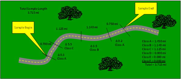
Source: TxDOT, Transportation Planning and Programming Division
Description: The type of terrain.
Use: For investment requirements modeling to calculate capacity and estimate needed capacity improvements and in the truck size and weight analysis process.
Extent: All principal arterial, minor arterial, and major collector Sample Panel sections located in rural areas, optional for all other rural sections beyond the limits of the Sample Panel.
Functional System |
1 |
2 |
3 |
4 |
5 |
6 |
7 |
|
|---|---|---|---|---|---|---|---|---|
NHS |
IH |
OFE |
OPA |
MiA |
MaC |
MiC |
Local |
|
Rural |
SP |
SP |
SP |
SP |
SP |
|||
Urban |
||||||||
SP = Sample Panel Sections |
||||||||
Coding Requirements for Fields 8, 9, and 10:
Value_Numeric: Enter the code that best describes the terrain according to the following table:
Code |
Description |
|---|---|
1 |
Level: Any combination of grades and horizontal or vertical alignment that permits heavy vehicles to maintain the same speed as passenger cars; this generally includes short grades of no more than 2 percent. |
2 |
Rolling: Any combination of grades and horizontal or vertical alignment that causes heavy vehicles to reduce their speeds substantially below those of passenger cars but that does not cause heavy vehicles to operate at crawl speeds for any significant length of time. |
3 |
Mountainous: Any combination of grades and horizontal or vertical alignment that causes heavy vehicles to operate at extremely low speeds for significant distances or at frequent intervals. |
Value_Text: No entry required. Available for State Use.
Value_Date: No entry required. Available for State Use.
Guidance: When coding this Data Item, consider the terrain of roadway sections that extend beyond the Sample Panel section limits, rather than solely the grade characteristics associated with the Sample Panel section. The extended roadway section may be several miles long and contain a number of upgrades, downgrades, and level sections. For long samples, such as rural freeway samples extending between interchanges, the extended roadway section and the Sample Panel section may be the same.
Figure 4.70 Level Terrain (Code ‘1’) Example 
Source: PennDOT. |
Figure 4.71 Rolling Terrain (Code ‘2’) Example
Source: PennDOT. |
Figure 4.72 Mountainous Terrain (Code ‘3’) Example
Source: PennDOT. |


