Field Evaluation of Detection-Control System

CHAPTER 4. DATA ANALYSIS RESULTS

INTRODUCTION

This chapter begins with descriptions of data collection sites because site details might help explain some of the findings. These details include drawings of the intersection geometry and tables of controller settings for the before and after conditions. The analysis of the actual crash data came near the end of the project. The goal of the traffic data collection was to determine propensity for running, vehicles caught in the dilemma zone, and max-outs. The Upper Limit Study used similar measures of effectiveness as studies 1 and 3. The following four studies were introduced in chapter1 and explained in chapter 2:

• Study 1: Performance Monitoring of Dilemma Zone Occupancy.

• Study 2: Before-After Crash Data Study.

• Study 3: Before-After Crash Surrogate Study.

• Study 4: Upper Limit Study.

DATA COLLECTION SITES

This chapter contains detailed site information on each of the eight sites to assist in better understanding the results. There is a site map showing geographic information followed by site schematics on each site to present the necessary details for understanding the geometric layout of the intersections and other detectors that were used for the before detection scenario. There is signal timing information on each site in both the before and after conditions. There is discussion about site, detection, and controller features that might have affected the outcome of the before-after comparison. The order of the site information in the remainder of this chapter is alphabetical. Florida (sites 1, 2, and 3) is first, followed by Illinois (sites 4 and 5), Louisiana (site6), and Texas (sites 7 and 8).

Sites 1, 2, and 3 Information

U.S. 27 is a north-south arterial that lies along the western edge of the city of Fort Lauderdale. The area to the west of U.S. 27 is mostly undeveloped swamps, and to the immediate east is urbanized residential development. Figure 4 shows a map of the local area showing these three intersections. The Pines intersection is a “T” intersection, whereas Griffin and Johnson are four-way intersections. All three intersections have two through lanes on the high-speed U.S. 27 approaches, and all have single left-turn and single right-turn lanes near the intersection. All three intersections have wide medians as shown in figure 5 through figure 7.

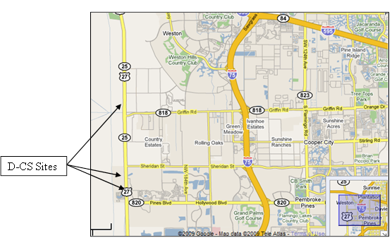
Original image: ©2009 Google® Tele Atlas; map annotations provided by TTI.

Figure 4. Map. Fort Lauderdale D-CS sites.⁽⁴⁾

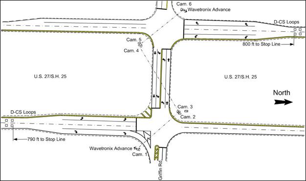
Figure 5. Map. Intersection layout at U.S. 27 and Griffin Rd.

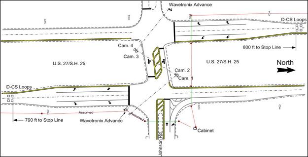
Figure 6. Map. Intersection layout at U.S. 27 and Johnson Rd.

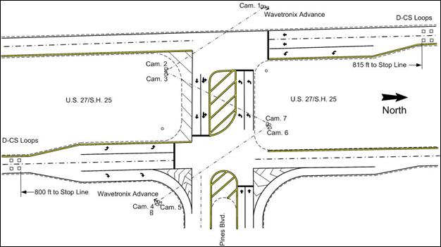
Figure 7. Map. Intersection layout at U.S. 27 and Pines Blvd.

Table 13 through table 18 summarize the controller settings for the three Florida intersections. Figure 8 and figure 9 show the signal phasing sequence for the Pines and Johnson intersections. The Griffin intersection had controller settings that were reasonably straightforward and did not use overlaps like the other two Florida intersections did. The signal phasing at the Pines intersection was an issue because D-CS needs the green phases on the main street approaches (NEMA phases 2 and 6) to begin simultaneously. BCT officials agreed to change the signal timing to cause these two phases to begin simultaneously and to eliminate one of the overlaps used previously. The other needed element was that the minimum green setting needed to conform to the D-CS recommended minimum of 15 s for approach speed limits of 55 mi/h or higher.⁽¹⁾ If there is no stop-line detection, the minimum green time must be at least sufficient to clear the stopped queue. There was no dilemma-zone detection in the before condition; the only detection used was stop-line detection.

The following definitions apply to table 13 through table 18 and other discussions of controller settings.

The following definitions apply to the before D-CS phase:

• MinGrn (minimum green, or initial green): The shortest possible vehicle green time before any added initial or vehicle extensions.⁽⁵⁾

• Passage (passage time, vehicle extension): When minimum green finishes timing, the green interval is allowed to extend for a length of time equal to maximum time in effect. Actual length of extension period depends on this phase vehicle extension time, frequency of vehicle actuations, and minimum gap setting.⁽⁵⁾

• Max1 and Max2: Maximum green time allowed in the presence of an opposing call. The higher-numbered maximum green selected will be in effect.⁽⁵⁾

• Yel (yellow change interval): the time that the phase yellow indication is displayed following a green indication.⁽⁵⁾

• Red Clearance Interval (or All-Red Interval): The interval at the end of the yellow change interval during which the phase has a red-signal display before the display of green for the following phase. Its purpose is to allow vehicles that entered the intersection on the yellow change interval to clear the intersection prior to the next phase.⁽⁶⁾

The following definitions apply to the after D-CS phase:^(1,7)

• TrapDist: TrapDist is the distance from the downstream end of the detector trap to the stop line of the intersection, in feet. The traps should be between 700 and 1,000 ft from the stop line.

• DZArrive: DZArrive is the travel time from the upstream end of the dilemma zone to the stop line, in seconds. The DZArrive time cannot be smaller than DZExit.

• DZExit: DZExit is the travel time from the downstream end of the dilemma zone to the stop line, in seconds. The DZExit time cannot be larger than DZArrival.

• Stage: The maximum green time is divided into two stages, stage 1 and stage 2. The Stage is the percentage of the maximum green time that is allocated to stage 1. Phase termination in stage 1 requires that all dilemma zones are clear. During stage 2, D-CS searches for a time when the number of vehicles in the dilemma zone is at a minimum.

• MaxSpeed (maximum speed): MaxSpeed is the maximum acceptable travel speed to be used by D-CS in mi/h. Speeds detected higher than this value are considered to be errors and are set to the maximum speed.

• MaxLength (maximum length): MaxLength is the maximum acceptable vehicle length for D-CS, in feet. Vehicle lengths reported to D-CS that are longer than the maximum length are considered to be errors, and the maximum length is reported instead.

• ZoneLength: ZoneLength is the measurement between the exit end of the upstream inductive loop and the exit end of the downstream inductive loop, in feet. The minimum zone length is 20 ft, although longer distances are also allowed.

Table 13. Controller settings U.S. 27/Griffin Rd.—before.

—No data.

Table 14. Controller settings U.S. 27/Griffin Rd.—after D-CS.

—No data.

Another issue in Florida was the maximum green setting in the Naztec 2070 controller after initiating the D-CS algorithm. The recommended range is 55 to 80 s, but the setting at Pines during field data collection was 50 s.⁽¹⁾ TTI did not check the settings because Naztec had been onsite to provide training and should have set up the controller properly. This error was discovered too late to change it during the field data collection at the Pines intersection. However, TTI checked the other intersections and set the value to 70 s at Griffin and Johnson. Even though the setting at Pines was lower than the recommended range, the result might still indicate how well it operates under these conditions.

Table 15. Controller settings for U.S. 27/Johnson Rd.—before D-CS.

—No data.

Table 16. Controller settings for U.S. 27/Johnson Dr.—after D-CS.

—No data.

Table 17. Controller settings for U.S. 27/Pines Blvd.—before D-CS.

—No data.

Table 18. Controller settings for U.S. 27/Pines Blvd.—after D-CS.

—No data.

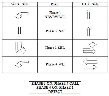
Figure 8. Chart. Phase sequence for U.S. 27/Pines Blvd.

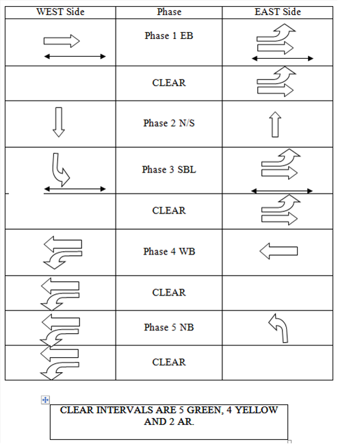
Figure 9. Chart. Phase sequence for U.S. 27/Johnson St.

Sites 4 and 5 Information

Illinois data collection followed Florida. The two Illinois sites were located east of Peoria on U.S. 24—one at the intersection with Cummings Lane and the other at the intersection with Main Street near Washington, IL. Figure 10 shows an area map indicating the location of the two Illinois sites. The two intersections had almost identical geometry, with two through lanes on each high-speed approach and single lane left-turn bays on each high-speed approach. Figure 11 and figure 12 show the intersection details. Table 19 through table 22 provide controller settings.

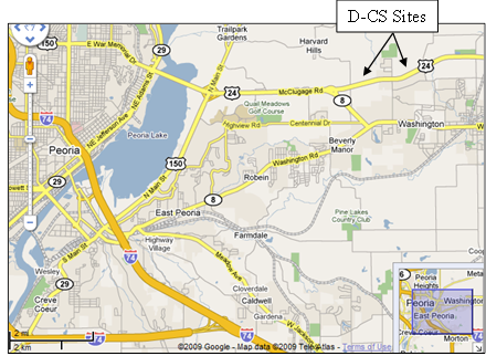
Original image: ©Google® Map Data 2009 Tele Atlas; map annotations provided by TTI.

Figure 10. Map. Washington, IL, D-CS sites.⁽⁸⁾

Challenges to Data Collection

IDOT used a single 6-ft by 6-ft inductive loop located about 5 s travel time upstream of the intersection for dilemma-zone detection at the Cummings and Main intersections. These loops were all still operational for collecting the before data. The distances from the D-CS loops to the stop line were 1,000 ft in all cases. Vehicular speeds at these sites adhered closely to the speed limit of 55 mi/h. Traffic at these intersections appeared to be primarily commuter traffic, with a pronounced peak in the morning and afternoon periods.

One of the challenges to the before data collection at the Illinois sites was loss of power, resulting in loss of some controller settings. Upon restoration of power, IDOT personnel noticed the problem with controller settings and worked with TTI personnel to get the appropriate settings reloaded. IDOT apparently set a relatively high value for passage time in the before condition to ensure clearance of the stopped queue, even though the only detector was 330 ft from the stop line. A question arose in trying to reset the passage time regarding how much time would be appropriate. TTI research personnel convinced IDOT to reduce it to 5 s.

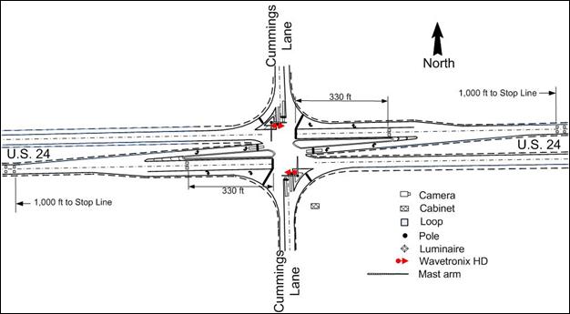
Figure 11. Map. Intersection layout at U.S. 24 and Cummings Ln.

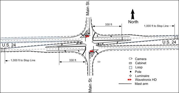
Figure 12. Map. Intersection layout at U.S. 24 and Main St.

Table 19. Controller settings for U.S. 24/Cummings Ln.—before D-CS.

—No data.

Table 20. Controller settings for U.S. 24/Cummings Ln.—after D-CS.

—No data.

Table 21. Controller settings for U.S. 24/Main St.—before D-CS.

—No data.

Table 22. Controller settings for U.S. 24/Main St.—after D-CS.

—No data.

Site 6 Information

Figure 13 shows an area map indicating the location of the Louisiana site, which is the intersection of LA 3235 and LA 3162. The location is near the small town of Galliano, LA, in the Lafourche Parish, about 60 mi south of New Orleans. LA 3235 is a high-speed roadway with speed limits on each approach at 55 mi/h, although observed local traffic speeds were higher. The D-CS approaches have two through lanes, a left-turn lane for the southbound approach, and a right-turn lane for the northbound approach. Three of the intersection legs serve general purpose traffic, and the fourth leg (eastbound) serves a casino and a convenience store. The only before detection at this intersection was at the stop line, so D-CS should significantly improve the safety of the intersection. Figure 14 shows the geometric layout of the intersection, indicating the location of detectors used for field data collection. Table 23 and table 24 provide controller settings for the before and after conditions.

A challenge at this site was an apparent conflict in the cabinet between the serial ports on the PC running the TTI software and the extra unused BIUs being turned on. After turning these extra BIUs off and operating with only the needed BIUs, the TTI data collection system ran normally. Solving this problem required an additional trip by one TTI person to meet Naztec personnel at the site. A second challenge was being able to monitor side street demand to determine how many legitimate max-outs occurred. In the before data collection, LaDOTD had set the main street phases to maximum recall (i.e., the main street phases were maxing out during each cycle of the day in the before data collection). LaDOTD was using an Autoscope™ mini-hub connected to the controller bus, which precluded the TTI equipment from monitoring the side street detectors in the after data collection. Therefore, determining the number of max-outs was not possible. However, the intersection functioned as it did prior to the installation of the D-CS equipment, which was important in determining before-after differences.

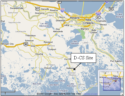
Original image: ©Google® Map Data 2009 Tele Atlas; map annotation provided by TTI.

Figure 13. Map. Louisiana D-CS site.⁽⁹⁾

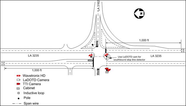
Figure 14. Map. Intersection layout at LA 3235 and LA 3162.

Table 23. Controller settings for LA 3235/LA 3162—before D-CS.

Table 24. Controller settings for LA 3235/LA 3162—after D-CS.

—No data.

Sites 7 and 8 Information

U.S. 281 at E. Borgfeld Drive in San Antonio

Figure 15 shows an area map indicating the location of the San Antonio site. The location is an isolated intersection north of the urbanized area surrounding San Antonio. Peak periods at this site indicated that a significant portion of the traffic was commuter traffic, with heavy inbound movement in the morning hours and heavy outbound movement during the late afternoon hours. This traffic was the heaviest of any of the D-CS data collection sites used in this project and was useful for conducting the Upper Limit Study.

Figure 16 shows the geometric layout of the intersection. The three-way intersection has two through lanes on the U.S. 281 approaches, while Borgfeld Drive has one lane in each direction away from the intersection. At the intersection, the northbound and eastbound approaches have left-turn bays. The U.S. 281 approaches had a series of seven inductive loops (each loop crossing both lanes) for dilemma-zone protection with distances from the stop line of 48, 93, 157, 239, 321, 425, and 534 ft. Table 25 through table 27 provide the controller settings for the original Eagle controller, the Naztec 2070 controller with the before settings, and the Naztec 2070 controller with the D-CS settings, respectively. Naztec representatives were supposed to enter settings in their controller (table 26) to replicate the operation of the original Eagle controller (table 25).

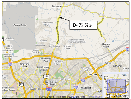
Original image: ©Google® Map Data 2009 Tele Atlas; map annotation provided by TTI.

Figure 15. Map. San Antonio, TX, D-CS site.⁽¹⁰⁾

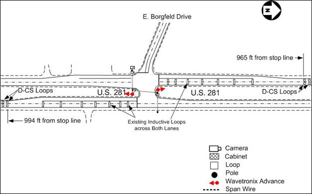
Figure 16. Map. Intersection layout at U.S. 281/E. Borgfeld Dr.

Table 25. Controller settings for U.S. 281/Borgfeld Dr.—before D-CS, Eagle controller.

—No data.

Table 26. Controller settings for U.S. 281/Borgfeld Dr.—before D-CS, Naztec controller.

—No data.

Table 27. Controller settings for U.S. 281/Borgfeld Dr.—after D-CS, Naztec controller.

—No data.

An important aspect of this site involved using the Naztec 2070 controller with a non-Naztec (Eagle) cabinet. Six of the eight sites involved in this research had Naztec controllers and cabinets, so this site offered a good opportunity to test the compatibility of this controller with a different cabinet (the other non-Naztec controller was at the Waco site, described below). During the initial installation of the Naztec controller for beginning data collection about May 30, 2009, the intersection went into flash mode when a detector BIU was unplugged. This occurrence could have been coincidental with removal of the BIU, but Naztec replaced the MMU anyway and was able to restore normal operation following this change.

TTI completed its normal data collection during the selected before/after period, which ended on July 27, 2009, before another problem occurred related to lightning (according to district personnel). The lightning strike again caused the intersection to go into flash mode. The Naztec controller had operated the intersection successfully for the 8-week period between the installation date of the Naztec controller and the lightning strike. As a temporary fix, district personnel replaced the Naztec controller with the original Eagle controller until Naztec could troubleshoot its 2070 controller. TxDOT shipped the controller back to Naztec during the week of August 17, 2009, to allow Naztec to troubleshoot the problem. Naztec found that the CPU board had been damaged; a technician from Naztec returned the repaired controller to the district on September 31, 2009. TTI reinstalled its monitoring equipment at the U.S.281/Borgfeld intersection on October 1, 2009, and began collecting data for the Upper Limit Study.

Upper Limit Study: TTI increased the maximum green setting in the D-CS 2070 controller on November 3, 2009, at the intersection of U.S. 281/Borgfeld to test its upper limit. At this intersection, Naztec and TTI set an initial maximum green of 75 s for phases 2 and 6. After some consideration of adding 80 and 85 s, TTI selected 85 and 95 s as the desired additional values to test because of the increased statistical significance in the greater spread.

U.S. 84 at Speegleville Road in Waco

Figure 17 shows an area map indicating the location of the Waco site, which is at the intersection of U.S. 84 and Speegleville Road. The location is southwest of Waco and outside the urban area. U.S. 84 is a high-speed roadway with a speed limit of 60 mi/h on each approach and a significant number of trucks. The D-CS approaches have two through lanes, single left-turn lanes, and single right-turn lanes. All four of the intersection legs serve general purpose traffic. Detection prior to installation of D-CS being installed consisted of a series of inductive loops upstream for dilemma-zone protection. Dilemma-zone detectors were 6-ft by 6-ft loops in each lane at 493, 267, and 111ft from the stop line. Through lanes on U.S. 84 had no stop-line detection, but left-turn bays did. Figure 18 shows the geometric layout of the intersection, indicating the location of detectors used for field data collection.

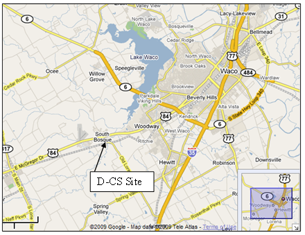
Original Image: ©Google® Map Data 2009 Tele Atlas; map annotation provided by TTI.

Figure 17. Map. Waco, TX, D-CS site.⁽¹¹⁾

The D-CS site in Waco had a NEMA TS1 cabinet, and City of Waco decisionmakers chose not to replace this cabinet with a TS2 cabinet to accommodate the D-CS, even though they were convinced that D-CS had made a significant difference in improving safety. On the first visit to this site, TTI researchers found that the PC running the D-CS algorithm had failed, so they prepared a replacement PC to be installed in the cabinet. Other TTI researchers had already wired the cabinet for a PC system, reducing the effort required to reinstall D-CS.

An issue that surfaced immediately following the reinstallation of D-CS at this site was due to not having stop-line detectors on through lanes. The City of Waco technicians had disconnected all previously installed dilemma-zone loops so that only the D-CS loops were connected for main street dilemma-zone protection. The D-CS algorithm does not start its search for gaps in the traffic stream until the termination of the minimum green in the controller. In this case, with the formation of long queues extending past the D-CS loops, the algorithm did not detect gaps appropriately, so it terminated the green phase prematurely with each cycle. The solution involved reconnecting the nearest inductive loops (located 111 ft from the stop line) and allowing the queue to begin clearing and for D-CS to function properly. With reconnection of the closest loops to the stop line, D-CS was able to function properly. At the first gap-out (or at the end of the minimum green setting, which was usually sooner), D-CS took over and started looking for gaps to safely end the green phase. Table 28 and table 29 provide the controller settings for the U.S. 84/Speegleville Road intersection.

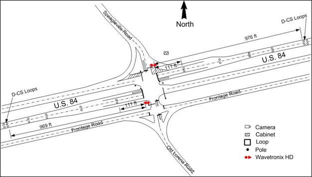
Figure 18. Map. Intersection layout at U.S. 84/Speegleville Rd.

Table 30 summarizes the speed limit and the dilemma-zone detection type used before installation of D-CS, stop-line detection, and distance to D-CS loops. Obviously, the best comparison of D-CS was with systems that had at least reasonably adequate dilemma-zone protection in the before condition. Therefore, the best comparisons are with Illinois and Texas sites.

Table 28. Controller settings for U.S. 84/Speegleville Rd.—before D-CS.

—No data.

Table 29. Controller settings for U.S. 84/Speegleville Rd.—after D-CS.

—No data.

Table 30. Site summary information.

¹Measured from stop line to trailing edge of exit loop.
²Single 6-ft by 6-ft loop located at 405 ft (about 5-s travel time) from stop line.
³City of Waco used distances from the stop line of 111, 267, and 493 ft.

TRAFFIC DATA ANALYSIS

Most of the results presented in this section were generated by human observers watching replay of recorded video of vehicles at each of the eight intersections. The monitoring system in each case involved a video camera/processor system to detect RLRs and a second (redundant) system that monitored vehicles caught in the dilemma zone. At each site, the process defined the dilemma zone as a range in travel time from 2 to 6 s. The redundant monitoring system consisted of two components: 1) the inductive loop pairs used for the D-CS, and 2) a Wavetronix™ Advance radar detector for each high-speed approach. The camera providing data to the video image processor also served as a surveillance camera to assist observers in verifying RLRs and vehicles in the dilemma zone. The inductive loops provided vehicle length and speed, and the radar detectors monitored speed and distance to each vehicle on the approach. TTI researchers were able to read the data stream from the radar detector’s serial port that updated speed and distance for each approaching vehicle every few milliseconds. This continuous stream of data provided enough information on approaching vehicles to serve as its own prediction of vehicles in the dilemma zone.

The following results are categorized according to the four studies. Studies 1 and 3 are similar, so results are combined into one section. Results from study 4, the Upper Limit Study, also come later in this section. Results from study 2 will come later in the final report at the end of the project because final crash data will not be available until that time.

Studies 1 and 3 Results

Table 31 and table 32 provide summary statistics describing the variables in the before-after database. The data in each row of either table reflect about 1 h of data collection for one signal phase at the associated intersection location. The data in table 31 indicate that the study observed more than 1,300 signal cycles at six locations. During these cycles, 88 vehicles entered the intersection within 6 s following the change in signal indication from yellow to red. Collectively, the intersections had both very low and very high traffic flow rates (120 to 1,512vehicles/h). They also experienced a wide range in cycle length (57 to 127 s). These wide ranges added a desired breadth in the range of conditions represented in the database.

As a first step in the analysis of the data, analysts computed red-light violation rates for each intersection approach, resulting in computation of two rates. The first rate is expressed in terms of red-light-running events per 1,000 vehicles. The second rate represents the number of red-light-running events per 10,000 vehicle-cycles, where “cycles” represents the average number of cycles per h during the period for which vehicles are counted. The use of “vehicle-cycles” is based on previous research demonstrating that exposure for red-light violations should be based on the count of vehicles and the count of cycles.⁽³⁾ Table 32 includes both of these rates.

The overall average rates at the study locations are 5.3 red-light violations per 1,000vehicles and 1.1 red-light violations per 10,000 vehicle-cycles. This number is the average for all sites where the rate in column 4 of table 32 is computed using total red-light running events divided by the total approach vehicles, and the rate in column 5 is computed using the equation in footnote C. The former rate is at the higher end of a range found in the literature (3.0 to 5.3 violations per 1,000 vehicles). Specifically, data reported by Kamyab et al. indicate an average rate of 3.0violations per 1,000vehicles.⁽⁶⁾ Data reported by Baguley indicate an average rate of 5.3violations per 1,000vehicles.⁽⁷⁾ Bonneson and Son reported 4.1 violations per 1,000 vehicles and 1.0 violations per 10,000 vehicle-cycles.⁽³⁾

Table 31. Before-after database summary—total observations.

¹Flow rate and counts include both passenger cars and heavy vehicles.
²Cycle length in the total rows represents an average length (not a sum).
³Percent change = 100 x (after/before - 1.0).
—Data not available.

Table 32. Before-after database summary—red-light-running violation rates.

¹Percent change = 100 x (after/before - 1.0).
²RLRs per 10,000 vehicle-cycles = count of red-light violations x 10,000 x Σ study hours / (Σ vehicles x Σ cycles).
*Values exceed the average rate by a factor of 2.0 or more.

The red-light violation rates listed in table 32 provide some indication of the extent of red-light violations at the intersections studied. The vehicle-based rates listed in column 4 indicate that three locations exceeded the average rate for the corresponding study period by a factor of 2.0 or more. The rates listed in column 5 indicate that three locations exceeded the corresponding average rate by 2.0 or more. Clearly, there is some discrepancy regarding which locations are the most problematic. This discrepancy illustrates the importance of considering both volume and number-of-cycles when computing the red-light violation rate for location-based comparison or evaluation. The vehicle-cycle-based rate logically represents a more reliable measure of the propensity for red-light violation than the vehicle-based rate because it accounts for two measures of exposure to a red-light violation.

Statistical Analysis Method

A preliminary examination of the data indicated that they are neither normally distributed nor of constant variance, as is assumed when using traditional least-squares regression. Under these conditions, the generalized linear modeling technique is appropriate because it accommodates the explicit specification of an error distribution using maximum-likelihood methods for coefficient estimation.

The distribution of violation frequency can be described as negative binomial because there are two different sources of variability. One source of variability stems from the differences in the mean frequency m among the otherwise similar intersection approaches. The other source stems from the randomness in frequency at any given site, which follows the Poisson distribution. The variance of the negative binomial distribution is seen in figure 19:

Figure 19. Equation. Variance of distribution.

Where:
V(x) is the variance of the distribution.

x is the observed violation frequency for a given approach having an expected frequency of E(m) and dispersion parameter k.

Researchers used the GENMOD regression procedure in the statistical analysis system software to estimate the model coefficients.⁽¹²⁾ This procedure is often used to calibrate regression models using count data with a large amount of variability (e.g., crash frequency).

Model Calibration

The regression analysis indicated that relationships existed between red-light violation frequency and exposure (expressed as the ratio of flow rate to cycle length), location, and the type of detection-and-control system used. Findings indicate that the regression coefficient associated with each of these factors was significant at a level of confidence that exceeded 95 percent. As a result of this analysis, the linear regression terms were specified in the model using the formulation in figure 20.

Figure 20. Equation. Expected red-light-running frequency.

Where:
E[R] = expected red-light-running frequency, vehicles/h.
Q = approach flow rate, vehicles/h.
C = cycle length, s.
I_Cummings = indicator variable (= 1.0 for U.S. 24/Cummings Lane location; 0.0 otherwise).
I_after = indicator variable (= 1.0 for data from the after study period, 0.0 otherwise).

This analysis also applied the equation shown to model dilemma-zone frequency and max-out frequency. In each case, the process substituted the corresponding dependent variable for E[R] in figure 20.

Red-Light Violation Model Results

The regression analysis indicated that the calibrated model accounted for most of the variability in the data. The U.S.24/Cummings Lane location required one location-specific indicator variable because this location experienced less than one-half of the violations of the other locations, all other factors considered. The model variables explain the differences among the other locations.

Table 33 shows the statistics related to the calibrated red-light-running model. The calibrated coefficient values can be used with figure 20 to predict the hourly red-light-running frequency for a given intersection approach. The analysis found that a dispersion parameter k of 54.9 yielded a scaled Pearson χ² statistic for the model is 25.7, and the degrees of freedom are 24 (= n-p-1 = 28-3-1). Because this statistic is less than χ²_{0.05, 24} (= 36), the hypothesis that the model fits the data cannot be rejected. A measure of model fit that is appropriate for negative binomial error distributions is R_K², as developed by Miaou.⁽¹³⁾ The interpretation of this statistic is the same as for the coefficient of determination R² (i.e., that values near 1.0 suggest a very good fit to the data). R_K² for the calibrated model is 0.98.

Table 33. Calibrated red-light violation model statistical description.

The last rows of table 33 list the regression coefficients for the model. The t-statistic shown indicates that all coefficients are significant at a 95-percent level of confidence or higher. A negative coefficient for b₃ indicates that red-light violations were less frequent during the after period. Based on the model structure, this coefficient can be converted into an equivalent reduction percentage of 82 percent (= 100 [1 - e^−1.733]). Thus, the analysis indicates that the after study periods experienced 82 percent fewer red-light violations than the before study periods. This reduction factor is consistent with the average change in violation rates shown at the bottom of table 32.

Researchers assessed the fit of the model through the graphical comparison of the observed and predicted red-light-running frequencies as shown in figure 21. The trend line in this figure does not represent the line of best fit; rather, it is a “y = x” line. The data would fall on this line if the model predictions exactly equaled the observed data. The trends shown in this figure indicate that the model is able to predict the red-light violation frequency without bias.

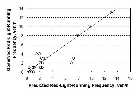
Figure 21. Graph. Comparison of observed and predicted red-light-running frequency.

Dilemma Zone Model Results

The model used for the dilemma-zone frequency analysis was the same as used for the red-light violation model. The regression analysis indicated that the calibrated model accounted for most of the variability in the data. Again, one location-specific indicator variable was needed to account for the U.S.24/Cummings Lane location. This location experienced less than one-half of the dilemma-zone count compared with the other locations, all other factors considered. The model variables explain differences among the other locations.

Table 34 shows the statistics related to the calibrated dilemma zone model. The calibrated coefficient values can be used with figure 20 to predict the hourly number of vehicles in the dilemma zone at yellow onset for a given intersection approach. A dispersion parameter k of 6.2 yielded a scaled The Pearson _X2 statistic for the model is 19.7 and the degrees of freedom are 20 (= n-p-1 = 24-3-1). Because this statistic is less than 2 0.05, 20 (= 26), the hypothesis that the model fits the data cannot be rejected. R_K² for the calibrated model is 0.87. This value suggests that the model explains most of the variability in the data.

The last rows in table 34 show the regression coefficients for the model. The t-statistic shown indicates that all coefficients are significant at a 95-percent level of confidence or higher. A negative coefficient for b₃ indicates that there were fewer vehicles caught in the dilemma zone during the after period. Based on the model structure, this coefficient can be converted into an equivalent reduction percentage of 73 percent (= 100 [1 - e^−1.317]). Thus, the analysis indicates that the after study periods experienced 73 percent fewer vehicles in the dilemma zone than the before study periods.

Table 34. Calibrated dilemma zone model statistical description.

Researchers assessed the fit of the model through the graphical comparison of the observed and predicted dilemma-zone counts as indicated in figure 22. The trend line in this figure does not represent the line of best fit; rather, it is a “y = x” line. The data would fall on this line if the model predictions exactly equaled the observed data. The trends shown in this figure indicate that the model is able to predict the dilemma-zone count without bias.

Max-Out Model Results

The model used for the max-out frequency analysis was the same as used for the red-light violation model. The regression analysis indicated that the calibrated model accounted for most of the variability in the data. The U.S.24/Cummings Lane location required one location-specific indicator variable. This location experienced very few max-outs relative to the other locations. Model variables explain differences among the other locations.

Table 35 shows the statistics related to the calibrated max-out model. The calibrated coefficient values can be used with figure 20 to predict the hourly max-out frequency for a given intersection approach. A dispersion parameter k of 0.43 yielded a scaled Pearson χ² of 1.19. The Pearson χ² _{0.05, 22} (= 34), the hypothesis that the model fits the data cannot be rejected. R_K² for the calibrated model is 0.72. This value suggests that the model explains much of the variability in the data.

The last rows of table 35 show the regression coefficients for the model. The t-statistic shown indicates that all coefficients but one are significant at a 95-percent level. The coefficient b₃ for “effect of a change in detection and control” was not statistically significant.

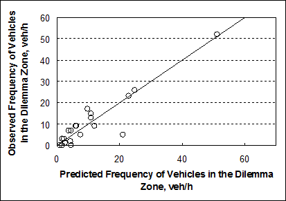
Figure 22. Graph. Comparison of observed and predicted number of vehicles in the dilemma zone.

Table 35. Calibrated max-out model statistical description.

A negative coefficient for b₃ indicates that max-outs were less frequent during the after period. Based on the model structure, this coefficient can be converted into an equivalent reduction percentage of 51 percent (= 100 [1 - e^−0.722]). Thus, the analysis indicates that the after study periods experienced 51 percent fewer max-outs than the before study periods. However, this percentage varied widely among locations, and it was relatively infrequent at all locations (except the U.S. 84/Speegleville Road location). For these reasons, it appears that the change in detection and control reduces max-out frequency, but the trend is not known with certainty. The available data make it impossible to rule out the possibility that the max-out frequency actually increased in the after period.

Researchers analyzed the fit of the model through the graphical comparison of the observed and predicted max-out frequencies as indicated in figure 23. The trend line in this figure does not represent the line of best fit; rather, it is a “y = x” line. The data would fall on this line if the model predictions exactly equaled the observed data.

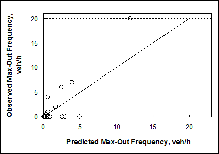
Figure 23. Graph. Comparison of observed and predicted max-out frequency.

Study 4 Results

Table 36 summarizes the findings of the upper limit comparison of different maximum green settings of 75, 85, and 95 s. The results indicated in this tabular summary are followed by statistical analysis. Visual observation of the results does not make a compelling case indicating improvement in the standard MOEs except for phase 6 max-outs. Phase 2 max-outs remain constant because the northbound through movement is impeded less often (only by phase 8) than phase 6. There is no apparent trend in RLRs from these data.

Table 36. Upper Limit Study summary.⁽¹⁾

¹AM peak 6–9; PM peak 4–8.
Blank cell = base condition.
EOP = evening off peak.
EP = evening peak.
LL = left lane.
MOP = morning off peak.
MP = morning peak.
RL = right lane.

Table 37 provides summary statistics describing the variables in the upper-limit database. The data in each row of this table reflect about 1 h of data collection for 1 signal phase at the U.S.281/E. Borgfeld Drive location. The data in table 37 indicate that the research project observed more than 300 signal cycles at this location. During these cycles, the subject phase terminated by max-out for 14 signal cycles. The traffic flow rate ranged from 1,255 to 1,450vehicles/h, and the cycle length ranged from 91 to 109 s.

The last column of table 37 indicates that the sample size is somewhat small, having only 14observations during the collective set of study hours. The trend in the data (shown in the last few rows of the last column) indicates that the max-out frequency decreased with increasing maximum green duration. The number of max-outs decreased by 43 percent when operating the intersection with an 85-s maximum green compared with a 75-s maximum green. The number of max-outs decreased 57 percent when operating at a 95-s maximum green, compared with a 75-s maximum green.

Table 37. Upper-limit database summary—total observations.

¹Flow rate and counts include both passenger cars and heavy vehicles.
²Cycle length in the total rows represents an average length (not a sum).
³Percent change = 100 x (after/before - 1.0).

The statistical analysis used a model similar to figure 20 but with an additional variable for maximum green duration. The results of this analysis indicate that the trend in the last column of table 37 was not statistically significant. Thus, it appears that a longer maximum green setting may reduce max-out frequency, but the trend is not known with certainty. The available data make it impossible to rule out the possibility that the max-out frequency actually increases with maximum green duration.

The original intent for the Upper Limit Study was to compare the MOEs—red-light running, vehicles caught in the dilemma zone, and max-out frequency—to those caused by traditional detection, accounting for any variations in traffic or other conditions. The only comparison that was available for this intersection was comparing the before data from the existing inductive loops with the after data with D-CS, both with Max1 set at 75 s, which was done in the earlier comparisons. Further analysis using simulation would be the only way to evaluate the desired increase in demand and determine at what volume D-CS is no longer able to provide adequate dilemma-zone protection.

Study 2 Results

The primary objective of study 2 was to evaluate before-after crash data to determine the effectiveness of D-CS in reducing motor vehicle crashes at signal-controlled intersections. The section reports on a statistical analysis to evaluate the effectiveness that D-CS had on all (TOT), fatal and injury (FI), and angle plus rear end (angle plus RE) crashes. The reason some categories were combined was to increase the sample size.

Methodology

The research team used a before-after study to evaluate the safety effectiveness of D-CS at the eight selected sites. The evaluation used the comparison group method with correction for traffic flow to overcome some of the problems with a simple or naïve before-after study. This method uses a comparison group that has influencing factors similar to those of the treated group. The following assumptions underlie this approach:⁽¹³⁾

• The factors that affected safety have changed in the same way from before the improvement to after the improvement for both the treatment and the control groups.

• The changes in the various factors influence the safety of the treatment and the control groups in the same manner.

The results from this approach are considered more accurate and reliable than the simple before-after study because the new approach can account for external causal factors. Although this approach can improve the weakness of the simple method through careful selection ofng the comparison groups, it is still subject to the regression-to-the-mean (RTM) bias because it predicts the expected number of target crashes of a site based on the before-period crash number only. RTM refers to the tendency for a fluctuating characteristic of an entity to return to a typical value in the period after an extraordinary value has been observed.⁽¹⁶⁾

The comparison group method considers only the factors that are unidentified, unmeasured, and not understood.⁽¹⁴⁾ If a before-after study is planned, information about traffic flow in the before and after periods should always be secured.⁽¹⁴⁾ Because the effect of change in traffic flow on safety may be large, it is important to try to account for it directly and explicitly. Harwood et al. used a variation of the comparison group approach, which makes the traffic volume adjustment using a regression relationship between crash frequency and traffic volume. The before-after study uses the following steps:⁽¹⁶⁾

Step 1. Define the target crashes.

Safety of D-CS is measured in terms of its ability to reduce crashes related to phase termination (e.g., rear-end and angle crashes). The target crashes are the types of crashes that are likely influenced by D-CS.

Step 2. Define the comparison group.

The comparison group method uses sites that are similar to the treated entities but without D-CS installation. Comparison group crashes are useful in explaining factors other than D-CS that might have influenced the safety of an intersection. In each case, the operating agency offered sites that were similar to the treated sites.

Step 3. Predict the expected number of crashes and variances for after period.

This information is required to account for factors other than the treatment that affect safety but are either not measured or the influence of which on safety is not known. The expected number of after period crashes and their variance for site i had the treatment not been implemented at the treated site is shown in figure 24:

Figure 24. Equation. Expected number of crashes and variances for after period.

Where:
_a = the ratio of duration of after period to the duration of before period.
_r= the ratio of after to before target crashes at comparison sites = (N/M)/(1=1/M).
_tf = the ratio of the functional relationship between traffic flow and safety in the before period to that in the after period = f(A_avg)/f(B_avg).
K = total crash counts during the before period in a treated site.
M = total crash counts during the before period in a comparison site.
N = total crash counts during the after period in a comparison site.
A_avg = expected traffic volume (averaged over the number of years) in the after period.
B_avg = expected traffic volume (averaged over the number of years) in the before period:

Step 4. Compute the sum of the predicted crashes over all treated sites and its variance.

It is widely recognized that the safety effect of a treatment varies from one site to another. Thus, instead of a single site, one would like to know the average safety effect of the treatment for a group of sites. The expected number of after-period crashes and their variances for a group of sites had the treatment not been implemented at the treated sites is given in figure 25:

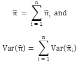
Figure 25. Equation. Sum of predicted crashes and its variance.

Step 5. Compute the sum of the actual crashes over all treated sites.

For a treated site, the crashes in the after period are influenced by the implementation of the treatment. The safety effectiveness of a treatment is known by comparing the actual crashes with the treatment to the expected crashes without the treatment. The actual number of after-period crashes for a group of treated sites is given in figure 26:

Figure 26. Equation. Sum of actual crashes for treated sites after period.

Where:
L_i = total crash counts during the after period at site i.

Step 6. Compute the unbiased estimate of safety-effectiveness of the treatment and its variance.

The “index of effectiveness (θ)” is defined as the ratio of what safety was with the treatment to what it would have been without the treatment. The parameter gives the overall safety effect of the treatment and is seen in figure 27.

Figure 27. Equation. Index of effectiveness.

The percent increase in the number of target crashes owing to the treatment is calculated by 100(1 - ) percent. If is less than 1, then the treatment has a positive safety effect. The estimated variance and standard error of the estimated safety-effectiveness are shown in figure 28 and figure 29:

Figure 28. Equation. Variance of estimated safety-effectiveness.

Figure29. Equation. Standard error of safety-effectiveness.

The approximate 95-percent confidence interval for θ is given by adding and subtracting 196s.e.() to . If the confidence interval contains the value 1, then no significant effect has been observed.

Data Description

Table 38 summarizes the number of crashes occurring in the four States by the following metrics:

• Treatment period (before D-CS and after D-CS).

• Length of analysis period (duration in years).

• TOT crashes.

• Severity of crashes (FI).

• Type of crashes related to D-CS (angle plus RE).

All sites except one (U.S. 281/E. Borgfeld in Texas) have a comparison site, although in most cases, more than one treatment site uses the same nearby comparison site.

Table 38. Number of crashes at treatment and comparison sites.

AADT = annual average daily traffic.
N/A = not applicable.

Analysis Results

Safety performance functions (SPF) are used to develop a relationship between the number of crashes and daily traffic data. This study develops the SPFs with the crash and traffic data in the before period. Table 39 shows the summary of statistics for these crashes and annual average daily traffic (AADT). The number of observations is not the number of intersections independent spatially but the number of intersections independent temporally (e.g., a year). As a result, an intersection may produce several data points depending on the number of years of data collected.

Table 39. Summary statistics of crashes and traffic flow.

—No data.

The Poisson-gamma (i.e., negative binomial) model is the most common type of model used by transportation safety analysts for modeling traffic crashes. This model is preferred over other mixed-Poisson models because the gamma distribution is the conjugate of the Poisson distribution. The Poisson-gamma model has the following model structure: the number of crashes Y_it for a particular i^th site and time period t when conditional on its mean µ_it Poisson distributed and independent over all sites and time periods, as shown in figure 30

Figure 30. Equation. Number of crashes based on the Poisson-gamma model.

Where:
i = 1, 2, …, i, and t = 1, 2, …, t
The mean of the Poisson is structured as shown in figure 31:

Figure 31. Equation. Mean of the number of crashes.

Where:
f = function of the covariates (X).
β = vector of unknown coefficients.
e_it is the model error independent of all the covariates.

The functional form used for the model in this study is as shown in figure 32:

Figure 32. Equation. Functional form of safety performance.

Where:
Y = number of years of crash data.
β_i = a vector of unknown coefficients (to be estimated) (i = 0,1).

Table 40 summarizes the estimation results for all three crash types. In general, the sign and magnitude of the regression coefficients in table 40 are logical and consistent with previous research findings.

Table 40. Parameter estimation for SPF.

The coefficients in table 40 were combined with the equation in figure 32 to obtain the crash mean of each crash type:

The form of each model is shown in figure 33, figure 34, and figure 35:

Figure 33. Equation. SPF for TOT crashes.

Figure 34. Equation. SPF for FI crashes.

Figure 35. Equation. SPF for angle plus RE crashes.

Safety Effects of D-CS

Table 41 presents the average safety effect of D-CS based on crash data. The average safety effect of D-CS is known from the unbiased estimate of index of effectiveness (). If this value is less than 1, then D-CS has a positive effect on safety (improves safety). The analysis results suggest that D-CS has no effect on TOT and FI crashes and produces a reduction of 9 percent for angle plus RE crashes. The standard deviation of this estimate of average safety effect is 15percent, so at a 95-percent confidence level, the result is not significant. This result can be attributed to the small sample size. Achieving a significant result at the 5-percent level would require a larger number of treated sites, a longer period of crash data collection, or both.

Table 41. Average safety effect of D-CS based on crash data.

¹A negative value represents a decrease, while a positive value represents an increase in crashes.