
Emission rates can vary widely with vehicle speed. Figure 1 shows the "speed correction factors" used in MOBILE6 for freeways for Tier 1 vehicles, which are used to scale emission rates from their base value (at 19.6 mph) to a value appropriate for a given speed. Per mile emission rates for particulate matter from exhaust and break and tire wear do not vary with speed in MOBILE6.
Figure 1: MOBILE6 Speed Correction Factors for Freeways (Tier 1 vehicles)
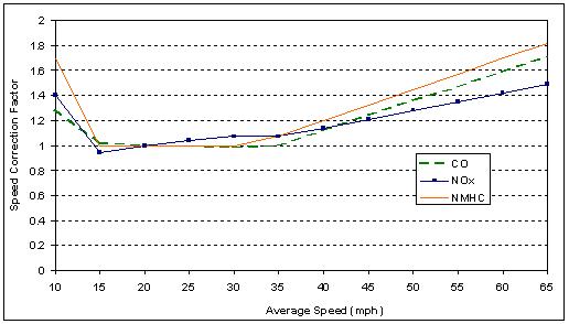
Source: Facility Specific Speed Correction Factors, Draft, U.S. EPA, Report Number M6.SPD.002, August 1999.
To account for the effects of speed, MOBILE6 calculates emission rates that are specific to each speed grouping (called "speed bin"). The speed bins are defined in 5 mph increments. When developing area-wide emissions estimates, users typically input the share of VMT that occurs at the different speed levels, and MOBILE6 then weights the speed-specific emission rates by VMT to produce a composite emission factor.
MOBILE6 accounts for speed effects by calculating emission rates specific to each speed, then weighting the speed-specific emission rates by VMT to produce a composite emission factor (by facility type). Thus, when developing area-wide emissions estimates, users have the option of inputting the fraction of VMT that occurs at the different speed levels, or rely on the model default values for the distribution of VMT by speed. The necessary level of detail of speed information supplied by the model user depends on local conditions and the intended uses of the emissions estimates (e.g., area-wide inventory vs. photochemical modeling).
VMT Distribution by Speed and by Hour (most detailed)
The greatest level of detail a user can provide for speed information is to specify the distribution of VMT by speed and by hour of day. This is accomplished using the SPEED VMT command in MOBILE6. For each hour of the day, the user provides the fraction of VMT that occurs in each of 14 speed "bins," shown in Table 1.
| Number | Abbreviation | Description |
|---|---|---|
| 1 | 2.5 mph | Average speeds 0-2.5 mph |
| 2 | 5 mph | Average speeds 2.5-7.5 mph |
| 3 | 10 mph | Average speeds 7.5-12.5 mph |
| 4 | 15 mph | Average speeds 12.5-17.5 mph |
| 5 | 20 mph | Average speeds 17.5-22.5 mph |
| 6 | 25 mph | Average speeds 22.5-27.5 mph |
| 7 | 30 mph | Average speeds 27.5-32.5 mph |
| 8 | 35 mph | Average speeds 32.5-37.5 mph |
| 9 | 40 mph | Average speeds 37.5-42.5 mph |
| 10 | 45 mph | Average speeds 42.5-47.5 mph |
| 11 | 50 mph | Average speeds 47.5-52.5 mph |
| 12 | 55 mph | Average speeds 52.5-57.5 mph |
| 13 | 60 mph | Average speeds 57.5-62.5 mph |
| 14 | 65 mph | Average speeds >62.5 mph |
The distribution of VMT by speed will vary by roadway functional class. The four functional classes in MOBILE6 are as follows:
MOBILE6 allows users to enter a distribution of VMT by speed only for freeways and arterials/collectors. For local roadways and freeway ramps, the average speed in the model is fixed at 12.9 mph and 34.6 mph, respectively, and cannot be modified. Thus, a MOBILE6 user that provides the most detailed local speed information possible will input a 24 x 14 x 2 matrix of VMT fractions (24 hours in the day, 14 speed bins, 2 facility types). EPA recommends that local estimates at this level of detail be developed for non-attainment areas that are classified as moderate or above and that are required to perform photochemical modeling. Most small urban and rural areas are not expected to provide this level of detail, and most are unlikely to have the data necessary to develop such inputs.
VMT Distribution by Speed
A simpler option is to provide localized data for VMT fractions by speed bin for an entire 24-hour period (i.e., no local information on variation by hour of day). For the development of an on-road emission inventory or forecast for SIP or conformity purposes, EPA expects nonattainment areas that are classified as moderate or above to use their own such specific estimates of VMT by average speed.[11]
This option might be used, for example, by a region that runs a travel demand forecasting (TDF) model for a 24-hour period, but has little data on how the VMT distribution by speed varies by hour of the day. The TDF model will provide the VMT and speed on every modeled link. Using the modeled speed (or some other derivation of speed), the VMT on each link is assigned to one of the 14 speed bins (separately for freeways and for arterials/collectors). The VMT in each speed bin is then divided by the sum of all the VMT to calculate the VMT fractions.
As an illustration, Table 2 shows the VMT and VMT fractions by speed bin for freeways and arterials used for a 1995 inventory for Ada County, Idaho. In this example, most freeway VMT occurs in the 47.5 mph to 62.5 mph range and most arterial VMT occurs in the 27.5 mph to 37.5 mph range.
| VMT | VMT Fraction | |||
|---|---|---|---|---|
| Speed Bin (mph) | Freeway | Arterial | Freeway | Arterial |
| 0.0 -2.5 | 0 | 0 | 0 | 0 |
| 2.5 -7.5 | 0 | 0 | 0 | 0 |
| 7.5 - 12.5 | 0 | 0 | 0 | 0 |
| 12.5 - 17.5 | 147 | 5 | 0.0018 | 0.0000 |
| 17.5 - 22.5 | 230 | 1,669 | 0.0027 | 0.0098 |
| 22.5 - 27.5 | 2,318 | 7,720 | 0.0277 | 0.0454 |
| 27.5 - 32.5 | 468 | 56,278 | 0.0056 | 0.3309 |
| 32.5 - 37.5 | 0 | 67,940 | 0 | 0.3995 |
| 37.5 - 42.5 | 0 | 15,866 | 0 | 0.0933 |
| 42.5 - 47.5 | 7,407 | 20,578 | 0.0885 | 0.1210 |
| 47.5 - 52.5 | 42,903 | 0 | 0.5128 | 0 |
| 52.5 - 57.5 | 14,612 | 0 | 0.1747 | 0 |
| 57.5 - 62.5 | 15,574 | 0 | 0.1862 | 0 |
| 62.5 - 67.5 | 0 | 0 | 0 | 0 |
| Total | 83,659 | 170,056 | 1.0 | 1.0 |
Source: Guidance for the Development of Facility Type VMT and Speed Distributions, U.S. EPA, Report Number M6.SPD.004, February 1999.
MOBILE6 still requires users to input a VMT distribution by speed for each hour of the day in order to use the SPEED VMT command. If the region does not have hourly-specific speed data (i.e., speeds reflect a daily average or peak and off-peak), then the same values may be used for multiple hours in order to make a complete set of hourly values for the MOBILE6 input file.[12] Alternatively, a user could run MOBILE separately for each speed bin and facility type using average speeds (as described below), then calculate a composite emission factor outside the model (e.g., in a spreadsheet).
Average Speed
If a region has no acceptable information regarding the distribution of VMT by speed, but does have some local information regarding the average speed by facility type, then MOBILE6 allows users to enter a single average speed for the freeway and arterial/collector functional classes using the AVERAGE SPEED command. (Local road and freeway ramp speeds are fixed in the model.) Doing this will bypass the model default speed distribution. For example, if a user enters 50 mph as the freeway speed, then all VMT on all freeway links are assumed to be 50 mph. Because the effect of speed on emission rates is not linear, using such a single average speed would produce different emission results than using a VMT distribution across speeds that averages 50 mph.
MOBILE Default Distributions
Finally, users can rely entirely on MOBILE defaults for speed information. MOBILE6 will calculate emission factors based on a default distribution of VMT by speed bin and by hour. This default distribution is intended to be a national distribution representing all Federal-aid urbanized areas (areas with a population of 50,000 or more). It was developed using data from Chicago, Houston, Charlotte, Ada County (Boise, ID) and New York City regions. Thus, the MOBILE6 default distribution of VMT by speed bin may not be appropriate for small urban and rural areas.
For example, Table 3 shows the MOBILE6 default VMT distribution by speed at 5 pm. (The model has similar distributions for every hour of the day.) More than 30 percent of freeway VMT in this distribution occurs at speeds less than 42.5 mph, indicating significant congestion. This distribution would not be representative of a rural area with little peak-period freeway congestion.
| VMT Fraction | ||
|---|---|---|
| Speed Bin (mph) | Freeway | Arterial |
| 0.0 - 2.5 | 0.0156 | 0.0049 |
| 2.5 - 7.5 | 0.0411 | 0.0165 |
| 7.5 - 12.5 | 0.0225 | 0.0087 |
| 12.5 - 17.5 | 0.0199 | 0.0222 |
| 17.5 - 22.5 | 0.0284 | 0.0652 |
| 22.5 - 27.5 | 0.0316 | 0.1222 |
| 27.5 - 32.5 | 0.0500 | 0.2809 |
| 32.5 - 37.5 | 0.0488 | 0.0959 |
| 37.5 - 42.5 | 0.0446 | 0.2557 |
| 42.5 - 47.5 | 0.0555 | 0.0405 |
| 47.5 - 52.5 | 0.2223 | 0.0651 |
| 52.5 - 57.5 | 0.1092 | 0.0095 |
| 57.5 - 62.5 | 0.2957 | 0.0125 |
| 62.5 - 67.5 | 0.0147 | 0 |
| Total | 1.0 | 1.0 |
Source: Development of Methodology for Estimating VMT Weighting by Facility Type, U.S. EPA, Report Number M6.SPD.003, April 2001.
Use of Local Speed Data
Many of the methods described in this section require collection and processing of local data on observed speeds. It is important that users understand how to interpret specific speed databases because of the variety of methods used to report speeds. For example, pairs of in-road loop detectors provide instantaneous speeds of individual vehicles at a fixed location that may not be representative of overall speed distributions along the roadway segment. Average speeds may be calculated, as either arithmetic means or harmonic means (the inverse of the average of the inverses of observed speeds). For speed measurements at a specific location, these are sometimes referred to, respectively, as "time-mean speed" and "space-mean speed." The harmonic mean is generally preferred because the arithmetic mean provides a positively biased estimate. Arithmetic means from some other measurement methods (e.g., second-by-second recording in instrumented vehicles) can be used to provide unbiased space-mean speeds.[13]
Areas that do not have a TDF model generally lack detailed information on the roadway network and associated traffic volumes. Therefore, many areas without a TDF model do not have the option of estimating speed on a large number of roadway segments as may be needed to determine the distribution of VMT by speed. These areas often must rely on traffic volume and roadway capacity data for a subset of roadway segments in order to estimate average speeds by functional class. Some areas, however, maintain a database or spreadsheet of all roadway segments (except local streets) even though they do not have a calibrated TDF model.
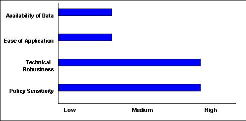
The simplest option for estimating speed (Method 1) is to estimate average speeds by functional class based on speed limits or observed speeds, without consideration of traffic volumes. This approach requires relatively little effort and little or no new data collection. However, it is insensitive to future changes in policy or traffic volumes. This simple method is typically adequate, however, when the area is estimating only direct PM emissions, since the PM exhaust emissions factors in the MOBILE6.2 model do not vary with speed. Note that although this method is more often applied in areas without a TDF model, it can also be applied by locations with a TDF model, particularly if the area is analyzing PM exhaust emissions.
Most regions without a TDF model estimate average speeds by considering traffic volumes and roadway capacities. Three such methods are the HERS model (Method 3), the BPR formula (Method 4), and the TTI method (Method 5). In theory, these methods can be applied to estimate speeds on every individual roadway link, although most regions without a TDF model estimate average speeds by functional class using aggregated volume and capacity information. Some areas use a combination of these approaches, such as a simple method to estimate speeds on lower functional class roadways (i.e., collectors and local roads) and a more complex approach for freeways and arterials.
Speed Estimation
A single average speed is estimated for each facility type, based on the posted speed limit, observed travel speeds, or professional judgment. No analysis of traffic volumes and capacity is used to determine speeds.
Because this method is relatively simplistic, it typically assumes no change in speed over time. Thus, the future year speeds by facility type are assumed to be identical to the base year speeds.
The Colorado DOT assumed an average speed of 35 mph for all arterials and 25 mph for all collectors and local roads in Aspen for estimating PM-10 emissions in a conformity analysis conducted for State Highway 82 (Entrance to Aspen).
The Yuma MPO (Arizona) assumed at average speed of 10 mph for all unpaved roads for estimating PM-10 emissions in its 2003 conformity analysis.
References:
Colorado DOT, "Air Quality Analysis, A Technical Report to the State Highway 82 Entrance to Aspen Environmental Impact Statement," July 7, 1995.
Yuma MPO, "2003 Air Quality Conformity Procedures Outline", draft adopted June 2003.
Lima & Associates "Vehicle Particulate Emissions Analysis" prepared for ADOT, and Yuma MPO, May 2002.
This methodology makes use of the Highway Economic Requirements System (HERS) model to estimate speed. HERS is a computer model developed by FHWA to analyze the effects of alternative funding levels on highway performance. HERS uses HPMS data to analyze the benefits and costs of alternative improvements. HERS computes vehicle speeds for the purpose of determining link travel time and vehicle operating cost, and these speed estimates can be used for calculating emissions. The latest version of the HERS model has a much more accurate speed estimation methodology than the HPMS Analytical Process, which was used by FHWA until the mid-1990s.
The original HERS model was developed for use at national scale. The model can now be customized for use at the statewide level (called HERS-ST). For more information, see FHWA, HERS-ST v20: Highway Economic Requirements System - State Version Technical Report, November 17, 2003.
Available online at http://isddc.dot.gov/OLPFiles/FHWA/010945.pdf.
Speed Estimation
The HERS model is set up and run for the entire state. HERS uses HPMS data as inputs. HPMS data includes only a sample of roadway segments, and the sample size is too small in most cases to produce valid results at the county-level. Thus, the model should be run with the intent of estimating speed by roadway functional class for the entire states.
The latest version of HERS (version 3.54) uses a simplified version of the "Aggregate Probabilistic Limiting Velocity Model" (APLVM) in order to calculate free-flow speeds on each link. The model then applies algorithms to incorporate the effects of grades, traffic-control devices, and congestion on vehicle speed.
For each roadway section, HERS models speed by vehicle type in each direction of travel. Overall average speed per section is aggregated from the speeds of the individual vehicle types. Average link speeds are a by-product of the HERS model rather than one of the standard outputs. Link average speeds are then grouped by the 12 HPMS functional classes (six urban and six rural) for the entire state and averaged by facility type.
Because HERS is designed to evaluate future investment scenarios, it estimates both current and future speeds, based on current and forecasted traffic volumes. If the HERS traffic volume forecasts are consistent with the information used to forecast VMT for emissions purposes (Section 2), then the HERS speed forecasts would be acceptable for emissions estimation purposes. If not, then an alternative method may be needed to estimate future speeds.
Kentucky used this method to estimate statewide average speeds by functional class in rural areas. These values were used to estimate NOx and VOC emissions in two isolated rural areas.
Website: http://transportation.ky.gov/planning/air_quality.asp
Reference:
Bostrom, Rob and Jesse Mayes, "Highway Speed Estimation for MOBILE6 in Kentucky," Kentucky Transportation Cabinet, 2002.
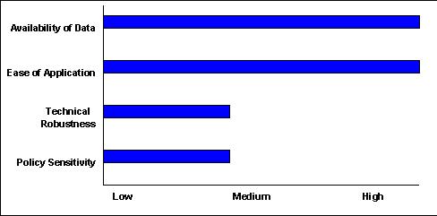
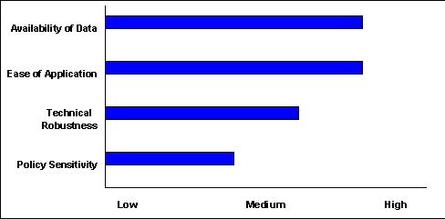
This method can be applied to determine speeds on individual links, which can then be used to estimate a VMT distribution by speed bin for MOBILE6 input. Alternatively, this method can be applied to average VMT and capacity values in order to determine an average speed by functional class.
BPR-type formulas require three inputs: free-flow speed, roadway capacity, and traffic volume. Traffic volume information is developed as described in Section 2 of this report. The accuracy of this method is highly dependent on the accuracy of the capacity and free-flow speed inputs. Procedures for developing these two inputs are described below as well as in the Appendix of this report, followed by procedures for applying the BPR formula.
Free-flow speed estimation
NCHRP Report 387 recommends estimating free-flow speed by link using the following separate equations for unsignalized and signalized facilities.
[Note: additional discussion of free flow speed estimation techniques can be found in the Transportation Research Board's 2000 Highway Capacity Manual.]
Free-flow speed equation for unsignalized facilities:
Free-flow speed = 0.88*Sp + 14
(High-speed facilities have posted speed>50 mph)
Free-flow speed = 0.79*Sp + 12
(Low-speed facilities have posted speed<=50 mph)
where Sp = posted speed limit in mph
Free-flow speed equation for signalized facilities:
![Free Flow Speed = L/[L/S<sub>mb</sub> + N * (D/3600)]](formula15.gif)
where: L = length of facility (in miles)
Smb = mid-block free-flow speed = 0.79*posted speed + 12 mph
N = number of signalized intersections on length, L
D = average delay per signal
D = DF * 0.5 * C(1-g/C)2
where: D = total signal delay per vehicle (sec)
g = effective green time (sec)
C = cycle length (sec)
(Default values for these parameters are provided in the Appendix.)
When using these equations to estimate free-flow speed on a large number of links, it is typically impractical to apply the equations individually for each link. Instead, the equations are used to develop look-up tables of free-flow speeds by facility type and area type. The look-up table is then used to quickly assign free-flow speeds to each link. The Appendix includes an example of such a look-up table.
Free-flow speeds can be determined using other more simplistic methods. Some regions estimate flow speeds by facility type based on the posted speed limit. In other cases, areas add or subtract a fixed amount to/from the speed limit (e.g., speed limit plus 5 mph for highways) or multiply the speed limit by a fixed percentage (e.g., 62% of speed limit for collectors). These simple adjustments to posted speed limits are usually based on a limited sample of measured local speeds that are available for the desired roadway classification. When using these rules for estimating free-flow speeds, the equations often differ based on area type (e.g., CBD, rural, etc.). Other regions estimate free-flow speeds by facility type using observations of off-peak speeds.
Roadway capacity estimation
NCHRP Report 387 recommends a set of equations for estimating capacity that are based on the 1994 Highway Capacity Manual. There are separate equations for freeways, 2-lane unsignalized roads, and signalized arterials.
[Note: a more detailed discussion of capacity estimation techniques can be found in the Transportation Research Board's 2000 Highway Capacity Manual.]
Capacity equation for freeways and unsignalized multilane roads:
Capacity (vph) = Ideal Cap * N * Fhv * PHF
Where: Ideal Cap = ideal capacity in passenger cars per hour per lane (pcphpl)
N = number of through lanes
Fhv = heavy vehicle adjustment factor
PHF = peak-hour factor
Capacity equation for two-lane unsignalized roads:
Capacity (vph) = Ideal Cap * N * Fw * Fhv * PHF * Fdir * Fnopass
Where: Ideal Cap = ideal capacity in pcphpl
N = number of through lanes
Fw =lane width and lateral clearance factor
Fhv = heavy vehicle adjustment factor
PHF = peak-hour factor
Fdir = directional adjustment factor
Fnopass = no-passing zone factor
Capacity equation for signalized arterials:
Capacity (vph) = Ideal Cap * N * Fhv * PHF * Fpark * Fbay * FCBD * g/C * Fc
Where: Ideal Cap = ideal capacity in pcphpl
N = number of through lanes
Fhv = heavy vehicle adjustment factor
PHF = peak-hour factor
Fpark = on-street parking adjustment factor
Fbay = left turn bay adjustment factor
FCBD = central business district adjustment factor
g/C = ratio of effective green time per cycle
Fc = optional user-specified calibration factor
The parameters to use in these equations are provided in the Appendix.
As with free-flow speeds, it is usually impractical to apply the capacity equations individually for every link, so look-up tables are developed.
Computing average speed
The updated BPR formula is as follows:
![s = s<sub>f</sub>/[1 + a(v/c)<sup>b</sup>]](formula12.gif)
where: s = predicted mean speed
sf = free-flow speed
v = volume
c = practical capacity
a = 0.05 for facilities with signals spaced 2 mi apart or less
= 0.20 for all other facilities
b = 10
Many regions have modified the parameters a and b so that the formula calculates speeds that more closely reflect observed local speeds. The original BPR formula uses a = 0.15 and b = 4. Other regions have used values of a as high as 1.0 and values of b as high as 11.
Ohio DOT used the original form of the BPR formula (a = 0.15 and b = 4) to estimate speed in rural areas not covered by a TDF model. To estimate free-flow speeds, Ohio DOT used the upper bound of the table provided in the HCM for each functional class.
Website: http://www.dot.state.oh.us/urban/index.htm
(Speed forecasting procedures described under "documents" section)
References:
Ohio DOT, "Technical Memorandum: Clinton County 2000-2003 STIP/TIP Emissions Estimate," May 25, 1999.
This method can be applied to determine speeds on individual links, which can then be used to estimate a VMT distribution by speed bin for MOBILE6 input. Alternatively, this method can be applied to average VMT and capacity values in order to determine an average speed by functional class. The procedure described below is to determine average speed by functional class.
This method requires estimation of traffic volume, free-flow speed, and roadway capacity, using HPMS data aggregated by area type and functional class.
Volume estimation
HPMS data is first separated into area types and roadway functional classifications. Area type is defined by population - rural (4,999 or less), small urban (5,000 to 49,999), and urban (50,000+). Functional classifications are based on the HPMS classes (Interstate, freeway, other principal arterial, minor arterial, major collector, minor collector, and local).
VMT by area/functional class is allocated into time periods. The four default time periods correspond to the AM peak (7:15 a.m. - 8:15 a.m.), mid-day (8:15 a.m. - 4:45 p.m.), the PM peak (4:45 p.m. - 5:45 p.m.), and overnight (5:45 p.m. - 7:15 a.m.). The default allocation factors for these periods are, respectively, 0.1069, 0.5033, 0.1018, and 0.2880.
VMT by area/functional class and time period is further disaggregated by directional split. The default directional split is 60/40. VMT per time period is divided by centerline miles, yielding volume for each time period, each area type and functional class, and each direction.
Free-flow speed estimation
Free-flow speeds are estimated for each combination of area type and functional class. Default values are shown in the table below. Free-flow speeds are assumed not to vary by time-of-day period or direction.
Default values for free flow speed (mph)
| HPMS Area Type | HPMS Roadway Functional Classification | ||||||
|---|---|---|---|---|---|---|---|
| Interstate | Freeway | Other Principal Arterial | Minor Arterial | Major Collector | Minor Collector | Local | |
| Rural | 70 | 65 | 55 | 50 | 40 | 35 | 30 |
| Small Urban | 70 | 65 | 45 | 40 | 35 | 30 | 30 |
| Urban | 70 | 65 | 40 | 35 | 30 | 30 | 30 |
Roadway capacity estimation
Roadway capacity values are estimated based on the 1994 HCM. For all Interstates, the method uses a default capacity of 2,200 passenger cars per hour per lane (pcphpl). Freeways are assumed to have a default capacity of 2,100 pcphpl.
Other functional class roadways have traffic controls, so capacity is determined using the following equation:
Ci = Si * (gi/C)
Where: Ci = capacity of lane group I (vehicles per hour)
Si = saturation flow rate of lane group i, vehicles per hour of effective green time (vphg)
gi/C = effective green ratio for lane group i
Default values for effective green ratios (gi/C) by HPMS roadway functional class
| Principal Arterial | Minor Arterial | Major Collector | Minor Collector | Local |
|---|---|---|---|---|
0.6 |
0.55 | 0.5 | 0.4 | 0.3 |
Saturation flow rate is calculated using the following equation:
S=fw*fhv*fg*fp*fbb*fa*frt*flt
Where: S = saturation flow rate adjustment factor (rounded to 2 decimal places)
fw = lane width adjustment factor (default is 12-foot lanes)
fhv = heavy vehicle adjustment factor (default is 5%)
fg = approach grade factor (default is 1, level terrain)
fp = parking lane adjustment (none for rural, 1 per hour for urban)
fbb = bus blocking factor (none for rural, 10 per hour for urban, mid-point for small urban areas)
fa = area type adjustment (0.9 for urban area, 1.0 for all other areas)
frt = right turn adjustment factor (shared lane for right turns for all area types, high pedestrians crossing for urban areas, moderate for small urban areas, and low for rural)
flt = left turn adjustment factor (exclusive left turn lanes and protected phasing for rural areas, shared left turn lanes and protected plus permitted phasing for urban areas, mid-point for small urban areas)
If possible, these parameters should be developed using local estimates, for each combination of area type and functional class. Otherwise, the method suggests use of the default values in the table below.
Default saturation flow rate adjustment factors by area type
| Area Type | fw | fhv | fg | fp | fbb | fa | frt | flt |
|---|---|---|---|---|---|---|---|---|
| Rural | 1 | 0.95 | 1 | 1 | 1 | 1 | 0.98 | 0.95 |
| Small Urban | 1 | 0.95 | 1 | 0.98 | 0.98 | 1 | 0.94 | 0.90 |
| Urban | 1 | 0.95 | 1 | 0.95 | 0.96 | 0.90 | 0.90 | 0.85 |
Using the default adjustment factors results in the following default values for hourly lane capacity, by area type and functional class.
Default hourly lane capacities (vehicles per hour per lane)
| PMS Area Type | HPMS Roadway Functional Classification | ||||||
|---|---|---|---|---|---|---|---|
| Interstate | Freeway | Other Principal Arterial | Minor Arterial | Major Collector | Minor Collector | Local | |
| Rural | 2,200 | 2,100 | 1,003 | 920 | 836 | 669 | 502 |
| Small Urban | 2,200 | 2,100 | 878 | 805 | 732 | 585 | 439 |
| Urban | 2,200 | 2,100 | 673 | 617 | 561 | 448 | 336 |
The hourly lane capacity values are then used to estimate aggregate capacity by time-of-day period. To do this, the lane capacities are multiplied by the number of lanes associated with each area type/functional class (lane miles divided by centerline miles). Hourly roadway capacities are then typically multiplied by the number of hours in the time period to produce time period capacities. This procedure is performed for each combination of time period, roadway functional classification, and area type. (Capacity is the same for each direction and time period.)
Computing average speed
Calculation of average speed requires the aggregate volume and capacity as described above and the free-flow speed values. The calculation of speed uses a formula originally developed by the North Central Texas Council of Governments for the Dallas/Fort Worth area. The procedures involves calculating delay using the following equation:
Where: Delay = congestion delay (in minutes/mile);
A & B = volume/delay equation coefficients;
M = maximum minutes of delay per mile; and
V/C = time-of-day directional volume/capacity ratio.
Parameters:
| Facility Category | Parameter | ||
|---|---|---|---|
| A | B | M | |
| Facilities (>3,400 vehicles/hour, e.g. Interstates and Freeways) | 0.015 | 3.5 | 5 |
| Low Capacity Facilities (<3,400 vehicles/hour, e.g. Arterials, Collectors, and Locals) | 0.05 | 3 | 10 |
Congested speeds can then be calculated as follows:
![Congested Speed = 60/[60/Freeflow Speed + Delay]](formula14.gif)
The result is an estimate of average speed for each combination of area type, functional class, and time-of-day period. These values can then be used to determine VMT distributions by speed for the MOBILE6 inputs.
North Carolina used this method to estimate VOC and NOx emissions in donut areas (part of a metropolitan non-attainment area but outside MPO boundaries). North Carolina used this method to estimate average speeds by area type (rural, small urban, urban) and functional class. North Carolina also tested the BPR formula and another speed formula (the Greenshields method), but found that the TTI method produced speed estimates that most closely match observed values.
References:
North Carolina DOT, Davidson County, and the North Carolina Department of Environment, "Emissions Analysis Report for the Transportation Plan for Rural Portion of Davidson County," September 27, 2002.
Rural Conformity Spreadsheet PowerPoint Presentation, Behshad Norowzi, North Carolina Department of Transportation, July 2004.
The use of a TDF model requires development of a computerized roadway network, typically representing all major roadway links in a region. The model then estimates traffic volumes on these represented links, for a base year and forecast years. Thus, areas that use a TDF model have volume and capacity information for all major roadway links, and can use this information to estimate speeds for the purpose of estimating emissions.
This section discusses methods for estimating speeds for links covered by the TDF model, as well as methods for estimating speeds for links outside of the TDF model coverage (i.e., donut areas beyond the MPO modeling area).
A TDF model estimates traffic speed on each link as part of the network assignment process. The assignment process typically determines the route between an origin node and a destination node that results in the shortest travel time. The assignment process is iterative - all trips are first routed based on free-flow travel times, then link travel times are recalculated based on congestion delay, then trips are re-routed based on the new link travel times, and so on until the process reaches equilibrium.
TDF models are typically calibrated so that they closely match observed traffic volumes, but not traffic speeds. Because TDF models must quickly calculate speeds for thousands of links, they use relatively simple equations, such as the BPR formula, and generally do not account for detailed facility or traffic characteristics in the speed calculation. TDF models calculate speeds only for the purposes of facilitating the traffic assignment process, not for the purpose of emissions estimation or other planning practices. Thus, the TDF model speeds may or may not accurately reflect current and future speeds.
Some regions use TDF model speeds directly for developing emission factors (Method 1). Other regions perform adjustments of TDF model speeds to improve accuracy (Method 2), or use a post-processor to estimate speeds rather than use TDF model speeds (Method 3). Use of a post-processor typically relies on methods such as the BPR formula described in Section 3.3.
If the TDF model speeds are determined to be acceptable, link-level speeds can be processed for developing emissions factors in the MOBILE6 model. The best option is to determine the distribution of VMT by speed bin for each facility type. Link volumes are multiplied by link length to calculate link VMT. For each facility type, link VMT is then allocated to speed bins, and the distribution of this VMT become a MOBILE6 input.
Alternatively, links can be grouped by facility type, and an average speed (weighted by VMT) calculated for each facility type. The same process is applied for base year speeds and forecast year speeds.
Butte County, California used this method to develop emission factors for NOx, VOC, and CO. Madera County, California used this method to develop emission factors for NOx, VOC, and PM-10. Both counties used TDF model output to group link VMT by speed for the purposes of estimating a VMT distribution by speed bin.
Bannock County, Idaho used this method to estimate average speeds by facility type for the purposes of developing PM-10 emission factors in MOBILE6.2.
Resources:
Butte County Association of Governments, "Draft Air Quality Conformity Determination for the 2001 Regional Transportation Plan And Adopting Resolution", Adopted April 26, 2001.
Earth Matters, "San Joaquin Valley Air Quality Modeling Procedures - 2001 RTPs and TIPs," 2001.
This method first requires a review of TDF model output speeds to assess their accuracy. Data on observed traffic speeds should be organized by link, and then compared to the modeled speeds on those links. Modeled speeds may be unacceptable for all facility types, or may be unacceptable for only selected facility types (e.g., arterials) or for selected area types (e.g., CBD).
In the case of facility/area types for which model speeds appear accurate, these speeds are used as described in Method 1. The best option is to determine the distribution of VMT by speed bin for each facility type. Alternatively, links can be grouped by facility type, and an average speed (weighted by VMT) calculated for each facility type. The same process is applied for base year speeds and forecast year speeds.
In the case of facility/area types for which model speeds are inaccurate, a variety of approaches can be taken. In some cases, modeled speeds may simply be scaled up or down to better reflect observed speeds. Speeds can also be estimated by applying a formula or look-up table based on the V/C ratio (see Method 3 below). The same process is applied for base year speeds and forecast year speeds.
A variation of this method was used to estimate NOx and VOC emissions in Parkersburg, West Virginia (Wood County). A review of TDF model speeds revealed that the model was overestimating speeds on local roads. For urban local roads, the MOBILE6 local road default speed was used. For rural local roads, an average of the model speed and the MOBILE6 default speed was used.
References:
Wilbur Smith Associates, "Appendix F - Air Quality Conformity Analysis" from the Wood-Washington 20 Year Multimodal Transportation Plan, January 2004.
The method estimates speed using some form of the BPR formula, which is based on the volume/capacity (V/C) ratio and the free-flow speed. BPR-type formulas require three inputs: free-flow speed, roadway capacity, and traffic volume. The accuracy of this method is highly dependent on the accuracy of the capacity and free-flow speed inputs. The development of these inputs is discussed under Method 4 in Section 3.3 and in the Appendix of this report. It also is reviewed below.
Because most TDF models are run for a 24-hour period or for peak and off-peak periods, this method can be used to estimate hourly speeds if this level of detail is desired for MOBILE6 input. To do this, link-level volumes are distributed by hour of day, based on distribution fractions typically developed from local traffic count data. The hourly VMT on each link is calculated by multiplying link volume by link length. Link speeds are estimated based on the
V/C ratio, using the BPR formula, look-up tables, or other methods. A VMT distribution by speed bin then can be calculated for each hour of the day, by facility type.
Free-flow speed estimation
NCHRP Report 387 recommends estimating free-flow speed by link using separate equations for unsignalized and signalized facilities. These equations are presented in the Appendix.
Many regions estimate free-flow speeds based on look-up tables developed from default values in the Highway Capacity Manual, NCHRP Report 387, or other sources.
Some regions estimate free-flow speed by facility type using simplistic methods based on the posted speed limit, such as adding or subtracting a fixed amount to/from the speed limit. For example, one region used the speed limit plus 5 mph for highways based on typical observed speeds. Another region multiplied the speed limit for each functional classification by a fixed percentage (e.g., 62% of speed limit for collectors) developed from observed speeds. When using these rules for estimating free-flow speeds, the equations often differ based on area type (e.g., CBD, rural).
Other regions estimate free-flow speeds by facility type using observed off-peak speeds.
Roadway capacity estimation
NCHRP Report 387 recommends a set of equations for estimating capacity that are based on the 1994 Highway Capacity Manual. There are separate equations for freeways, 2-lane unsignalized roads, and signalized arterials. These equations are presented in the Appendix to this report.
Many regions estimate roadway capacity based on look-up tables developed from default values in the Highway Capacity Manual, NCHRP Report 387, or other sources.
Computing average speed
A variety of equations are used to estimate speeds. The most common is the BPR formula. The updated BPR formula is as follows:
where: s = predicted mean speed
sf= free-flow speed
v = volume
c = practical capacity
a = 0.05 for facilities with signals spaced 2 mi apart or less
= 0.20 for all other facilities
b = 10
Many regions have modified the parameters a and b so that the formula calculates speeds that more closely reflect observed local speeds. The original BPR formula uses a = 0.15 and b = 4. Other regions have used values of a as high as 1.0 and values of b as high as 11.
Ohio DOT uses this method to estimate speeds for small urban areas with TDF models. The TDF model output is used to determine a V/C ratio for each link. Speeds are then estimated using look-up tables taken from the Highway Capacity Manual.
Website: http://www.dot.state.oh.us/urban/index.htm
(Speed forecasting procedures described under "documents" section)
References:
"Technical Memorandum: Clinton County 2000-2003 STIP/TIP Emissions Estimate," Ohio DOT, May 25, 1999.
Statewide Travel Time Study, Gregory T. Giaimo, Ohio DOT, May, 2001.
In metropolitan areas that have a TDF model, there may be "donut" areas that are not covered by the model. These areas often lack detailed information on the roadway network and associated traffic volumes. Therefore, to estimate speeds in these areas, the methods presented in Section 3.3 (areas without a TDF model) can be used. Similar to Section 3.3, average speeds by functional class often must be estimated based on a subset of roadway segments. In some case of donut areas, however, output from a nearby area with a TDF model may be available to provide region-specific speed data to help estimate donut area speeds.
Following are the methods that have been identified in practice to estimate speeds in donut areas not covered by a TDF model, which rely to some extent on data from the TDF model:
In addition, methods the are applicable to areas without a TDF model (see Section 3.3) can also be applied in donut areas, such as use of observed speeds and/or speed limits, or use of a formula and/or lookup tables.
The Kentucky Transportation Cabinet (KYTC) has used this method to estimate emissions in several donut areas. Average speeds by functional class from the TDF model were assumed to apply to the entire nonattainment or maintenance area, including the donut area.
References: M.L. Barrett, R.C. Graves, D.L. Allen, J.G. Pigman, G. Abu-Lebdeh, L. Aultman-Hall, S.T. Bowling, Analysis of Traffic Growth Rates, University of Kentucky Transportation Center, August 2001.
To apply this method, the statewide model is used to determine speeds by link for the donut area. The metropolitan area TDF model is used to determine speeds by link for the modeled areas within the same county (i.e., for the links contained within both TDF models, speeds are based on the metropolitan area TDF model). Speeds from the two models are then combined, weighted by VMT, and averaged by functional class. The resulting average speeds by functional class are used for the entire county (both modeled and non-modeled areas).
Local roads are not covered by statewide models. To estimate speeds for local roads in the donut area, an average local road speed is calculated for the area covered by the TDF model.
Michigan Department of Transportation (DOT) applied this method to estimate emissions in Allegan County. Michigan DOT maintains a statewide TDF model that includes 2,300 zones and a subset of roadway links. The MPO TDF model covers portions of Allegan County (City of Holland and three townships).
References:
Michigan DOT. "Allegan County Air Quality Conformity." Undated.
Michigan DOT, Travel Demand Analysis Section. "Technical Documentation of the Procedures Used to Develop VMT and Speed Estimates for Michigan Non-Attainment Counties Containing a Modeled Urban Area." 1995.
[11] Technical Guidance on the Use of MOBILE6.2 for Emission Inventory Preparation, U.S. EPA, August 2004.
[12] Technical Guidance on the Use of MOBILE6.2 for Emission Inventory Preparation, U.S. EPA, August 2004.
[13] This paragraph adapted from Guidance for the Development of Facility Type VMT and Speed Distributions, U.S. EPA, Report Number M6.SPD.004, February 1999.
[14] Additional detail on BPR formulas and related methods can be found in the Transportation Research Board's 2000 Highway Capacity Manual.

