This section describes in greater detail those research topic areas considered high-priority. Each recommendation is described in order of its rating by participants of the one-day workshop. A brief description of the goals of that research, value to the transportation community, background, and example projects are provided. Four research topics were considered high priorities as shown in Table 3. These research priorities are summarized in Table 6.
Table 6. High priority research issues.
| Research issue | Monitoring | Characterization | Emissions | Modeling | Controls | Recommendation number from Literature Assessment (Tamura et al., 2005). Also available in Table 1 in this document. |
|---|---|---|---|---|---|---|
| H.1. Monitor near roadways | X | LA-1 | ||||
| H.2. Evaluate hot-spot models | X | LA-16 | ||||
| H.3. Develop and evaluate PM emissions models | X | LA-14 | ||||
| H.4. Evaluate control strategy programs | X | LA-19 |
Research goals. Provide near-roadway monitoring and traffic data needed to evaluate hot-spot modeling tools, determine concentration gradients of PM and precursors near roadways, and support health effects research. Figure 4 illustrates a mobile monitoring unit used by the UCLA-based Southern California Particle Center to monitor near-roadway PM concentrations.
Figure 4. Mobile particle instrumentation unit from the UCLA-based Southern California Particle Center Supersite. Photo courtesy of the Southern California Particle Center Supersite.
Value to Transportation Community. The EPA has proposed conformity regulations that could require MPOs and DOTs to estimate the impacts of transportation projects near roadways (i.e., "hot-spot or localized" problems). However, available modeling tools to meet these proposed requirements have not been evaluated against PM monitoring data (see Section 3.2). Data to perform these hot-spot model evaluations are not available from current PM monitoring networks, because these networks are not designed to characterize near-roadway PM or PM precursor concentrations. Near-roadway monitoring of PM and traffic is needed to provide data to evaluate the modeling tools and ensure that they accurately predict PM concentrations. Near‑roadway monitoring data can also be used to
Background. A growing body of literature shows that morbidity, mortality, and cardiopulmonary outcomes are a function of inverse distance to major roadways, traffic density, and type of traffic (i.e., gasoline/diesel vehicle split). For example, epidemiological studies have linked exposure to traffic with asthma, stroke mortality, and decreased life expectancy (Wjst et al., 1993; Nicolai et al., 2003; Duki et al., 2003; Hoek et al., 2002a; Roemer and van Wijnen, 2001b) . However, there are no definitive studies identifying which pollutants (i.e., gases, particles, ultrafine particles, or mixtures of pollutants, etc.) are responsible for the health effects.
Monitoring studies have shown only slightly elevated concentrations of PM mass near and on roadways (Roemer and van Wijnen, 2001a; Hoek et al., 2002b; Tiitta et al., 2002; Wu et al., 2003; Harrison et al., 2003; Etyemezian et al., 2003; Weijers et al., 2004; Zhu et al., 2002b; Zhu et al., 2002a). Near-roadway concentrations of black carbon, CO, and particle number are more elevated. (e.g., Sardar et al., 2004; Fine et al., 2004; Zhu et al., 2002b; Zhu et al., 2002a) .
Example Projects. In designing "near-roadway" monitoring projects, the following objectives should be considered:
Multiple monitors will be necessary to characterize PM concentration gradients. Use of a mobile platform with real-time particulate monitors may also be valuable in characterizing such gradients. Not all research goals can be met with a single sampler at one location.
Multiple samplers may be necessary at each monitor to characterize different chemical components of PM and its precursors. Chemically speciated PM monitoring data would be helpful for identifying the relative amounts of exhaust PM and fugitive PM (i.e., resuspended road dust, brake wear, and tire wear).
Measurements of size distributions are needed to characterize spatial gradients for PM10, PM2.5, and ultrafine particles to support model development and evaluation.
Chemical speciation of PM components for various size ranges should be considered as well, since the toxicity may be determined by a combination of chemical and physical factors.
It may be more cost effective to leverage near-roadway studies to include measurement of several pollutants of interest, such as mobile source air toxics, tracer compounds to detect diesel emissions, carbon monoxide (CO), black carbon, and ultrafine particles.
Collecting traffic data will aid transportation and air quality personnel in evaluating the impacts of congestion mitigation on tailpipe and fugitive PM emissions (see Sections 4.1 and 4.6).
For example, a near-roadway monitoring study could be designed to evaluate the effects of congestion mitigation and control strategies on vehicle emissions. Monitoring concentrations of PM and its precursors near a specific roadway before and after control strategy implementation may allow quantitative evaluation of control strategy efficacy. Data from this type of study could be used to evaluate air quality impacts on a number of pollutants (e.g., PM, PM precursors, air toxics, or ozone precursors) to identify benefits for a range of air quality problems.
Research goals. Evaluate hot-spot (i.e., localized) models for their ability to predict PM concentration gradients near roadway intersections and free-flowing roadways. Figure 5 illustrates hot-spot modeling results based on the CAL3QHC model.
Figure 5. Predicted downwind pollutant concentrations as a function of wind speed and distance from the roadway from the EPA's CAL3QHC model, not including background concentrations. Reprinted from Tamura and Eisinger (2003) .
Value to Transportation Community. The EPA has proposed conformity regulations that could require MPOs and DOTs to estimate the impacts of transportation projects near roadways (i.e., "hot-spot or localized" problems). However, available modeling tools used to meet these proposed requirements have not been evaluated against PM monitoring data. It is well established that PM concentrations can be higher in the vicinity of roadways (see Section 3.1). MPOs and DOTs will need modeling tools that accurately predict PM concentrations at monitors near roadways as a function of distance, and will need to understand what factors significantly influence the model results.
Background. Hot-spot modeling tools are vital for completing environmental impact reports and project-level analyses. During the one-day workshop, members of the transportation planning community expressed concern that existing modeling tools may be incapable of accurately assessing PM hot-spot problems; they rated this concern as a high-priority.
Historically, hot-spot modeling (and the associated conformity regulations) has focused primarily on CO, which is inert on these spatial scales. Models used for this purpose have incorporated the effects of dispersion due to dilution and air movement, but do not assume any chemical or physical processes take place. In contrast with CO, PM formation and settling processes are not necessarily negligible and fugitive PM may need to be treated separately from exhaust PM (see Figure 6).
Figure 6. Attenuation of PM10 and PM2.5 mass concentrations with time and vertical mixing volume. (Reprinted from Countess et al., 2001 with permission.)
EPA regulations for CO hot-spot analyses recommend the use of continuous line-source dispersion models, such as the CALINE model for free-flow roadways and the CALINE-based CAL3QHC model for incorporating queuing at intersections. However, these models perform poorly when the wind is nearly parallel to the roadway (Benson, 1992) . The recently developed ROADWAY-2 and HYROAD models showed agreement with measured pollutant concentrations for multiple wind directions (Rao, 2002; Carr et al., 2002b).
Example Projects. Evaluation of localized turbulence and dispersion models has been performed in the past (e.g., Rao, 2002) . However, these evaluations have been for inert gas-phase pollutants. Localized concentration gradients of PM need to be evaluated in the same way as in Rao (2002) to determine if deposition and chemical transformation are important. If so, these factors need to be added to the current hot-spot models.
Research goals. Develop and evaluate PM emissions models that predict the effect of roadway projects on PM and PM precursor emissions. Figure 7 reproduces graphics from an FHWA report that illustrate the deficiency of MOBILE6.2 model runs to predict PM emissions variability with speed changes.
Figure 7. PM emissions as a function of speed from the MOBILE6.2 emissions model. Figure reprinted with permission from Granell et al., (2004) .
Value to Transportation Community. Currently, all MPOs and DOTs (except those in California) are required to use the EPA's MOBILE emissions model to calculate emissions budgets to fulfill conformity requirements. For MPO and DOT users, there are two applications of PM emissions models important for transportation conformity assessments: project-level and regional analyses. To complete project-level analysis, emissions are needed for a specific roadway that may be dependent on specific operating modes, and may require sub-hourly output information. Ideally, emissions models for these projects would take into account details such as acceleration (e.g., on-ramp design), grade, and traffic signals. Regional emissions analyses typically focus on assessing average speed and traffic volume information for specific time periods (e.g., morning and afternoon peak periods, and off-peak periods). Regional analyses may need to consider the impact of control measures for conformity, and therefore require the ability to model the effects of available control strategies.
Background. Emissions modeling tools are vital to MPOs and DOTs for completing regional and project-level analyses. During the one-day research workshop, members of the transportation planning community expressed concern that the existing version of the MOBILE model does not include needed emission factor resolution to accurately estimate on-road PM emissions. For example, concern was expressed regarding the lack of speed-corrected heavy-duty diesel vehicle (HDDV) PM emissions. Because HDDV emissions are thought to contribute a large fraction of transportation-related PM, omitting speed correction factors may result in inaccurate model emissions. Transportation planning community participants considered this problem to be a high priority.
The NRC recommended the EPA assess and identify the levels of accuracy needed for the different mobile source emission model applications (National Research Council, 2000); this task has not yet been completed. Without evaluation of the accuracy needs for emissions model applications, it is not clear if the emissions budgets used to develop SIPs and future emissions budgets are realistic or achievable.
MOBILE calculates emission factors based on ambient temperature, vehicle types, average speed, and other variables. There are several known deficiencies with the MOBILE model:
In response to recommendations to improve mobile source modeling, the EPA is devoting its resources to developing a new emissions model, named "MOVES", to replace MOBILE, although it is not expected to be available for the PM2.5 SIPs due in 2008 (Koupal, 2005). Notwithstanding the development of the MOVES model, MOBILE will be used to prepare the next round of 8-hr ozone and PM2.5 SIPs, and will therefore be used to establish 8-hr ozone and PM2.5 conformity emission budgets. Thus, the transportation community has a longer-term vested interest in correcting known MOBILE model deficiencies.
The MOVES model will address some of the deficiencies in MOBILE by characterizing vehicle activity using vehicle specific power (VSP) rather than average speed. MOVES model development is being evaluated by CRC Project E-68, but it is likely that the transportation community will desire additional evaluations that are specific to highway projects and conformity applications (Lindhjem et al., 2004) .
Example Projects. For the development and evaluation of emissions models, example projects could include
Research goals. Identify and evaluate control measures with incomplete information on costs, benefits, or other knowledge gaps for PM and other air pollutants. Figure 8 illustrates example control measure situations.


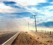
Figure 8. Collage of control measure situations. High occupancy vehicle lanes in Denver (left-courtesy of The Regional Transit District-Denver, CO), bike lane in San Francisco (center-stock photo courtesy of San Francisco Metropolitan Transportation Commission), and fugitive dust in Nevada (right-photo courtesy of Business Environmental Program of Nevada).
Value to Transportation Community. Transportation planners often work with their air quality agency partners to adopt and implement control measures to reduce mobile source emissions. Choosing the appropriate control strategy for a region requires knowledge of the costs and benefits of each measure. This research topic will identify and evaluate control measures with incomplete or missing cost and benefit information to provide policymakers with the necessary details to make informed policy choices. This research topic at least partially depends on the compilation of control strategies (see Section 4.2) and would benefit from an up‑to-date on-line repository (see Section 4.4).
Background. Control measures come in many different forms and can have varying efficacy and costs. Control measures can be grouped into at least six different areas:
Comparisons of cost-effectiveness evaluations for air pollution controls vary across orders of magnitude (Wang, 2004; Wang, 1997; Transportation Research Board, 2002) . A large amount of the variability in these evaluations was due to differences in evaluation methodologies, which are often not specified or incorrectly applied (Cambridge Systematics, 2001). Since cost methodology guidance is not available for mobile source control strategies, different approaches have been taken. For example, some cost methodologies are based on costs to consumers, while others are based on costs to manufacturers. Implementation costs are often excluded, particularly with respect to those incurred by regulatory agencies (i.e., regulatory development and enforcement). In addition, some measures, such as emissions abatement devices, may be less effective at the local or regional level because of interstate and inter-regional travel.
Example Projects. One possible project would be to identify popular ozone control strategies that reduce VOC or nitrogen oxide (NOx) emissions with incomplete cost-effectiveness information for PM. These could then be analyzed for their efficacy for reducing PM and PM precursors as well.
A specific control measure evaluation could be to further investigate the efficacy of operating street sweepers. Some studies have questioned whether sweepers are beneficial (e.g., Etyemezian et al., 2005).
Analyses should provide sufficient information to assess the costs and benefits of each control strategy for PM and precursors, as well as for other pollutants like ozone precursors and mobile source air toxics where applicable.