• Air Toxics
• CMAQ
• Conformity
• It All Adds Up

• Laws and Regulations
• Maps
• Policy and Guidance
• Research
  • General Practice
  • Air Quality Planning and SIPs
  • Emissions Analysis
  • Land Use
  • Multi-Jurisdictional (Complex) Areas
  • Project Level Conformity
  • Small Urban and Rural Areas
  • Tools & Methodologies
  • Transportation Control Measures
• Resources
• Models & Methodologies
• Training
• Air Quality Newsletter

Project Level Analyses

Chapter 4. Port Analysis

One of the objectives of this study was to develop transportation data representative of the activity taking place at port and intermodal facilities that can be used to improve project-level emission estimates for like facilities in MOVES model applications. Vehicle activity at port and intermodal facilities have a unique combination of characteristics that is important to account for in an emissions analysis. This chapter presents information on travel-related data from three sample ports that can be used, in combination with the port specific VSP profiles discussed in Chapter II, to improve the quality of an emissions analysis by including inputs to represent these data in MOVES. Chapter VI provides a demonstration of how these data could then be applied in a MOVES emissions analysis for another port, in this case, the ports under the control of the Port Authority of New York and New Jersey.

A. PORT ANALYSIS

A number of U.S. ports were surveyed for information about the truck travel patterns in and around those ports, with the objective of identifying ports that could serve as examples of expected travel patterns at other U.S. ports. This review identified three ports that the consulting team felt were able to provide recent, relevant data for others to use. These three ports were: Everglades, Florida; Savannah, Georgia; and Long Beach, California. This sample of ports provides information for a Gulf of Mexico port, an eastern seaboard port, and a west coast port.

The port analysis is a separate phase of the study and is not directly connected to the microsimulations described previously. The travel patterns identified in this chapter can serve as guidance to planners doing port analyses when no local data are available.

1. Summary of Port Statistics for Three Selected Ports⁸

Table IV-1 summarizes key data from the three selected example ports for 2009. This data is provided so that analysts can compare the characteristics of their port with those that have been evaluated for this FHWA-sponsored study. These data provide a sense of scale on the activity present at each port.

^* Twenty-foot Equivalent Units.
^**Georgia Ports Authority's total: Port of Savannah and Port of Brunswick.
^***Includes direct jobs only. Does not include induced, indirect, nor related user jobs.

2. Development of Truck Trip Distributions

a.         Trip Length Distribution To/From Port Facilities

To study the distance of trips to and from port facilities, three previous port gate surveys were used. The following describes each of the surveys:

Everglades:  Port Everglades conducted a gate survey from June 21st to June 23rd of 2008. This survey captured a total of 121 trucks at the port's terminals.
Savannah:  The Port of Savannah conducted a gate survey on July 18th and July 19th in 2006. This survey captured a total of 887 trucks at the port's terminals.
LA/Long Beach: The Port of Long Beach conducted a gate survey in January of 2005. This survey captured a total of 2,723 trucks at the port's terminals. This is by far the highest volume of trucks surveyed of all of the locations analyzed in this report.

While each of the surveys asked a variety of different questions, the question that they all have in common is the last stop and next stop of the truck entering or leaving the port. This data was used to geocode the locations of these stops. Depending on the level of detail given in the response, one of several geocoding methods was used, which includes address matching, center of city, and center of state. The LA/Long Beach survey and the Savannah survey had many addresses available, especially for local trips. The Everglades survey was done completely by center of city. Center of state was only used in a few circumstances for long distance trips where no other information was available. Next, the route distance between these locations and the port were measured using routing software in TransCAD and the National Highway Planning Network (NHPN). It should be noted that these distances represent the actual driving distance of the truck on particular roadways, not the straight line distance between two points.

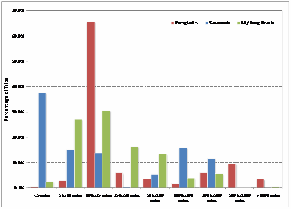
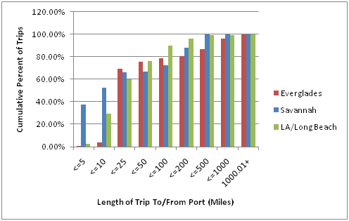
Figure IV-1 shows a graphical representation of the number of trips and their distance to/from the port for Everglades, Savannah, and LA/Long Beach, respectively. The distances were summarized into ranges. Figure IV-1 and Table IV-2 show the percentage of trips for each port that fall into various short distance and long distance ranges. Figure IV-2 and Table IV-3 show the same ranges, but with the cumulative percent of trips under certain thresholds. The results show that the trip distances vary greatly among the three ports studies, likely due to the different geography of cities around the ports. However, a general observation can be made that in all cases a large majority of trips (80-96 percent) are under 200 miles. This is an important distinction for air quality planning using the MOVES model because trucks traveling greater than 200 miles are considered long-haul and trucks traveling less than 200 miles are considered short-haul in MOVES.

Figure IV-1. Percent of Port Terminal Truck Trips at Certain Distance Ranges

Figure IV-2. Cumulative Percent of Trips at Certain Distance Ranges

b.Truck Type Distributions

During the port gate surveys, information was also collected about the type of truck. While many of the surveys included detailed body types, such as container or flatbed, it is only important to differentiate between single unit trucks and combination trucks for the purpose of emissions modeling using MOVES.⁹ In MOVES modeling, both single unit and combination trucks are further distinguished as either short haul or long haul trucks. Each of these different truck categories is assigned different driving cycles in MOVES, leading to differing emission factors for each truck category. Table IV-4 presents these summarized results, which shows almost all combination trucks for all three ports.

c. Road Type Distributions for Trips To/From Port Facilities

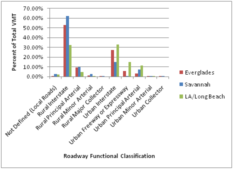
During the routing of the trips to and from ports in the TransCAD software, information was kept on the functional classification of roadways taken. This functional classification information is available for each link in the network on the NHPN, which was used in the TransCAD analysis. The total VMT on each functional classification of roadways for all trips associated with each port was output by the software.

Figure IV-3 and Table IV-5 show the percent of VMT for all trips to and from each port that are spent on each roadway functional classification. It should be noted that the not defined category includes links in the NHPN that have no roadway classification and centroid connectors created by TransCAD to connect the origins/destination with the NHPN roadway network. In both cases, these represent local roads because the NHPN contains the higher classified roadways.

Figure IV-3. Percent of Total VMT by Roadway Functional Classification for the Port Terminals

The TransCAD software is programmed to choose a route that takes the highest roadway classification for the longest period possible, much as a truck driver would choose such a route to minimize the total driving time. Therefore, it follows that interstates and urban freeways/expressways are the most traveled for trips from all three ports. In general, the percent of VMT spent on lower classified roads goes down with the lower roadway classifications. For example, principal arterials are generally the second most traveled and minor arterials are generally the third most traveled. Due to the availability of certain roadway types around each port and the rural/urban geography, the exact percentages from each port vary substantially. For example, Savannah has the highest percentage of VMT on rural interstates because the Savannah urban area is relatively small and Georgia in general has fewer urbanized areas than Florida or Southern California.

This VMT distribution by roadway functional classification is important to emissions modeling because it provides some indication of the speed that trucks drive traveling to and from ports. The speed is correlated with a particular emission rate, which is used to calculate total emissions. For example, rural interstates could be assumed to have a speed of 65 mph for which a particular emission rate could be looked up. For Savannah, that emission rate would be multiplied by 61.95 percent of the total VMT for the port to find the total emissions on rural interstates. A similar process would be followed for the other functional classifications, and emissions for all roadway functional classes would be summed to find the total emissions for trips to and from the port.

d. Time of Day Distributions for Trips To/From Port Facilities

No readily available information was found on the distribution of truck trips by time of day for the three ports analyzed. A reasonable assumption to make in the absence of survey data on time of day distributions is that the number of truck trips associated with the port terminal is relatively flat during the course of the port's normal operating hours.

e. Truck Age Distributions

No readily available information was found on the distribution of the age or model year of the trucks serving the three ports included in this port analysis. However, data on the age distribution of trucks serving the Port Authority of New York and New Jersey ports (the ports used for the emissions demonstration in Chapter VI) were available. That information is shown here since this is the sample port used to demonstrate the application of this port analysis in estimating port emissions. The truck age distribution for these New York/New Jersey ports was created based on data in "The Port Authority of New York and New Jersey Drayage Truck Characterization Survey at the Port Authority and the Global Marine Terminals."  The purpose of that survey was to collect information on the age of drayage trucks in six terminals within the Port Authority of New York and New Jersey. Figure IV-4, which was used to develop the truck age distribution, illustrates the percentage of trucks of each model year.

Figure IV-4. Model Year Distribution of Trucks Visiting the Port Authority Terminals and Global Marine Terminal

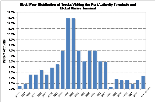
The Port Authority of New York and New Jersey Drayage Truck Characterization Survey at the Port Authority and the Global Marine Terminal, December 2008, Page 3.

The trucks surveyed were categorized as being owner-operated or owned by other than the driver. It is important to note that for the Port Authority of New York and New Jersey, the percentage of owner-operated trucks in each model year made up approximately two-thirds of the sampled trucks. The survey results also indicated that a large percentage of trucks newer than 2003 are not owner-operated trucks, but rather, are fleet vehicles. Therefore, when analyzing emissions from ports with a relatively high proportion of fleet vehicles serving the port, the age distribution should be shifted to include a larger percentage of newer trucks.

Table IV-6 presents the MOVES age distribution input that was developed from the above data to perform calendar year 2008 emission modeling. The age fractions were selected as follows:

• Age ID 0:  model year 2008 in the figure above (the newest model year fraction; this is 2008 in the MOVES input as this is the year being modeled) ~ 0.5 percent;
• Age ID 1:  model year 2007 in the figure above ~ 0.95 percent; etc.;
• Age ID 22:  model year 1986 in the figure above ~ 1.6 percent; and
• AgeID 23 through 30: the remaining fraction was evenly distributed between older trucks (the sum of the age fractions in the MOVES input file must be 1).

B. ESTIMATING TRUCK TRIPS GENERATED AT INTERMODAL FACILITIES

For existing port facilities, the number of truck trips can be estimated using gate count data, if available, or conducting a manual count of trucks entering the facility over a specified period of time. For new or expanded port and intermodal facilities, estimates can be made based on estimates of the facility acreage or expected ship or rail car arrivals. A training session provided by FHWA entitled "Multimodal Freight Forecasting in Transportation Planning: Session 10, Facility and Site Planning Needs and Applications" related truck trips per day to total acreage, ship arrivals, and rail cars per year using Philadelphia, Pennsylvania data. The results for this are shown below.

All Facilities:  Truck trips/day = 3.08 x Total Acreage
Ports: Truck trips/day = 1.90 x Ship Arrivals/year
Rail: Truck trips/day = (1.87 x Acreage) + (0.00517 x Rail Cars/year)

C. POTENTIAL APPLICATION

The information and methodology presented above can provide ideas for how to derive some of the inputs necessary for an emissions analysis of truck trips to and from a port facility. This data could be considered if no local data is available. Averages from all three ports tend to be more reasonable when the categories are aggregated more as shown below.

Total VMT To calculate total VMT generated by trucks traveling to and from a port, the total volume of trucks can be distributed into length of trip bins shown in Table IV-7 using the average column. Then these volumes can be multiplied by the appropriate distance for each bin located in the last column of Table IV-7. If the port of interest is known to be in the same area of the country as one of the three ports shown, or known to be in a geographic area with similar characteristics to one of the three ports shown, in terms of the distance to likely origins and destinations, the distribution can be adjusted to be closer to or equal to the distribution for that port.

Road Type Distribution As one of its inputs, MOVES requires a distribution of VMT among roadway types, which it defines as restricted and unrestricted access roadways in rural and urban areas. The percent distributions by FHWA functional classification presented above were grouped into these four MOVES roadway types as shown in Table IV-8. The averages may be used as a default, or the values from one of the three ports may be used if the area around the port of interest is known to be similar in terms of urban/rural split. It should be noted that the subtotals in the table show that while different ports have different urban/rural splits, the split between restricted and unrestricted access is similar among all three ports.

Vehicle Type Distribution MOVES requires VMT distributed by vehicle type as one of its inputs. While it is possible that single unit trucks could serve ports, Table IV-4 above shows that 97-100 percent of trucks traveling to and from ports are combination trucks. For this study, it can be assumed that all trucks are combination trucks. MOVES also defines trucks by short haul and long haul, which is defined respectively as trips below and above 200 miles. As shown in Table IV-5, on average 13 percent of trips are long haul and 87 percent of trips are short haul. Therefore, for this study, 0 percent single-unit short haul trucks, 0 percent single-unit long haul trucks, 87 percent combination short-haul trucks, and 13 percent combination long-haul trucks were used.