
FHWA-HEP-20-010
This guide introduces some of the basic concepts in highway-related noise modeling by using TNM 3.0. It includes detailed steps to create a basic project with two roadways, two receivers, a building row and one perturbable barrier.
This guide will walk you through the steps to:
Note that this walkthrough is not an exhaustive review of all functionality. To increase accessibility, this walkthrough does not utilize any tools that require an ESRI runtime license. Additional details can be found by searching appropriate areas of the Help Menu inside TNM 3.0.
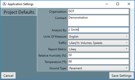
To start, we want to set some default settings that each project will start with. After launching TNM 3.0, go to the Settings tab and select Application Settings to set default settings. This will open a new dialog where project defaults can be entered. Details on each of these interfaces can be found in the Help Menu by searching for the particular item. Enter appropriate information for each field. Click the Save Settings button to save these default settings. The figure below shows example default inputs.
With these default settings in place, we can create a new project that will inherit these settings. Click on the left-most tab (the tab showing a globe icon of the "world"). Select New Project to open a new input window. The New Project dialog box will open. This window allows you to set some information about your new project. The first three fields, Organization, Contract and Analysis By, allow entry of general data about the project. The next field, Type, allows you to select between three options: Cartesian, Geographic and Projected. You should use Cartesian when the input coordinate data are in orthogonal coordinates without any reference to a particular projection. This will enable options in the Project Settings fields (Category, System and Units) that are appropriate for studies in either English or Metric units without projection data. You should use Geographic or Projected when your data are in spherical coordinates, e.g. latitude, longitude and elevation (for Geographic) or derived from projections that are designed to minimize map deformations near a particular location (for Projected). Details on each of these interfaces can be found in the Help Menu by searching for the particular item. For this example, enter the options shown in the figure below and then press the Create button.
![Screenshot showing the 'New Project' dialog box and sample inputs. The inputs are as follows: Organization is 'DOT'; Contract is 'Demonstration'; Analysis By is 'J. Smith'; Type is 'Projected'; Category is 'StatePlanNad1983Feet'; System is 'NA1983StatePlanVirginiaNorthFIPS4501Feet'; Units are 'Foot_US'; Traffic is 'LAeq1h: Volumes, Speeds'; Report Metric is 'LAeq'; Relative Humidity (%) is '50'; Temperature (degrees F) is '68'; Ground Type is 'Hard Soil'; LOS Distance Limit [ft] is '500'; Name is 'Demonstration_Project'; and Description is 'This project demonstrates the steps involved in using TNM 3.0 for a simple study.'](tnmv3_images/getting_started_f2.png)
After the Create button is pressed, the default Project View will be opened. See the figure below. There are five main areas in the application when it opens in its default view: 1) TNM Toolbar, 2) Edit Pane (Edit and Search tabs), 3) View Pane (Plan View, 3D View, Section View and Report View tabs), 4) Legend Pane, and 5) Object Details Pane. We will show some example uses of each these next. Further details on each of these can be found in the help menu by searching for the particular item.
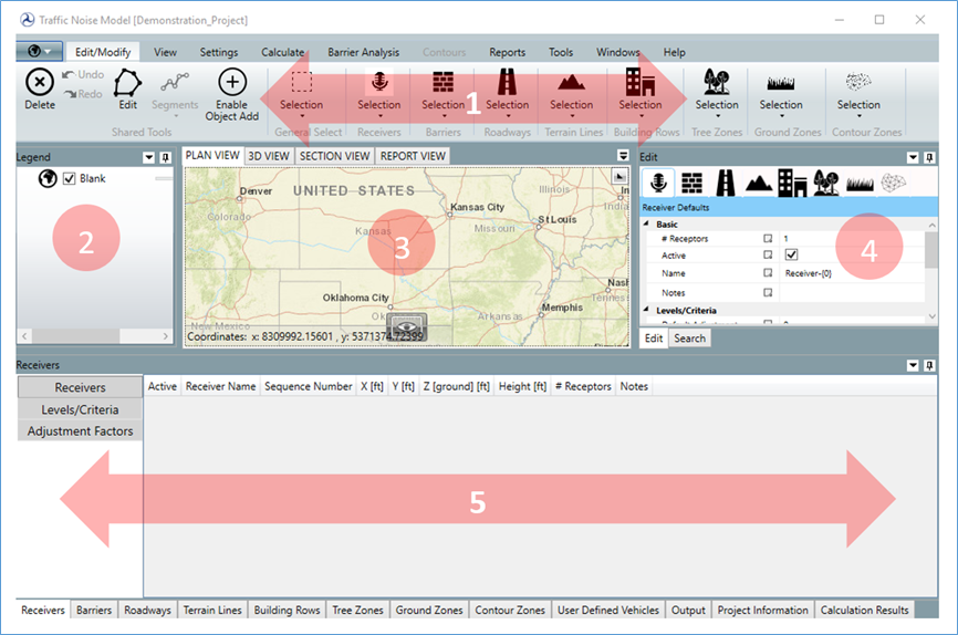
(The TNM Toolbar is found at the top of the application and is used to perform various functions in TNM. You can minimize or maximize the toolbar by right clicking and selecting Minimize the Ribbon. TNM Toolbar details can be found in the Help Menu under TNM Toolbar.)
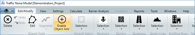
To start adding TNM objects to the project, go to Edit/Modify in the TNM Toolbar and click on the Enable Object Add button.
(The Edit Pane is found on the right side of the application below the TNM Toolbar and contains information about object defaults that are used when creating new objects and allows you to select an object type to add to the project. Edit Pane details can be found in the help menu under Edit Pane.)
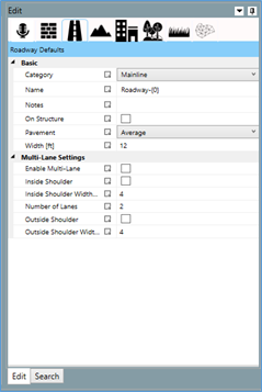
In order to tell TNM that you wish to add a roadway to the project, select the Roadway button at the top of the Edit Pane. When selected, it will be outlined in blue as shown in the figure below. For the time being, leave the default values alone. These can be changed later when you want to add additional roadways.
(The View Pane displays the map and associated map data using different visualization methods. The View Pane is comprised of the following four sub-panes used to represent project data in various visualization forms: Plan View, 3D View, Section View, and Report View. View Pane details can be found in the Help Menu under View Pane.)
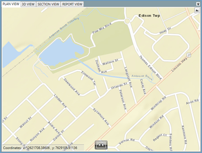
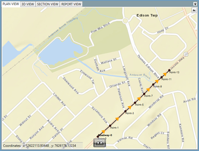
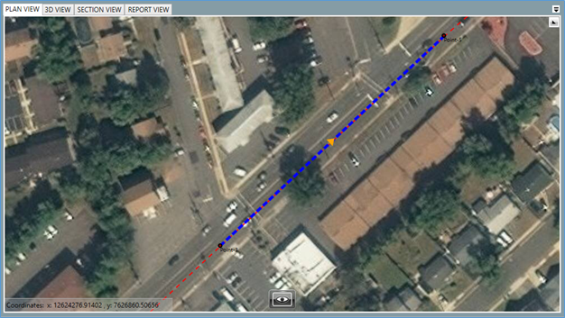
Having already pressed Enable Object Add under Edit/Modify in the TNM Toolbar and having already selected the Roadway button in the Edit Pane, add a roadway to the project by clicking the left mouse button several times in the Plan View sub-pane of the View pane at several points along a displayed roadway as shown in the figures below, here moving south west to north east. Double click to stop creating new points for this roadway object.
Note, one can move around in the Plan View by clicking on the left mouse button while hovering over an area of the map that does not have any TNM objects and then moving the mouse, e.g. left to right or up and down. One can zoom in or out in the Plan View, making it easier to see object details or easier to see large areas of the map by scrolling with the scroll wheel on the mouse. One can also change the type of map displayed by hovering the mouse over the "eye" icon in the center southern area of the Plan View. For example, after pan and zooming and selecting the aerial view, the map now looks like that shown in the next figure.
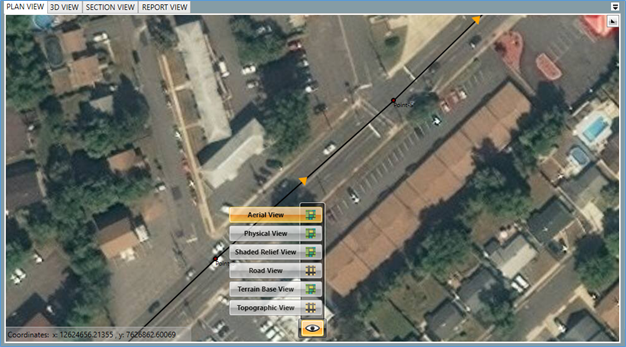
This aerial view shows that the placement of the road is not quite right. While it is generally more accurate to obtain coordinates for TNM objects from state or municipal plans, this exercise provides an opportunity to see how some of TNM's editing features work.
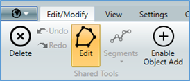
Go back to the Edit/Modify toolbar and select the Edit icon. (See below.) Once this is selected, TNM objects can be edited graphically by selecting points, segments or entire objects. (Edits can also be made in the Object Details Pane regardless of whether the Edit icon in the toolbar is selected. We will discuss this later.)
We want this roadway to be in the center of the two lanes traveling northeast, therefore we need to move each point. Do this by holding the left mouse button down while hovering over a roadway start or endpoint (when hovering over the point it will change color from dark red to light blue). While holding the left mouse button down, drag the mouse so that the roadway point is moved to the desired location in the Plan View. It is easiest to do this by zooming in close to the point, moving it by selecting the point and dragging with the mouse, then panning the map, as discussed previously, to the next point. The next figure shows the roadway, now shifted to align with the center of one lane of traffic. (Note, that a dashed red line is used to show that an object is selected. A dashed blue line shows which segment is selected. To unselect an object, double click on an empty area of the map.)
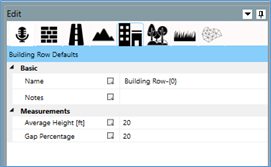
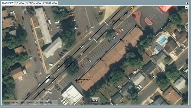
Now we want to add the other objects in this project, that is, a second roadway, two receivers a building row and one perturbable barrier. Follow the same procedure as adding the first roadway for the second, but this time start clicking on points in the map in the northeast and continue down to the southwest to get the direction of the roadway correct. Once it is roughed in, zoom in to make fine adjustments to the roadway location. Next, in the Edit pane, select the Building Row icon (see figure below), and then follow a similar sequence of left mouse clicking in the Plan View to create a building row in the project.
At this point your Plan View should look something like the figure below.
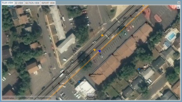
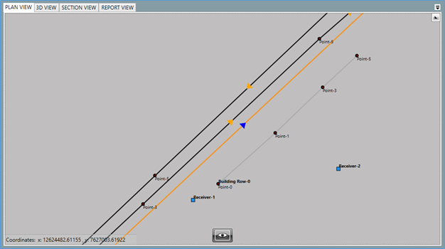
Next add two receivers following a similar approach. Place one near the roadway and one on the opposite side of the building row. Finally add a barrier between the near roadway and the receivers. Once finished, your project should look something like the figure below.
(The Legend Pane displays the layers and/or features that have been added to a project map. When you apply a feature to the map, such as a roadway, it will be listed in the Legend Pane. Once a feature is listed in the Legend Pane, you can choose whether to have that feature viewable on the map and you can increase or decrease its transparency. Legend Pane details can be found in the Help Menu under Legend Pane.)
At this point, it may be easier to simplify the view so that we can see the objects more clearly. We can change the map type by hovering over the "eye" icon and selecting a different map; however, the cleanest look can be obtained by going to the Legend pane and unchecking the "world" icon. This will hide the map entirely so that the project now looks like the figure below.
We have the x- and y-coordinates for the objects that we want in our project, but we do not have z-coordinates or other parameters that important to the run. We can add these by going to the Objects Detail pane.
(The Object Details Pane list the details for each feature that has been added to the project map.)
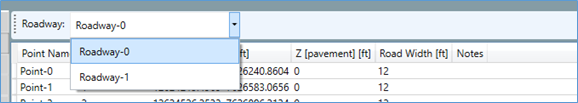
To adjust the z-coordinates of points of objects, we go to the Objects Detail pane and select the tab on the bottom that relates to the object we want to edit, for example if we want to edit the z-coordinate of one of the roadway objects we would select the Roadways tab. For all objects except the receiver objects, we would then select the Points tab on the left-hand side. (The other tabs present on the left side will depend on what type of object you have selected in the lower tabs.) For the receiver objects, the z-coordinates are accessible in the Receivers tab. If the object has not been selected do so now by selecting it from the dropdown menu. (See figure below.)
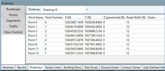
Once the specific object has been selected, the grid will be populated with data related to the points for this object. An example is shown for a roadway in the figure below. For the time being, we will assume that the ground around the project all has the same elevation, so we can leave the z-coordinates for all objects at the same relative value, e.g. 0 ft.
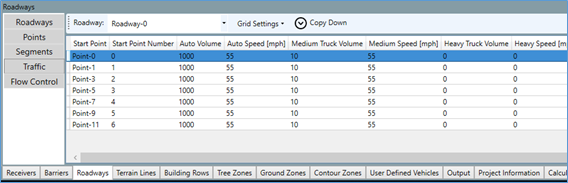
To add traffic to each roadway, go to the Roadways tab at the bottom. On the left side of the pane there will now be five tabs pertinent to roadways. To add traffic to the roadway, select the Traffic tab on the left. You will then see a table that has 0 for all traffic volumes and speeds. Each cell can be edited directly. It is often easiest to enter the traffic volumes and speeds for the first row of data and the use the Copy Down function at the top of the Object Details pane to copy these data. The figure below shows some sample traffic data. Add traffic to both roadways.
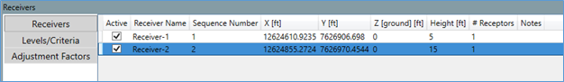
Next, examine the receivers using the Objects Detail pane by selecting the Receivers tab at the bottom of the pane. Let's assume that the second receiver is on the second floor. We will want to increase the height of the receiver. This can be done in the Receivers tab on the left-hand side, i.e. select the Receivers tab at the bottom of the Objects Detail pane and then select the Receivers tab at the left of the Objects Detail pane. Note that there are two ways the height of the receiver can be changed. The z-coordinate can be changed (Z[ground]) and the height of the receiver above the ground (Height) can be changed. If you change Z[ground] then the geometry of the model will be changed, effectively adding a slope in the terrain between the receiver and the next object in the propagation path. This is not what we want to do here, rather we want to tell TNM that we are interested in the level a certain height above the ground, thus we need to edit the Height. The figure below shows the two receivers, each having a different height above the ground.
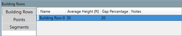
Next, we want to set the height of the Building Row. Select the Building Rows tab at the bottom of the Object Details pane and then select the Building Rows tab on the left. Make sure that the Building Row is selected in the dropdown menu. Just like the receivers, the z-coordinate (found in the Points tab) affects the terrain between this object and the nearest objects along the propagation path. We want to affect the actual height, so we adjust the Average Height in the Building Rows tab on the left. Let's set the Average Height to 30 feet. Note, we can also increase the spacing between buildings in the Building Row by adjusting the Gap Percentage. We will leave the gap percentage at 20%. (Gaps less than 20% should use Barriers instead of Building Rows.) The settings for this object should look like the figure below.
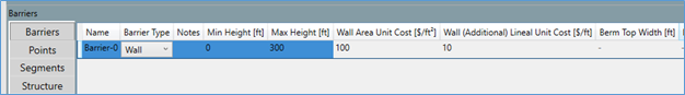
Now let's finalize the barrier. Select the Barriers tab at the bottom of the Object Details pane. The Barriers tab on the left allows you to select whether the barrier is a Wall or a Berm. If it is a berm, then more of the parameters in this grid are applicable. (If you switch back and forth between berm and wall, TNM will remember the settings that you entered while the object was set as a berm even though they are not displayed when set as a wall.) For this walkthrough, we will work with a Wall type barrier. In this case, we can set the Wall Area Unit Cost and Wall (Additional) Lineal Unit Cost. Set these to 100 $/ft2 and 10 $/ft respectively. The grid should look similar to the figure below.
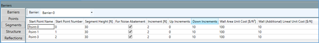
Next, we want to tell TNM to start compute the effect of the barrier for more than one height. We do this by going to the Segments tab on the left and setting the input heights in Segment Height to a desired height. Let's start the computations with a large value for the Segment Height, e.g. 30 ft. We will then tell TNM to compute the effect of the barrier for different combinations of heights for each segment. To do this set the Increment to 2 ft, leave the number of Up Increments at 0 and set the number of Down Increments to 10. For this example, when TNM computes levels for the receivers, it will start with all segments of the barrier at 30 feet and store these values. It will then reduce one segment by 2 feet and re-compute the levels and store these values, it will continue perturbing the segments until all combinations have been evaluated, e.g. 30, 30, 30 ft; 28, 30, 30 ft; 26, 30, 30 ft; ... 10, 30, 30 ft; 30, 28, 30 ft; ... 30, 10, 30 ft; 28, 28, 30 ft, ... 10, 10, 10 ft. Adding perturbations greatly increases the number of computations. To keep runtimes reasonable, choose perturbations carefully. The Segments grid for or example is shown in the figure below.
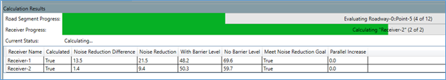
At this point our project is ready to be run. Go to the Calculate tab in the TNM Toolbar and select All Receivers. As the calculations are done, TNM will switch the bottom panel to show the Calculation Results, as shown in the next figure. Here the top bar shows the progress for the current receiver and the lower bar shows the progress for the receiver list.
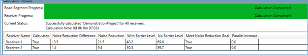
The next figure shows the completed calculations. The table below the progress bar will be updated to show the results for each receiver. Note, it will take a few seconds for this to update after the calculations are completed.
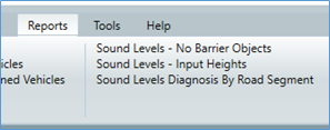
There are a number of reports that the user can view once TNM has finished its calculations. These reports can be opened by selecting the desired report from the Reports menu (shown below).
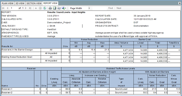
For example, selecting the report, Sound Levels – input Heights, will generate a report in the View Pane in the Report View as shown in the next figure. Note that these reports can be printed directly from the Report View or they can be exported to many common formats. To print or export the report use the options in the ribbon just below the Report View tab.
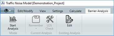
The Barrier Analysis tool allows the user to precompute receiver levels for all combinations of barrier heights for each segment, as was discussed in the Objects Detail Pane section. Once TNM has computed all of the possible combinations, the user can then start a new Barrier Analysis. To do so, select the Barrier Analysis tab and click on the Start Analysis icon.
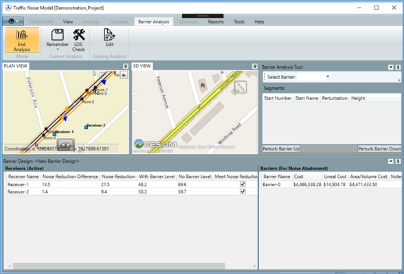
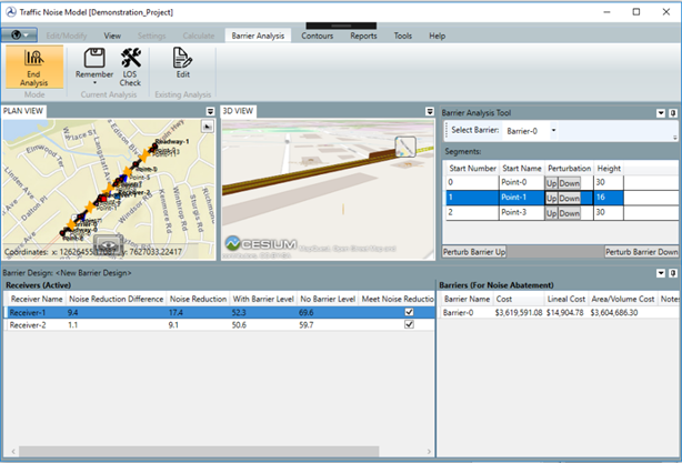
Pressing the Start Analysis icon will change the layout of TNM to the form shown in the next figure. This layout is designed to be able to perturb selected barriers through their precomputed perturbations while at the same time seeing how these changes affect the receiver levels and the geometry. The Plan View is still enabled and this can facilitate selecting a particular receiver. The 3D View can be used to see what the current design would look like. You can manipulate the orientation of the 3D View by holding down the scroll wheel while in the 3D View and moving the mouse around to get a good perspective of the barrier that you are interested in. The lower panels show the results for each receiver for the barrier design and cost for the design. The Barrier Analysis Tool panel, in the upper right, is where most of the user interaction will take place.
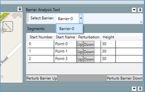
The user can select a barrier to perturb in the Barrier Analysis Tool as shown in the next figure. When the barrier is selected the segments that can be perturbed will be listed. There will be buttons for perturbing each segment up or down and a column that indicates the height for the current design. Note that the entire barrier can be perturbed up or down inside the tool by utilizing the buttons on the lower left and lower right. When a barrier segment has reached the end of its perturbed heights (either the upper limit or lower limit) it will remain at this height for any further perturbations in this direction.
The next figure shows the Barrier Design Tool as initialized with all barrier segments at input heights. Note, the levels in the lower panel for each receiver and the geometry of the design in the 3D View.
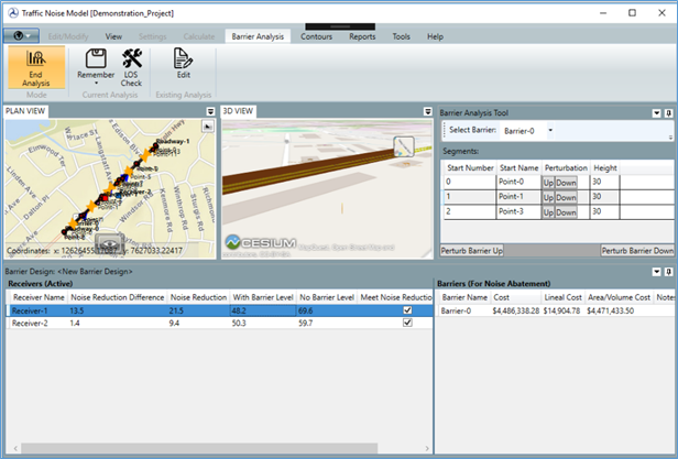
The next figure shows a barrier design for this barrier where the middle segment has been perturbed down from its input height of 30 ft. to the design height of 16 ft. Notice the difference in receiver levels and in the geometry in the 3D View.
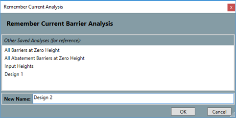
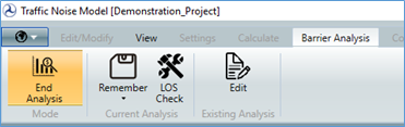
Once a barrier design of interest has been designed, it should be saved. This is done by clicking on the Remember icon in the Barrier Analysis tab.

This will open a dialog where a name can be entered for the new design. Press OK after entering the desired name.
Pressing End Analysis returns TNM to the normal layout.
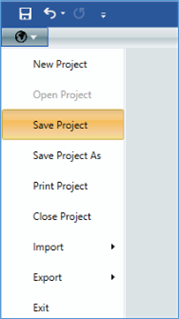
Finally, remember to save the entire project by clicking on the World tab and selecting Save Project.
This concludes the walkthrough. You should now be able to
Further details and functionality can be explored by using the User's Guide in the Help Menu.

