

| << Previous | Contents | Next >> |
Relationships Between Asset Management and Travel Demand:
Findings and Recommendations from Four State DOT Site Visits
3.1 Introduction
Chapter 2 described the movement to adopt TAM within state DOTs and recent trends in U.S. highway travel demand growth. Given that background, this chapter describes the specific questions addressed by this study and the approach taken in evaluating how a sample of four state DOTs are applying TAM principles to the issue of continued growth in travel demand. This chapter also describes the process used to identify the four sample states selected for this project and provides a brief analysis of the varied highway network and travel demand characteristics of each of these states.
3.2 Study Objectives
This study seeks to determine whether and how state DOTs are using TAM and related techniques to address the issue of existing and anticipated future travel demand. Correspondingly, this study attempts to identify and document all cases in which state DOTs have incorporated travel demand measures within TAM and related analyses and decision-making processes. This includes those instances in which current and projected travel demand measures are used as inputs to TAM processes as well as those instances where a mitigated travel demand-related problem is the intended output of a TAM process (see Exhibit 3-1).
| Travel Demand Inputs (current and forecast) | State DOT TAM Processes (Existing and Potential) | Travel Demand Outcomes (current and forecast) | ||||
|---|---|---|---|---|---|---|
| User of Travel Demand Measures as Inputs | Impact Travel Demand Related Outcome | |||||
Auto and Truck VMTs AADTs Level of Service (LOS) Travel Delay Cost |
⇒ | Incident Management Prioritization of Preservation Activities (e.g., by location based on current VMTs) Current and Projected Infrastructure Deterioration (e.g., Roadway Wear) Major Project Cost Effectiveness and Alternatives Analysis |
Investment Trade-Offs (Capacity, Preservation, Safety) Performance Measures and Standards Long-Term Planning and Budgeting |
⇒ | Reduced Congestion Reduced Travel Time Increased Efficiency Improved Safety |
|
At a minimum, the study set out to determine how state DOTs are addressing the following issues:
Current and projected travel demand measures as inputs to the TAM process
- Infrastructure deterioration (e.g., roadway wear): Increasing traffic volumes and vehicle weights result in increasing rates of roadway deterioration. How do state DOTs take current and projected travel demand measures into account when evaluating the current maintenance and rehabilitation needs of existing roadway infrastructure? Are state DOTs using current and/or projected travel demand measures to help project the timing and magnitude of future rehabilitation and replacement needs?
- Investment prioritization: The benefits of reinvesting in existing infrastructure tend to be highest for segments with relatively greater customer utilization. How are state DOTs using TAM and related techniques to prioritize roadway re-investment between and within regions based on current and projected future utilization?
- Project benefit-cost and alternatives analysis: The cost-effectiveness (or return on investment) of major new investments and the relative benefits of project alternatives are heavily influenced by travel-time savings. How are state DOTs incorporating travel-time savings into their selection processes for major projects?
Using the TAM process to address issues related to travel demand
- Capacity improvements: As noted above, the rate of growth in travel demand remains well above the rate of growth in roadway capacity, leading to increasing congestion and travel times. Have state DOTs adopted TAM-related practices to help identify capacity improvement strategies or for prioritizing potential expansion investments?
- Safety improvements: Increasing roadway utilization also brings increasing opportunities for crashes, injuries, and fatalities. How are the safety implications of current and future travel demand for both light-and heavy-duty vehicle traffic factored into system management decisions?
- Trade-offs between preservation and capacity needs: All state DOTs face the problem of balancing re-investment in existing roadway capacity with the need for additional capacity to address growing demand - all within limited financial resources. How have TAM and related processes been used to allocate funds between these and other competing needs, and how do travel demand measures inform this allocation?
- Objectives and performance measures: TAM emphasizes the need to establish long-term system objectives and to develop processes and measures to evaluate success in attaining those objectives. How do state DOTs propose to measure and report performance relative to travel demand? Have they identified or established desired performance standards with respect to roadway volumes, congestion, and other travel demand-related measures? If not, why?
- Long-term planning and budgeting: TAM emphasizes the need to take a long-term, strategic view in establishing attainable organizational objectives within realistic resource constraints. Given these objectives, how do state DOTs incorporate travel demand forecasts into their long-term investment plans? How are those plans constrained by existing resources? How are long-term travel demand and budgeting concerns incorporated into agencies' strategic plans? How long is the long-term?
3.3 Study Approach and Sample States
The study collected data on the asset management, travel demand forecasting, and related practices of four state DOTs: California (Caltrans), Michigan (MDOT), North Carolina (NCDOT), and Utah (UDOT). The study team conducted two to three full days of interviews with key staff at each agency, including asset managers, travel demand modelers, short- and long-range planning staff, short- and long-range programming and budgeting staff, roadway maintenance staff, operations personnel, and IT and database maintenance staff. Interviews were intended to fully document the following:
- The extent and maturity of each state's asset management program
- Structure and role within broader DOT organization
- Program goals and objectives
- History and development
- Capabilities
- Future plans
- Dedicated resources
- How DOTs use TAM to address travel demand issues
- Collection of current and projected travel demand measures
- Uses of travel demand measures in support of asset management
- Intermodal, interstate, and international traffic flow considerations
- Current operations and maintenance
- How DOTs address their long-term investment needs
- Long-term transportation planning
- Long-term budgeting
- Strategic transportation planning (how does asset management inform or shape each state's infrastructure and financial plans?)
The sample states were selected to provide a broad representation of highway network features, travel-demand characteristics, system size, population growth, urban concentration, industry, climate, and topology. States were also selected to include some of the more advanced in the adoption of TAM practices.
The selected states of California, Michigan, North Carolina, and Utah provide a broad cross-section of state highway and travel-demand characteristics nationwide. For example, this group of states encompasses a wide range of state-maintained highway networks (NCDOT is responsible for close to 170,000 lane-miles versus just 15,000 for UDOT), varying shares of urban versus rural roadways (25 percent of Caltrans-maintained highways are urban versus just 12 percent for NCDOT), a range of population and VMT growth rates (urban annual VMT growth is just over 2 percent in California and Michigan but exceeds 3 percent in Utah and North Carolina), and wide variations in congestion (urban AADT per lane mile exceeds 17,000 in California but is only 4,000 in North Carolina).
3.3.1 Asset Management Plan Development
In addition to including states considered among the more advanced in adopting TAM practices, the selected states have also emphasized varying practices. For example, Michigan is the most advanced in data collection and dissemination, Utah has emphasized the development of decision-support tools, and California is focused on the development of state-wide performance monitoring. North Carolina has placed less emphasis on specific goals (and hence, has less capabilities than some other states in specific areas) but more effort on embracing a more comprehensive asset management approach.
Although each of these states has made strong progress in adopting specific asset management practices, none has fully implemented a program that encompasses all TAM functions as outlined earlier in Exhibit 2-1 (i.e., including well-defined program goals and polices; comprehensive asset inventory; decision-support tools; comprehensive long-range strategic planning and budgeting; and full program optimization across all asset types, regions, and investment types). Rather, each of these state DOTs is working towards development of comprehensive TAM programs and the further refinement of its existing processes. Moreover, the development of their existing programs clearly represents many years of sustained investment, and the successful implementation of new improvements will similarly require considerable effort. The evidence from this study suggests that these investments are clearly paying off in the form of better data, credible analyses, and more informed decision making.
3.4 Characteristics of the Participant States
Exhibit 3-2 presents the characteristics of each of the states participating in the study: California, Michigan, North Carolina, and Utah. Brief descriptions follow.
| State | California | Michigan | North Carolina | Utah |
|---|---|---|---|---|
| General Characteristics | ||||
| Population (Millions) | 34.7 | 10.1 | 8.0 | 2.2 |
| Projected Annual Population Growth | 1.3% | 0.5% | 1.5% | 1.8% |
| Area (Square Miles) | 163,707 | 96,810 | 53,821 | 84,904 |
| Population Density (population per square mile) | 212 | 104 | 149 | 26 |
| Gross State Product ($Billions) | $1,359 | $321 | $276 | $70 |
| Roadway Miles: Total | 169,793 | 122,381 | 102,666 | 42,712 |
| Mean Travel Time to Work (Minutes) | 27.7 | 24.1 | 24.0 | 21.3 |
| State Controlled Roadways: Infrastructure | ||||
| Roadway Miles | 15,209 | 9,720 | 78,871 | 5,858 |
| State Controlled Share of Total Roadway Miles | 9.0% | 7.9% | 76.8% | 13.7% |
| Lane Miles | 50,522 | 27,578 | 168,029 | 15,260 |
| Annual Growth in Lane Miles | 0.2% | 0.3% | 0.3% | 0.3% |
| Lane Miles Per Roadway Mile | 3.32 | 2.84 | 2.13 | 2.60 |
| Urban Share of Total Lane Miles | 42% | 39% | 14% | 25% |
| Bridges | 24,007 | 10,879 | 17,509 | 2,815 |
| State Controlled Roadways: Expenditures | ||||
| Capital Outlays ($M) | $4,130 | $1,095 | $1,834 | $451 |
| Maintenance and Services ($M) | $708 | $245 | $570 | $107 |
| Expenditures per Lane Mile ($000) | $95.8 | $48.6 | $14.3 | $36.6 |
| State Controlled Roadways: Travel Demand | ||||
| Daily VMT (in thousands) | 502,858 | 159,951 | 227,536 | 47,575 |
| Annual Growth in Daily VMT (1994 to 2004) | 2.5% | 2.8% | 2.9% | 3.0% |
| AADT per Lane | 9,953 | 5,800 | 1,354 | 3,118 |
| Annual Growth in AADT per Lane (1994 to 2004) | 2.2% | 2.2% | 2.6% | 2.7% |
3.4.1 California
California's geography is perhaps the most diverse of all 50 states. In addition to a mountainous perimeter and Central Valley dominated by a fertile plain, California also features more than 800 miles of ocean coastline and several of the nation's largest urban areas. The state also experiences widely divergent climate including from desert in the south, rain forest along the northern coasts, and high alpine terrain on its eastern border.
California is also an economic powerhouse. With a gross state product of more than $1.4 trillion annually, California produces more than 13 percent of the nation's total goods and services and is frequently touted as the world's sixth largest economy. The state is also home to several large ports, including those in Los Angeles/Long Beach and Oakland, which directly support international trade flows between Asia and the 48 contiguous states. The state is also a major provider of fresh produce to the rest of the nation. With more than 34 million people, California is the nation's most populous state. Population is projected to grow at an average annual rate of 1.3 percent over the next 20 years.
With over 169,000 miles of roadway and more than 24,000 bridges, California is home to the nation's second largest roadway network (after Texas). Maintenance, preservation, and expansion of this large network pose special problems and conflicting demands on state resources ranging from high traffic demand in multiple urban areas to heavy snow removal requirements in mountainous regions. This network is also characterized by one of the nation's largest concentrations of lane miles in urban areas and a very high proportion of multi-lane highways relative to other states.
The problem of traffic congestion on California's urban highways is well documented and projected to worsen in the future given ongoing increases in population and economic development. Mitigation of this problem is a special challenge given the maturity of the state's existing urban roadway networks. One consequence of the state's urban congestion is ongoing urban expansion and the development of previously rural areas.
3.4.2 Michigan
The Great Lakes divide Michigan into two large peninsulas, both located north of the nation's major east-west transportation corridors. Michigan's economic success depends on a sound multimodal transportation system to provide access for people and goods both to the rest of the nation and across the border into Canada.
Michigan has over 120,000 miles of statewide highways and more than 11,000 bridges. A significant challenge facing MDOT is Michigan's unusual climate. The lakes modify the severe northern winter weather, leading to heavy lake effect snows and frequent freeze-thaw cycles. The results are rapid infrastructure deterioration, high maintenance costs, and a small window for road construction activities. Under these conditions, investments that extend the life of existing facilities and improve the performance of the transportation system are essential for Michigan's citizens and economic sector to prosper. MDOT's asset management process focuses on these objectives.
Michigan is currently home to more than 10 million people, and the state's population is expected to grow at an average annual rate of 0.5 percent through 2025. While Michigan has the lowest rate of population growth among the four sample states, it continues to experience strong VMT growth, particularly in the state's urban areas. With modest expansion in the existing roadway network, this ongoing growth in travel demand is also yielding related increases in congestion, travel delays, and lost productivity, most notably in the urbanized areas surrounding Detroit.
3.4.3 North Carolina
North Carolina's geography is representative of the nation's Mid-Atlantic states, including a mountainous west, a rolling piedmont mid-section, and a flat coastal plain in the east. While the state's climate is considered mild relative to the many extremes within the U.S., the state is subject to long, hot summers, which accelerate the process of asphalt drying and deterioration.
North Carolina's economy has undergone extensive growth in recent years, moving beyond the state's traditional industries, such as tourism and agriculture, to embrace higher-paying, service-sector employment relating to banking and the region's growing research centers. North Carolina's gross state product is roughly $270 billion annually. The state is currently home to 8 million people, and its population is expected to grow at a robust 1.5 percent average annual rate through 2025.
North Carolina has over 100,000 miles of statewide highways and more than 17,000 bridges. In stark contrast to the other states included in this study, the state's department of transportation, NCDOT, is responsible for the maintenance and operation of more than 75 percent of the state's roadway network and bridges (versus an average of roughly 10 percent for the other study states). Responsibility for such a large share of the state's aging highway network places unusually high demands on NCDOT's highway resources. Also in contrast to the other study states, North Carolina's highway network continues to expand by more than 400 miles per year due to: (1) a legislative requirement to build out the state's intrastate highway network, (2) continued paving of rural dirt roads, and (3) NCDOT's responsibility to maintain roads constructed for housing developments located outside of municipal boundaries. These growing challenges are central to the department's strong interest in the initial development and ongoing improvement of its asset management program.
While the state's traffic congestion problems may be considered minor relative to those of California or even Michigan, these issues will become more significant if not addressed in the near term. As already noted, North Carolina continues to experience strong population growth. Moreover, the state's rate of growth in VMTs and AADT per lane is also larger than that experienced by either California or Michigan (although smaller than Utah's).
3.4.4 Utah
Utah's geography is unique within the sample of states in this study in that it does not border any major bodies of water or reside on an international border or international waterway. Rather, Utah is "land-locked" and centrally located. Consequently, much of the traffic on interstate highways flows through the state (rather than originating and/or terminating within the state as with California, Michigan, and, to a lesser extent, North Carolina). The state also features a broad range of terrains including high mountain ranges, salt flats, and a rugged desert. These extremes in elevation and terrain also bring wide variation in temperature and snowfall.
Of the four states included in this study, Utah has the smallest economy (an annual gross state product of $70 billion), the smallest population (2.2 million), and by far the lowest population density (26 per square mile versus 212 for California, 104 for Michigan, and 149 for North Carolina). The vast majority of the state's population, economic activity, and growth is located along the western boundary of the Wasatch Front stretching between Ogden, Salt Lake City, and Provo. Within this corridor, population densities and the resulting congestion are comparable to the nation's other urbanized areas. Moreover, with projected average annual population growth of 1.8 percent (the highest of the sample states) and the confining influences of mountains on the east and Salt Lake and Provo Lake to the west, population densities and travel demand within this corridor are expected to continue growing. Over the period from 1994 through 2004, Utah's state-maintained highways exhibited the fastest overall rates of growth in both VMT and AADT per lane among the four states included in this study.
With only 43,000 miles of statewide highways, Utah has the smallest public roads network of the four study states. UDOT is responsible for operation and maintenance of just under 6,000 miles of road and fewer than 3,000 bridges. With the state's population and economic activity centered on the Salt Lake City region, very low population densities in the rest of the state, and wide variations in climate, UDOT faces unique challenges when attempting to prioritize capital investments and maintenance resources within and across regions. A key motivation in adopting asset management practices was to determine how best to allocate transportation resources both optimally and equitably.
3.5 Comparative Analysis of State DOT-Operated Highways
Exhibit 3-2 provides a range of statistics comparing the economic, geographic, demographic, highway network, and travel demand characteristics of the four sample states. This sub-section considers several of these measures in greater detail, with emphasis on the relative levels and rates of growth in network size and travel demand on state-controlled highways (i.e., the network that state DOTs control).
Exhibit 3-3 compares the total number of lane-miles within each of the four sample states as well as the share of those lane-miles that are owned and maintained by the state DOT. Although California has the largest highway network, with close to 380,000 lane miles statewide, North Carolina has by far the largest number of state-maintained highways (both as a proportion of statewide miles and in total lane-miles maintained). The high share of state-maintained lane-miles within North Carolina places high demands on the state's highway resources (with more highway miles to maintain per dollar of funding) and has also required a closer working relationship between the state and local governments than is the case in other states (i.e., to manage and prioritize preservation and expansion projects).
Exhibit 3-3: Total lane-miles statewide in sample states (Description)
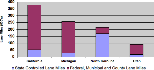
Exhibit 3-4 presents the number of state-controlled lane-miles operated by each of the four sample states over the period 1994 to 2004. As with the national trends depicted in Chapter 2, the number of state-controlled lane-miles within each of these four states has grown very slowly over the past decade, averaging roughly 0.2 percent to 0.3 percent annually for each of the four states. However, given its large existing highway network, small percentage increases in North Carolina's network translate into significant investment in new lane-miles relative to the other study states. This situation is apparent in Exhibit 3-5, which shows that North Carolina's roadway network increased by close to 450 miles each year over the last decade. This rate of increase was more than 3 times that of California, more than 5 times that of Michigan, and more than 10 times that of Utah.
Exhibit 3-4: State-controlled lane-miles in sample states (Description)
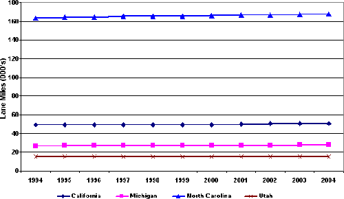
Exhibit 3-5: Average annual increase in state-controlled lane-miles (Description)
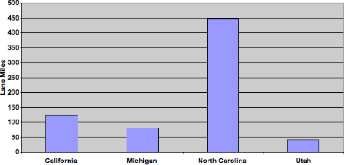
Exhibit 3-6 presents the proportion of state-controlled lane-miles within each of the four sample states that are located in urban areas. Of the four states, California maintains by far the highest number of urban highways as a share of total state-maintained highways. California, Michigan, and Utah have each experienced slow, long-term increases in the proportion of state-maintained urban highways (the recent jump in shares for Michigan and Utah reflect recent reporting changes due to the 2000 Census). By contrast, North Carolina's state-controlled highways are clearly dominated by rural roadways and the state's share of urban roadways remains flat, due most likely to state control of local roads in non-urban areas.
Exhibit 3-6: Percentage of state-controlled highways located in urban areas (Description)
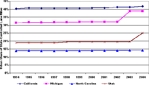
The characterization of each state's highways into urban and rural types is important to this study. Travel demand-related issues of traffic congestion, increasing travel times, and lost productivity are primarily urban issues; therefore, any state efforts to monitor and mitigate these issues will necessarily be focused on urban areas.
Exhibit 3-7 documents the levels and rates of increase in daily VMTs on state-controlled highways within the four sample states over the past decade. California's state-maintained highways carry significantly more traffic as compared to the three other states. Moreover, while each of the four states experienced an annual growth rate in daily VMTs of between 2.5 percent and 3.0 percent over the period 1994 to 2004, California's state-maintained roads have clearly experienced the largest annual increase in the number of VMTs. Specifically, over the last decade, the average annual change in daily VMTs for California was 10.9 million. Comparative figures elsewhere include annual increases of 5.6 million for North Carolina, 3.5 million for Michigan, and 1.2 million for Utah. The large number of VMTs and significant growth in VMTs for North Carolina reflect the large number of state-controlled lane-miles in that state.
Exhibit 3-7: Daily VMT on state-controlled highways (Description)
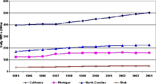
Exhibit 3-8 documents the levels and rates of increase in AADT per lane on state-controlled highways within the four sample states over the past decade. In effect, Exhibit 3-8 normalizes the daily VMT measures presented in Exhibit 3-7 to reflect the wide differences in total state-maintained lane-miles within each state and the widely varying implications for roadway utilization, traffic congestion, roadway deterioration, and safety.
Exhibit 3-8: AADT per lane on state-controlled highways (Description)
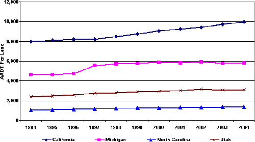
Exhibit 3-8 demonstrates that lane-mile utilization is significantly higher in California than the other three states. However, regardless of differences in existing AADT per lane values across these four states, the annual rate of increase in AADT per lane is well over 2 percent for each state (2.2 percent for California and Michigan, 2.6 percent for North Carolina, and 2.7 percent for Utah), reflecting the increasing divergence between growth in travel demand and lack of growth in physical capacity. Over the period 1994 to 2004, the average annual increase in AADT per lane was highest for California and Michigan (at 196 and 115 vehicles per day, respectively) and lowest for Utah and North Carolina (at 73 and 31 vehicles per day, respectively).
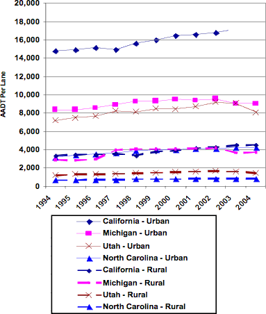
Exhibit 3-9 segments the AADT per lane data from Exhibit 3-8 into their urban and rural components. Aside from highlighting the significantly higher level of highway utilization in urban versus rural areas, this exhibit also demonstrates the relatively low level of utilization for North Carolina's highway network (e.g., where urban AADT per lane is comparable to rural roadway utilization in California and Michigan).
Exhibit 3-9 summarizes the differences between the historic rates of growth in lane-miles, VMTs, and AADT per lane for all four states. This exhibit also further segments these rates into their urban and rural components. Once again, this presentation emphasizes the low rate of growth in lane-miles relative to the more rapid increase in travel demand (as measured by VMT), yielding an overall increase in highway utilization (as measured by AADT per lane). Interestingly, while the rate of increase in VMTs has been higher in urban areas, rural areas have experienced higher rates of growth in AADT (with the exception of North Carolina). This trend may reflect ongoing suburban expansion or "sprawl" beyond traditional urban boundaries.
Exhibit 3-9: AADT per lane on urban versus rural state-controlled highways (Description)
Several of the preceding exhibits have emphasized variations in the current levels and rates and growth in roadway utilization across the four sample states, particularly in urban areas. As may be expected, these variations translate into varying levels of congestion and travel delay costs. Exhibit 3-11 provides estimates of the total annual hours of travel delay for select urban areas located within each of the four sample states (based on analysis from the Texas Transportation Institute's 2005 Urban Mobility Report). It is important to note that this analysis is not inclusive of all urban areas within each state. Moreover, the analysis measures travel delay across all highways and not just those maintained by the state DOTs. Nevertheless, this travel delay analysis does accurately depict the congestion issues faced by each state DOT within its state's urban areas. For example, Exhibit 3-11 makes it clear that California must address congestion delay issues of greater magnitude (particularly in the region surrounding Los Angeles) and in more urban areas than any of the other four study states.
| State | California | Michigan | North Carolina | Utah |
|---|---|---|---|---|
| Lane Miles | ||||
| Urban | 0.6% | 0.6% | 0.4% | 0.6% |
| Rural | 0.0% | 0.2% | 0.2% | 0.1% |
| All | 0.2% | 0.3% | 0.3% | 0.3% |
| VMTs | ||||
| Urban | 15,209 | 9,720 | 78,871 | 5,858 |
| Rural | 9.0% | 7.9% | 76.8% | 13.7% |
| All | 50,522 | 27,578 | 168,029 | 15,260 |
| AADT per Lane | ||||
| Urban | $4,130 | $1,095 | $1,834 | $451 |
| Rural | $708 | $245 | $570 | $107 |
| All | $95.8 | $48.6 | $14.3 | $36.6 |
While Exhibit 3-11 captures the total travel delay within each urban area (reflecting both the average delay time for each traveler and the number of travelers), Exhibit 3-12 depicts the estimated travel delay on a per-traveler basis. This exhibit also highlights the greater magnitude of California 's traffic congestion issues statewide, and effectively demonstrates the high cost of traffic congestion to individual travelers within each of the four sample states.
Although congestion is primarily a function of the number of vehicles on the road, infrastructure deterioration is primarily a function of the composition of those vehicles, with truck traffic contributing most to the rate of pavement wear. Exhibit 3-13 presents truck traffic as a share of total VMTs for urban and rural highways in each of the four sample states as well as for the nation as a whole. This exhibit demonstrates that while urban truck traffic represents a relatively consistent share of total VMTs across each state, there is significantly greater variation in trucks' share of rural VMTs. In particular, trucks account for a very high proportion of rural VMTs in Utah, reflecting both the low rural population densities and the large volume of truck traffic flowing through the state.
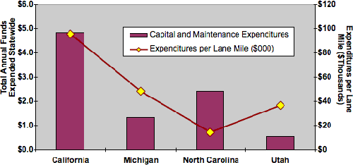
This comparative analysis has focused on the characteristics of the roadway networks, travel demand, and congestion of the four sample states. By contrast, Exhibit 3-14 compares the levels of capital, maintenance, and operations expenditures on state-maintained roadways within each sample state. Based on 2004 data, California expends more total funds on roadway operations, maintenance, and capital outlays, while Utah spends the least. When expressed on a per-lane-mile basis, California spends roughly $95.8 thousand per lane-mile on these activities, while North Carolina, with its very large state-maintained highway network, spends a more modest $14.3 thousand per lane mile. Michigan and Utah fall between these two points, spending $48.6 thousand and $36.6 thousand per lane-mile, respectively.
Exhibit 3-11: Total annual travel delay in sample state urban areas (Description)
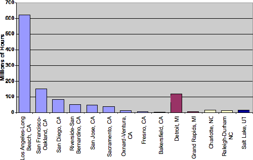
Exhibit 3-12: Annual delay per traveler in sample state urban areas (Description)
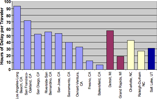
Exhibit 3-13: Truck traffic as a share of statewide VMTs (Description)
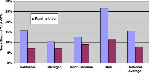
Exhibit 3-14: Capital and maintenance expenditures from federal, state and local sources (2004) (Description)
| << Previous | Contents | Next >> |