U.S. Department of Transportation
Federal Highway Administration
1200 New Jersey Avenue, SE
Washington, DC 20590
202-366-4000
Federal Highway Administration Research and Technology
Coordinating, Developing, and Delivering Highway Transportation Innovations
| REPORT |
| This report is an archived publication and may contain dated technical, contact, and link information |
|
| Publication Number: FHWA-HRT-09-028 Date: May 2009 |
Publication Number: FHWA-HRT-09-028 Date: May 2009 |
Through both physical experiments and CFD simulation, the forces exerted on the three bridge deck types were analyzed in detail. Before analyzing the performance of the CFD models in estimating the force values, it was important to verify qualitatively that the flow fields generated in the CFD models matched those produced in the PIV experiments. The first section of this chapter describes these comparisons.
The following sections display the results of the experimentation and the CFD simulation on design charts showing the relationship between the inundation ratio (h*) and the unitless coefficients for drag, lift, or moments. The experimental results represent averages of three to five trials performed for each Fr at each inundation ratio. To further expand results, the data were used to calculate parameters for fitting equations which roughly bound the high- and low-force coefficients values. These equations are shown in the drag, lift, and moment plots as blue lines and are also referred to as envelope curves since they generally form and envelope around the experimental results. The form and coefficient values of these equations are laid out in the final section of this chapter.
Figure 22 through figure 27 show comparisons of the simulated velocity contours around the bridge deck to the PIV measurements from the experiments for each bridge type.
The PIV measurements were conducted with smaller scale bridge decks, which were smaller by the factor of 1.5 from the bridge deck used in the evaluations of hydrodynamic forces. The flow conditions compared were for V = 250 mm/s with hu = 50 mm, 101 mm, and 116 mm and the depth of the flow, hu, as 170 mm. Each PIV image was matched with a velocity map from the CFD model simulated with a similar value of h*. The velocity profiles show the velocity of the water in the direction of flow across the bridge cross section. Red indicates high velocity, while orange, yellow, green, and blue represent progressively slower velocities. Darker blue areas indicate where the flow was not moving or moving in reverse during the experiment, possibly indicating the presence of a stable vortex. The flow field vectors were drawn in both maps, but the PIV vectors were not connected into streamlines as the CFD results were.
In general, the velocity profiles show strong agreement between the flow fields. The three bridge types show noticeable differences. The three-girder bridge easily produced the most substantial vortex zones, with a particularly strong one just downstream of the third-girder bridge. Additionally, the three-girder bridge had a larger zone of no-flow than the six-girder bridge just downstream of the first girder. The six-girder bridge appeared to create a larger disturbance on the top of the bridge, however. Both of these phenomena were most easily seen in the PIV profiles.
The streamlined bridge deck had a much smaller impact on the velocities than the other two deck shapes. As flow encountered the first lobe, there was evidence of contraction-induced acceleration as the velocity above and below increased slightly. The CFD and PIV results for the streamlined bridge differed somewhat in the location of the primary flow obstructions. The CFD results place two small but noticeable vortices (shown in figure 26) on the downstream edge of both short triangular guardrails. There was virtually no reduction in flow velocity beneath the bridge. The PIV results, however, display a significant zone of very slow flow in the cavity on the underside of the streamlined deck (shown in figure 27).
Overall, the velocities in the flow field seemed quite comparable between the CFD models and PIV experiments. Even minute differences in the flow fields or non-visible flow parameters, however, could lead to significant differences in the simulated force values. The next sections highlight the deck force results.
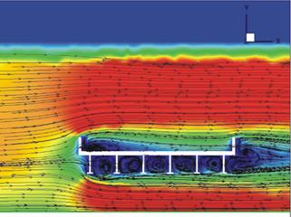
Figure 22. Image. Velocity profile from the Fluent® κ-ε CFD model for the six-girder bridge.
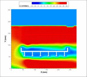
Figure 23. Image. PIV velocity profile for the six-girder bridge.
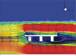
Figure 24. Image. Velocity profile from the Fluent® κ-ε CFD model for the three-girder bridge.
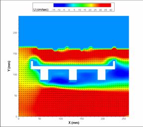
Figure 25. Image. PIV velocity profile for the three-girder bridge.
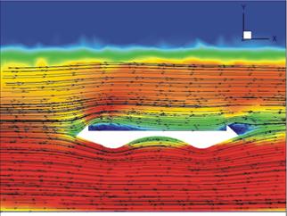
Figure 26. Image. Velocity profile from the Fluent® κ-ε CFD model for the streamlined bridge.
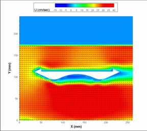
Figure 27. Image. PIV velocity profile for the streamlined bridge.
The six-girder bridge deck represented the dimensions of a typical highway bridge deck. The 1:40 scale of the model allowed the range of Fr used in the experimentation to correspond well with realistic Fr for actual flood flows interacting with bridges.
Figure 28 depicts the relationship of the inundation ratio with the drag coefficient, CD, for the six-girder bridge. The experimental data are shown in four series of points. The fitting equations are shown as lines, and the calibrated results of the STAR-CD® simulation and two Fluent® models are presented as points.
Figure 28. Graph. Drag coefficient versus inundation ratio for the six-girder bridge.
The drag coefficient plot shows that the drag coefficient was positive at all values of h* but that there was a major dip in the drag coefficient at h* around 0.5-0.8. This corresponds to a case when the bridge was slightly more than halfway inundated, perhaps as the water level was reaching the top of the girders and was beginning to transition to overtopping the deck. As the bridge became more inundated (h* > 1.5), the drag coefficient values leveled off to around 2.
The fitting equations enclose the experimental data generally well over the whole range of inundation ratios.
The CFD models did not show any dependence on Fr, so agreement with experimental data should not be overstated. The Fluent® κ-ε results showed very good agreement with the experimental data, replicating both the shape and magnitude, but slightly overestimating the maximum values. The Fluent® LES results generally provided low estimates of CD and did not increase quickly enough in the 1.0 to 2.0 range of h*. The STAR-CD® results showed good agreement at high inundation ratios but did not match the shape of the experimental data below h* = 2.
Figure 29 displays the lift coefficient plot for the six-girder bridge. Experimental data, fitting equations, and CFD simulation results are displayed in the same manner as in the drag coefficient plot. The experimental results revealed that the lift coefficient was negative for all the cases tested. A negative lift coefficient means that the flow was actually exerting a pull-down force on the bridge. While the effect was quite small when the water level was just barely reaching the bottom of the girders, the lift coefficient rapidly became more negative until h* roughly equaled 0.65. The lift coefficient slowly returned to 0 as the inundation ratio exceeded 3. As shown in figure 29, the fitting equations are generally representative of the experimental data but break down at higher inundation ratios and higher Fr.
Figure 29. Graph. Lift coefficient versus inundation ratio for the six-girder bridge.
The CFD model results did not closely follow the experimental results. The STAR-CD® results roughly captured the gradual increase in lift coefficient but fell below the bottom envelope curve. The two Fluent® models showed major departures from the experimental results' behavior and showed comparatively little influence from the inundation ratio. As shown in the figure, the Fluent® LES results are mostly flat when the experimental results show a considerable drop near h* = 1. Meanwhile, the Fluent® κ-ε start above the upper envelope curve but then roughly follow the experimental results at higher values of h*.
The moment coefficient plot is shown in figure 30. The experimental results demonstrate a similar shape no matter the Fr but are intriguing for their relative positions on the moment coefficient axis. There is little difference between the Fr = 0.16 and Fr = 0.22 cases, and both stay almost completely above 0. This corresponds to a moment rotating the bridge counterclockwise (rotating the upstream side of the bridge down and the downstream side up). The peak moment coefficient came during the study when the bridge was roughly halfway inundated, and the flow was pushing almost entirely on the first girder and thus below the center of gravity. At higher Fr, the effect was less pronounced. Additionally, in the 1.5-2 range for h*, the moment coefficient became negative and then stabilized for the Fr = 0.28 and Fr = 0.32 cases, which meant the bridge would turn over in the clockwise direction.
As shown in the figure, the CFD results demonstrate only fair agreement with the experimental results for the moment coefficient. Interestingly, the STAR-CD® and Fluent® κ-ε models show moderate agreement with each other. They also show reasonable agreement with some of the experimental results at high inundation ratios, but the moment coefficients are near 0 anyway. The Fluent® LES model has results consistently lower than the experimental Fr = 0.16 case. The model represents the reduction in the moment coefficient and stabilization but somewhat more aggressively than in the experimental results.
Figure 30. Graph. Moment coefficient versus inundation ratio for the six-girder bridge.
The three-girder bridge deck represented another common highway bridge design. The bridge-deck height was somewhat larger than the height for the six-girder, and the girders were rectangular and proportionally more massive. The increased deck height meant that the bridge could be tested for a narrower range of inundation ratios since the water depth remained at 0.25 m for all of the laboratory experiments.
Figure 31 shows the drag coefficient plot for the three-girder bridge. The experimental results display a shape similar to the results of the six-girder bridge, and the minimum point occurs at roughly the same inundation ratio. The two higher Fr cases (0.28 and 0.32) tend to group fairly closely, as do the two lower Fr cases (0.16 and 0.22). Additionally, the drag coefficient stabilizes at a higher value for Fr = 0.28 than for Fr = 0.32.
The CFD results for the three-girder bridge are also displayed on the plot in figure 31. Unlike the simulations for the six-girder bridge, the flow conditions in the CFD model are not calibrated based on the experimental results. Instead, the configuration of the six-girder model is used, and only the bridge deck model is changed. The STAR-CD® model results show only a slight response to Fr. The results, as plotted, seems to agree most closely with the higher Fr experimental results. The Fluent® results for the unsteady, 3-D κ-ε model display a general agreement with experimental results at lower h* values but somewhat overestimate the drag coefficient at higher values.
Figure 31. Graph. Drag coefficient versus inundation ratio for the three-girder bridge.
The lift coefficient plot in figure 32 shows a generally similar pattern to figure 29. The critical lift coefficient is slightly larger (more negative) for the three-girder deck. The three-girder deck shows a slightly more regular response to Fr as the experimental results do not cross each other nearly as much as in the six-girder experiments. The CFD results for both models replicate the lift forces fairly well, but the simulations do not capture the critical lift values.
The moment coefficient plot (figure 33) shows a similar shape to the moment plot for the six-girder bridge. The maximum positive moment occurs at an inundation ratio of approximately 0.8. The maximum moment coefficient value shown in the fitting is approximately 0.24, a reduction from the 0.30 coefficient for the six-girder bridge. This difference may be partially explained by the first girder being set back further from the leading edge of the bridge deck. At high inundation ratios, the direction of the moment reverses and attains a maximum value of negative 0.11 according to the fitting equations. Neither of the CFD models seems to capture the positive moment coefficients. The STAR-CD® model fits the experimental data reasonably well at high inundation ratios, but the Fluent® κ-ε model shows only weak agreement and a different shape.
Figure 32. Graph. Lift coefficient versus inundation ratio for the three-girder bridge.
Figure 33. Graph. Moment coefficient versus inundation ratio for three-girder bridge.
This section presents the results for the streamlined bridge deck. Only one CFD model, a Fluent® κ-ε model, was created for the streamlined bridge deck. As was the case with the three-girder deck, the flow configuration settings of the six-girder model were used for the streamlined deck because modeling results were not available for calibration.
Figure 34 shows the drag coefficient plot for the streamlined bridge deck. In contrast to the three- and six-girder bridge decks, the drag coefficients are significantly lower for the streamlined decks by a factor of roughly 50 percent. Additionally, the streamlined deck appears much less influenced by Fr, as all four sets of experimental results are tightly bunched. The experimental results have difficulty capturing data between 0.5 and 1 due to the model bridge deck's small profile. Nonetheless, the minimum drag coefficient value appears to occur at an inundation ratio of 1.2 versus roughly 0.8 for the other deck shapes.
The CFD results match the experimental results fairly well for the drag coefficient only. The CFD results for the lift and moment coefficient, however, do not match very well probably because the flow conditions were calibrated for the larger and differently shaped six-girder deck.
Figure 35 displays the lift coefficient plot. The data take a similar shape to the results for the other bridges. The critical value of roughly -1.2 represent a 20 to 25 percent reduction in pull-down force compared to the other two bridge shapes. The experimental results' variation by Fr is dramatic, as there appears to be a strong grouping among the Fr = 0.22, 0.28, and 0.32 scenarios but then a wide gap to the Fr = 0.16 scenario.
The streamlined bridge's moment coefficient plot (figure 36) exhibits different behavior than the other moment plots. Notably, the shape of the experimental results does not follow a smooth curve up to a peak and then a smooth decline but rather abruptly go to a peak. The peak location is not known precisely due to a lack of data at h* < 1, but the peak seems to occur at about h* = 1 or less, which is interesting because the critical points of the lift and drag plots occur at somewhat higher values of h*. The down slope of the experimental values also appears as two fairly linear segments (with a change to a flatter slope at roughly h* = 2.25), rather than the smooth curve exhibited by the six-girder data. Overall, though, it is evident that the peak moment coefficient on the upper envelope curve of roughly 0.2 is about a 33 percent reduction from the six-girder coefficient.
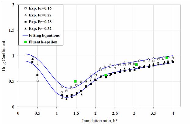
Figure 34. Graph. Drag coefficient versus inundation ratio for streamlined bridge deck.
Figure 35. Graph. Lift coefficient versus inundation ratio for the streamlined bridge.
Figure 36. Graph. Moment coefficient versus inundation ratio for the streamlined bridge.
This section provides the fitting equations for the curves shown on the plots and the necessary coefficient values to generate each fitting curve. The equation for each force or moment coefficient is given as a function of h*. The upper and lower fitting curves for each individual plot always have the same equation form but have different coefficients. The fitting equations for the six-girder and three-girder bridge decks are of the same form and only need different coefficient values to describe their differences. The streamlined deck has a similar equation form to the other two bridge types for the moment equation but has a very different form for the drag and lift coefficient equations. Figure 37 to figure 41 show the forms of the fitting equations for the various bridges.
![]()
Figure 37. Equation. Drag coefficient fitting equation for three- and six-girder bridges.
![]()
Figure 38. Equation. Lift coefficient fitting equation for three- and six-girder bridges.
![]()
Figure 39. Equation. Moment coefficient fitting equation for all bridge types.
![]()
Figure 40. Equation. Drag coefficient fitting equation for the streamlined bridge.
![]()
Figure 41. Equation. Lift coefficient fitting equation for the streamlined bridge.
The coefficients in the fitting equations (A, B, a, etc.) are given in table 1 for the six- and three-girder bridges and in table 2 for the streamlined bridge. With these coefficient values inserted into the proper equation, the envelope of force coefficients can be calculated for any desired value of h*. The coefficient values allow the fitting equations to provide the high and low estimates of the force coefficient for each bridge type. In many cases, however, the designer needs only a single critical value of drag, lift, or moment to design the bridge.
To estimate the critical values, the designer can simply look at the design charts for a reasonable guess. Table 3 lists the critical force coefficient values as calculated by the fitting equations and the associated value of h* (h*crit). The drag coefficient is critical at its maximum positive value. The fitting equations give one maximum at h* = 0, but, in reality, drag is highest when h* is roughly greater than 2.5 or 3. The fitting equation for drag for the streamlined deck increases steadily as h* increases, but, since h* would rarely exceed 5, the drag coefficient value at h* = 5, is reported (CD = 1.1). As in the physical experimentation results, the lift coefficient reaches its critical value at its most negative. Unlike the drag coefficient, the critical CL value occurs near the transition from the partially inundated to completely inundated case (i.e., h* is close to 1).
Table 1. Fitting equation coefficient values for six-girder (6-g) and three-girder (3-g) bridges.
Equation |
A |
B |
a |
b |
c |
d |
f |
g |
α |
|---|---|---|---|---|---|---|---|---|---|
6-g upper |
2.7 |
2.7 |
2.15 |
2 |
0.65 |
1 |
1.4 |
0.03 |
2 |
6-g lower |
2.7 |
2.7 |
1.75 |
3 |
0.62 |
0.8 |
1.6 |
-0.07 |
2 |
3-g upper |
1.8 |
2 |
1.95 |
2 |
0.6 |
1 |
1.5 |
0 |
2 |
3-g lower |
1.8 |
2 |
1.62 |
3 |
0.5 |
0.8 |
1.5 |
-0.11 |
2 |
Table 2. Fitting equation coefficient values for the streamlined bridge.
Equation |
m |
n |
j |
d |
f |
g |
α |
|---|---|---|---|---|---|---|---|
Streamlined upper |
1.2 |
0.25 |
1.4 |
0.25 |
0.8 |
0.05 |
3 |
Streamlined lower |
1.7 |
0.11 |
1.0 |
0.25 |
0.8 |
0 |
3 |
Table 3. Critical coefficient values by bridge type.
Bridge type |
CD |
h*crit |
CL |
h*crit |
CM |
h*crit |
|---|---|---|---|---|---|---|
6-g |
2.15 |
0, > 3 |
-1.644 |
0.8025 |
0.2927 hi -0.07 lo |
0.8452 0, > 2.5 |
3-g |
1.95 |
0, > 3 |
-1.815 |
0.8312 |
0.2453 hi -0.11 lo |
0.8165 0, > 2.5 |
Streamlined |
∼ 1.1 |
∼ 4 |
-1.219 |
1.367 |
0.1932 |
1.369 |

