U.S. Department of Transportation
Federal Highway Administration
1200 New Jersey Avenue, SE
Washington, DC 20590
202-366-4000
Federal Highway Administration Research and Technology
Coordinating, Developing, and Delivering Highway Transportation Innovations
| REPORT |
| This report is an archived publication and may contain dated technical, contact, and link information |
|
| Publication Number: FHWA-HRT-13-050 Date: November 2013 |
Publication Number: FHWA-HRT-13-050 Date: November 2013 |
The first step in implementing the RSI concept is deciding that a change is needed in how an agency presents pavement construction needs to different departments within the agency and to decisionmakers as well as understanding the benefits of interagency information exchange. The RSI concept is based on the technical aspects of when, what, and why future construction treatments are required. Conversely, the RSL concept acts as an overall measure of the system life status based on hidden factors not properly expressed. The RSI concept creates a rational basis for applying modern risk-based models, which address the variability inherent in current condition measurements, future condition predictions, and resulting economic impacts of pavement management decisions. This allows for the creation of multifaceted pavement performance measurements tools that are based on more than simple pavement condition indices.
It is recommended that SHA personnel responsible for implementing the RSI concept undertake the following steps before proceeding with the six implementation steps:
This chapter addresses the following six steps to successfully implement the RSI concept by a highway agency, including alternative options within each step where applicable:
The steps are presented in a logical sequence, but this does not imply that they are independent of each other. For example, setting construction triggers in step 1 or setting threshold limits in step 2 cannot be done independently of selecting the expectancy performance curves in step 3.
Construction triggers are measureable aspects of a pavement’s condition that can be used to indicate the need for corrective treatment. Selecting construction triggers is the basis for developing field data collection programs to measure the condition state of each pavement segment. Some considerations in selecting construction triggers include the following:
Construction triggers that may be considered by an individual SHA based on its current or planned pavement practices include the following:
Threshold limits are used to indicate when a construction trigger reaches a condition and when a corrective or preventive construction treatment is needed. There are two general types of threshold limits: one related to road users and one based on agency economics. For example, ride quality, rutting, and skid resistance are related to road users, while cracking and faulting (although it impacts ride quality) are related to agency economics and should ideally be based on LCCs. The specific methods and procedures that can be used to establish the various types of threshold limits include subjective, engineering, empirical, economic analysis, and a combination, which are described in the following subsections.
Subjective approach threshold limits are based on ratings from a panel of judges comprised of laymen facility users, pavement experts, or a combination. Generally, a formal rating scale is created and used by the judges, and statistical methods are then used to interpret the ratings and establish limits. Subjective ratings can be used to define an absolute acceptable limit or degrees of acceptability for a measured condition attribute. The following acceptance scales can be used to capture subjective panel ratings:
The degree of acceptability can also be based on a Likert scale by altering the definitions of the ratings (e.g., 5 = very poor, 4 = poor, 3 = fair, 2 = good, and 1 = excellent). In this example, to improve the repeatability of the results, it is useful to provide the raters with a more refined definition of each category that is related to the attribute of interest.
Considerations used to establish these threshold limits are based on pavement performance mechanistic concepts or pavement-vehicle interaction factors. Examples of engineering considerations include the following:
The empirical approach to setting threshold limits is based on observing events. A critical aspect to this approach is that it is most applicable to the inference space of the observations from which they were developed. Technology advancements or other changes that are outside of the inference space of the original observations can limit the applicability of existing empirical models to future events. Examples of empirical approaches used to setting threshold limits include the following:
The advantage of this approach is that it does not require a thorough understanding of the mechanism being modeled. For example, it may be postulated that the accident rate on a section of roadway is related to the level of friction offered by the pavement surface. It may also be recognized that the accident rate on this same section of roadway is related to the speed of the vehicles traveling that roadway. With an empirical approach, it is not necessary to fully understand all of the mechanisms associated with the accident rate; rather, the correlation of the friction with the accident rate can assist in identifying an unacceptable level of friction on the roadway.
Construction limit thresholds can be developed from an economic analysis of construction time-series costs over a long-term period. This analysis depends on knowing or estimating how long alternative construction treatments will last based on the predicted condition of the pavement at the time of the treatment and the cost of the construction treatment. A critical factor in pavement construction time-series economic analysis are the rules concerning deterioration rate of the pavement, what type of repair treatments are considered, the effect pavement condition has on the resulting performance for each repair treatment, and costs included in the analysis. To avoid manipulating the results from pavement LCC analysis, SHAs need to create a set of rules. To the extent possible, these rules should be based on observations from pavements under agency jurisdiction. However, the use of engineering judgment based on available data may be the best option to create the rules. Establishing a preliminary set of rules provides a basis to evaluate and update them based on experience. Part of the rules should be standard estimates of error and error distribution forms for use in stochastic/risk-based analysis. Figure 3 illustrates the expected outcome of an economic analysis on the most cost effective repair strategies as a function of pavement condition for an individual pavement.
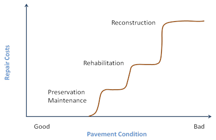
Figure 3. Graph. Conceptual relationship between agency repair costs as a function of pavement condition.
Under this scenario, the development of threshold limits is done through a combination of the approaches previously described. The recommended approach to setting threshold limits on need for corrective construction intervention is by using a combined engineering economic approach. The objective should be to determine condition states where maintenance or preservation treatments, rehabilitation treatments, and reconstructive treatments are most cost effective. Considerations to determine appropriate pavement state thresholds for application of maintenance or preservation treatments include the following:
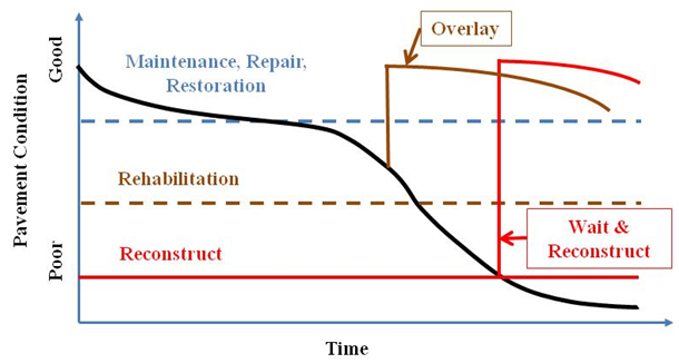
Figure 4. Graph. Three treatment zones as a function of pavement condition.
A common rule of thumb is that an overlay thicker than 2 inches (50 mm) is considered to be a structural improvement regardless of the depth of material milled from the pavement surface. Another common threshold rule used is that when the treatment cost rises to a certain level set by the agency, it is considered a capital improvement project and requires formal engineering plans and specifications. Like definitions of preservation maintenance, the definition of pavement rehabilitation is also dependent on available funding agency sources. The upper pavement condition threshold limit for rehabilitation is based on when preservation maintenance is no longer effective. Lower limit rehabilitation pavement condition thresholds are based on when reconstruction becomes the most cost effective treatment. There are also situations when structural defects may require reconstruction to correct even though all other functional aspects of the pavement are acceptable.
Expectancy performance curves are used as a means to predict the time when a pavement’s condition will reach a construction trigger threshold. While measuring the pavement condition can be used to respond to current conditions, long-term planning of future needs and optimization requires predicting future pavement changes.
A key consideration in developing performance curves is grouping pavement types into categories of pavement families. A pavement family is a group of pavement structures constructed with similar structural materials, construction methods, pavement components, and experience loading conditions and that are expected to have a common set of distress mechanisms. The number of pavement families that should be used depends on the diversity in types of pavement structures with an agency’s jurisdiction and the amount of time history data available for each defined family of pavements.
The best state-of-the-practice is to base performance expectancy curves on the analysis of pavement performance history observations. This requires the availability of uniform long-term time-series data on pavement condition that are linked to measured pavement features that permit the application of mechanistic-based performance models. When empirical data are not available to formulate proper statistical models of future performance, expected performance curves can be used as a surrogate starting point to judge the relative performance of pavements. For example, the knowledge of engineers with long-term experience in a region can be used as a surrogate starting point. While the use of expert subject opinion can be used as a starting point to create expectancy curves, the curves should be updated over time with field measurements to improve their accuracy and applicability. Potential expectancy curve options include models based on design equations, empirical models, and agency time-based rules.
Expectancy performance curves used for pavement design can be different than those used for pavement management. Nonetheless, they can be used for pavement management. Examples of models based on design equations include the following:
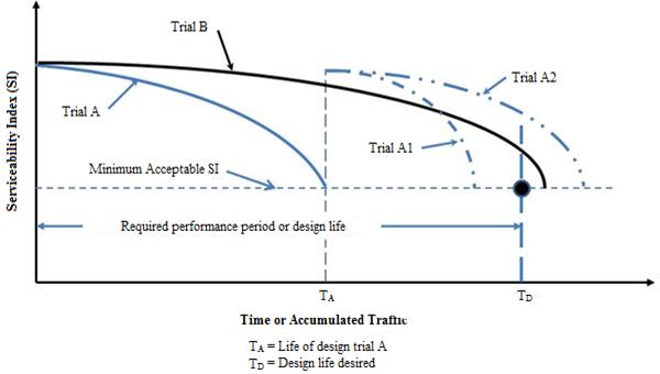
Figure 5. Graph. Illustrated service histories of trial pavement designs incorporating future overlays.(4)
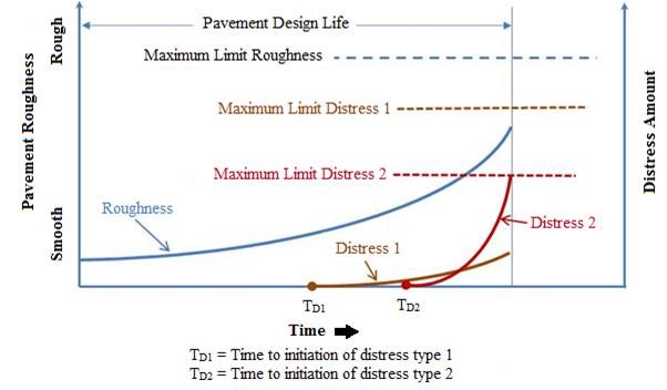
Figure 6. Graph. Multiple distress-based pavement design where one of the distresses reaches a maximum threshold limit.
These expectancy performance curves are based on observations of events. The following list summarizes empirical approaches to modeling pavement performance:
Some measure of variability distribution from function and relevant factors should be contained in all predictions of future pavement condition states. These measures can be used to accumulate future risk probabilities in the prediction based on the variability in the input parameters and prediction models.
The simplest future expectancy performance curve is a time-based rule for future construction. This type of rule does not require investing in field measurement devices and custom computer programs to predict future events. However, this approach does not provide a basis for optimizing utilization of constrained agency resources. An example of a time-based rule is that an agency decides that some type of corrective construction treatment will be applied on its rural interstates every 8 years. The network is segmented into contiguous projects, and a construction rotation sequence is established. An appropriate correction strategy is selected and applied during the target construction year. Thus, the expectancy curve for the time until the next construction event is the time remaining until the next target construction year.
Collecting data on the condition state of pavements under an agency’s jurisdiction should be based on the same construction triggers that form the basis for local decisions on corrective construction needs. Field data collection on current pavement conditions should properly be used to determine the impact of the data element on future construction requirements based on the current construction triggers. This effort is complicated with the need to adapt past and new pavement condition measurement practices.
The current challenge to SHAs is integrating, adapting, and adopting advancements in measurement of the physical features of pavement assets to legacy management systems. The development of datasets to establish expectancy curves of the long-term performance of a pavement requires a uniform set of data based on uniform measurements. Since common past pavement design practice was based on a 20-year life span, developing datasets with consistent data over this type of timeframe is difficult at best. This challenge will continue since emerging practice is to design some pavements with even longer lifetimes (i.e., 50 years).
The use of high-speed longitudinal pavement profile equipment has become the generally accepted industry standard for measuring pavement roughness. The measurement technique is based on using an inertial profiler, which measures the change in longitudinal profile in the wheel paths at or near the speed limit. Roughness indices are computed from this profile and summarized at user-defined intervals. IRI is one of the most commonly computed pavement roughness measures. Other pavement condition feature measures and indices can be computed from this type of profile data such as the roughness index, half-car roughness index, ride quality index, ride number (RN), profilograph index, rolling straight edge simulation, bump/dip detection, fault heights on jointed PCC pavements, slab curvature on jointed PCC pavements, and heavy truck dynamic loading index. If pavement roughness measurements are performed using inertial longitudinal profiler devices, as shown in figure 7, both network- and project-level data requirements can be satisfied using this common set of data.

Figure 7. Photo. Inertial road profilers used to measure IRI, RN, and other roughness indices.
Distress ratings can be performed by human raters driving on the pavement network using a manual process, a semi-automated process where field collected images are interpreted by human raters in an office, or fully automated systems. Manual pavement distress measurements require raters to drive each route and typically cost the most, put raters at risk (raters must drive and get down on the road to note any necessary information), and generally have the greatest variability in the ratings. In the semi-automated process, pavement distress ratings are performed using field video images, which reduce the risk to the raters and provide a historical archive of images for use in project-level investigations. Fully automated pavement distress ratings systems use computer algorithms to interpret distresses obtained from field images and/or three-dimensional measurements. It offers the potential to reduce the cost of acquiring distress data by eliminating the need for human interpretation. The newer three-dimensional imaging technology, which assigns a depth to image pixels, provides a more robust dataset that can be used for pavement cracking, rutting, and possibly pavement roughness measurements.
Deflection measurements are used to measure the response of a pavement structure to a known applied load. Interpretation of the resulting deflection data ranges from the identification of weak spots to advanced non-linear characterization of the engineering properties of pavement material layers.
Deflection measurement devices (e.g., falling weight deflectometers (FWDs) as shown in figure 8) currently used in practice must stop at each measurement location, which requires traffic control. To overcome traffic control requirements, agencies are in various stages of developing and implementing modern moving deflection measurement devices. The rolling wheel deflectometer can travel at highway speeds and does not require traffic control. While the maximum deflection measured by this device is useful in locating weak locations for follow-up studies, it does not provide additional analytical capabilities offered by devices that measure the shape of the deflection basin. The traffic speed deflectometer (TSD) is another type of moving deflection device that has sensors that measure the shape of the deflection basin (see figure 9 and figure 10).
To ensure accuracy of data interpretation using pavement deflection response devices, it is important to know the pavement thickness and types of near-surface material layers. Manual measurement techniques of pavement thickness are being replaced by automated ground penetration radar (GPR) technology. Pavement deflection measurements are mostly performed at the project level to develop design specifications for the most appropriate construction treatment. However, justification for network-level pavement deflection measurements can be based on the additional refinement in the decisionmaking process resulting from the ability provided by these data to determine the cost of future construction activities.

Figure 8. Photo. FWD used for structural evaluation.

Figure 9. Photo. TSD used for structural evaluation.
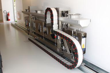
Figure 10. Photo. TSD internal pavement response measurement instrumentation.
For pavement management purposes, the preferred practice is to use weigh-in-motion (WIM) scales at non-enforcement locations to measure actual pavement loads as opposed to legally enforced loads. In order to accurately predict future pavement performance, engineers need to know actual heavy loads being applied to a pavement. Access to permitted overloads granted by other divisions within an SHA to the pavement management division could be important to determine the need for future construction intervention events.
At the network level, measuring the type of trucks on a route is more important than the weight of the trucks. This is based on the observation that truck weights are determined by the type of truck. This can simplify measuring heavy trucks into loaded and unloaded classes based on the simplest of WIM technology as shown in figure 11. Within a localized region, a typical heavy load truck profile can be applied to trucks in the same classification with an acceptable level of uncertainty. Project-level measurement of truck axle loads is almost never performed for pavement engineering purposes.

Figure 11. Photo. WIM sensor used to record truck axle and gross vehicle weights.
Climate data are at best a second-order consideration in the planning of future construction needs. Climate data measure potential climate-related “loads” such as freeze-thaw cycles and temperature-induced stresses that a pavement may need to resist based on material properties (as affected by climate) and constructed drainage features. Predicting future climate changes and accounting for is not currently incorporated in most pavement management models. The best source of historical raw climate data in the United States is available from the National Climate Data Center (NCDC). Figure 12 shows a mini seasonal monitoring program (SMP) weather station, which is an example of equipment used to collect climatic data.
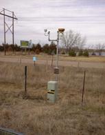
Figure 12. Photo. Mini site-specific SMP weather station used to record climatic data.
In addition to the data inputs themselves, it is also important to give serious consideration to the following data-related issues:
In order to select the most appropriate corrective pavement construction strategies, many considerations must be taken into account, beginning with the pavement condition subject to other constraints such as budget, bridge height clearance, guard rail adjustment, buried utilities, etc. At the pavement network level, the objective is to characterize the current and future condition state of pavements included in the system that require corrective treatments. At the project level, the objective is to provide detailed decisions on what corrective construction treatments are needed for each project identified from the network-level analysis.
The current challenge to highway agencies is to create a rational basis to move from a worst-first to a best-first (i.e., based on lowest LCC or other optimization technique) allocation of available agency repair resources. The application of corrective construction treatments at the proper time can extend the time until more costly treatments are required. These optimal treatments are applied before too much damage has accumulated and hence the pavements are not in the worst condition. To find these favorable pavement conditions at the optimum time requires knowledge of how a pavement will respond to the prescribed treatment plan based on its current condition.
There are also situations within a pavement network where pavements in a worse condition state should be allowed to continue to deteriorate. This type of decision is appropriate for pavements that have accumulated significant structural damage but are still smooth and provide adequate service otherwise.
The remainder of this section provides additional guidance concerning the network versus project analysis strategy selection process.
At the pavement network level, the objective is to characterize the current condition state of pavements included in the system that require the consideration of appropriate corrective treatments. Since network-level data tend to be more aggregated and less specific in comparison to project-level data, the expectancy models used to predict performance can have greater variability. Likewise, strategy selection may be broken down into broad categories using a standard set of cost assumptions based on the treatment type.
The recommended practice at the network level is to use LCC concepts to optimize the selection of construction projects in the next cycle and forecast future construction needs. LCC concepts consider multiple streams of future construction activities driven by predicting future changes in pavement states. Optimization is based on an objective function whose performance is based on measured field conditions and main factors that are sensitive to future construction activities. In a simple system, optimization is achieved when the best performance of the system is obtained using the available budget.
The pavement performance concept considers the time-history of a chosen functional aspect of a pavement. Serviceability has been used in the past using a scale - the lower the number, the worse the pavement condition. Using this type of scale, the objective function could maximize the area under of the serviceability-time history curve. If a numeric such as IRI is used, optimization of the objective function should focus on minimizing the area under the IRI-time curve since IRI uses an increasing scale where higher numbers indicate pavements in worse condition.
The limitations of construction strategy selection at the network level are based on the sophistication of the system processes. It is not uncommon that the construction cost assumptions used in the network optimization planning processes do not match those developed from project-level design considerations. Continual improvements are being made to field data collection techniques, construction cost models, and new expectancy prediction curves. Modern automated field data collection systems are capable of providing greater amounts of data with specificity that approaches what used to be considered project-level data. In order to use this increase in data availability from network-level measurements, updates to the sophistication of the construction triggers, threshold limits, and expectancy curves are required.
Strategy selection analyses at the network level are primarily based on computer algorithms capable of taking into account all of the factors included in the simulation of future pavement condition states and performing the millions of calculations for impact of alternative strategy scenarios needed for optimization of available budgets.
Project-level analysis is based on indepth considerations of pavement conditions after a network-level planning process has identified a pavement segment in need of corrective construction.The first level consideration determines the construction need as well as the maintenance, restoration, resurfacing, rehabilitation, or reconstruction needs. The most significant difference between network- and project-level strategy selection is that project-level decisions are based on human interpretations of available data and information as opposed to reliance on automated computer algorithms.
At the project level, LCC analysis can be supplemented with cost engineering considerations specific to each project site. Cost engineering concepts require more intensive inputs on the resulting effects of alternative design considerations than those generally available at the network level. This level of consideration is based on a cost/benefit analysis of alternative construction treatments based on a greater range of treatments options.
Project construction programming is the last chance to integrate other related infrastructure constructions needs into managing pavement assets. In urban areas, the timing of new utility cuts into a pavement structure should be coordinated with repaving events. Having a utility company perform changes to a pavement structure less than 3 years since the last construction event is often an indication of lack of coordination between publically funded city/regional departments. Studies on the impact of the repair of utility cuts in pavements have shown that they return the pavement to less than as new condition and can advance deterioration of the surrounding pavement structure.
Modern quality management system concepts are based on a continual cycle of assessments and updates. All systems require formal assessments. Based on the results of the assessments, updates are performed.
Regardless of the age of a management system, formal assessments should be performed at periodic intervals to identify improvement opportunities. Assessment tactics may include using panels composed of internal agency staff and external peer review experts. While internal review panels provide recommendations based on the current system, external peer reviews can provide lessons learned from the experience gained from use of other management methods.
As new materials and construction methods are implemented, the models used for both planning and designing need to be updated based on field observations. Creating a proper database designed to document past construction needs and planned construction needs is the recommended approach for updating the various elements included in the management system.