Estimation of Key PCC, Base, Subbase, and Pavement Engineering Properties From Routine Tests and Physical Characteristics

PDF Version (4.44 MB)

PDF files can be viewed with the Acrobat® Reader®

CHAPTER 5. MODEL DEVELOPMENT (13)

Elastic Modulus Model 2: Model Based on Age and Compressive Strength

The data used for validation were further reviewed to identify potential sources of error. Since the data covered a wide range of ages, the age parameter was considered for inclusion in the model. A model was developed to predict elastic modulus as a function of age and compressive strength at the corresponding age. The model was not entirely statistically optimized. The regressed constants were adjusted through a trial and error process to provide the best prediction (i.e., to match the measured with the predicted values as close as possible along the line of equality). The model can be expressed as follows:

Figure 194. Equation. Prediction model 10 for E_c,t.

Where:

E_c,t = Elastic modulus at age t years.

f'c_t = Compressive strength at age t years.

t = Age at which modulus is determined, years.

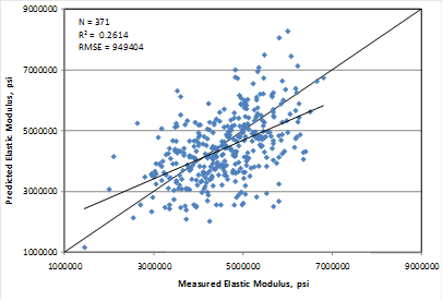
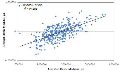
The model used 371 data points and had an R² value of 26.14 percent. The RMSE value for this model is about 900,000 psi. Table 41 shows the results of the nonlinear analysis, and table 42 provides details of the range of data used to develop the model. The measured versus predicted plot and the residuals plot for this model are shown in figure 195 and figure 196, respectively.

Table 41. Regression statistics for elastic modulus model based on age and compressive strength.

The model statistics for table 41 are as follows:

• RMSE = 949,404 psi.
• R² = 0.2614 percent.
• N = 371.

Table 42. Range of data used for elastic modulus model based on age and compressive strength.

Figure 195. Graph. Predicted versus measured for elastic modulus model based on age and compressive strength.

Figure 196. Graph. Residual errors for elastic modulus model based on age and compressive strength.

Elastic Modulus Model 3: Model Based on Age and 28-Day Compressive Strength

Since the 28-day compressive strength is usually available for PCC materials, a predictive model based on age and the 28-day compressive strength was developed. A relatively smaller dataset was utilized for this model with only data from SPS sections, as the 28-day compressive strength data was a necessary input. Again, this model utilized a nonlinear analysis, and beyond statistical optimization, the constants determined for this model were adjusted for closest predictions through a trial and error process. The relationship developed for these variables can be expressed as follows:

Figure 197. Equation. Prediction model 11 for E_c,t.

Where:

E_c,t = Elastic modulus at age t years.

f'c_28-day = 28-day compressive strength.

t = Age at which modulus is determined, years.

The model used 46 data points and had an R² value of 16.32 percent. The RMSE value for this model is about 1,183,400 psi. Table 43 shows the results of the nonlinear analysis, and table 44 provides details of the range of data used to develop the model. The measured versus predicted plot and the residuals plot for this model are shown in figure 198 and figure 199, respectively.

This model uses data up to an age of 1 year. It is more appropriate for estimating the short-term modulus of a project and for supplementing strength estimates used to determine opening time for traffic.

An examination of the statistics proposed for determining elastic modulus suggests that they do not possess the predictive ability of the other material parameters presented in this study. The models are considered fair but not excellent. They provide users with an option of moderate estimates when no information about the elastic modulus is available. It is therefore recommended that users exercise caution in using the predictive values for analyses.

Table 43. Regression statistics for elastic modulus model based on age and 28-day compressive strength.

The model statistics for table 43 are as follows:

• RMSE = 1,183,400 psi.
• R² = 0.1632 percent.
• N = 46.

Table 44. Range of data used for elastic modulus model based on age and 28-day compressive strength.

Figure 198. Graph. Predicted versus measured for elastic modulus model based on age and 28-day compressive strength.

Figure 199. Graph. Residual errors for elastic modulus model based on age and 28-day compressive strength.