U.S. Department of Transportation
Federal Highway Administration
1200 New Jersey Avenue, SE
Washington, DC 20590
202-366-4000
Federal Highway Administration Research and Technology
Coordinating, Developing, and Delivering Highway Transportation Innovations
| REPORT |
| This report is an archived publication and may contain dated technical, contact, and link information |
|
| Publication Number: FHWA-HRT-12-068 Date: December 2012 |
Publication Number: FHWA-HRT-12-068 Date: December 2012 |
Analyses were performed to segregate and quantify the portion of roughness caused by slab curl and warp within a profile and the portion associated with other sources of roughness such as built-in defects and surface distress.
The level of curl and warp present within each profile was estimated using slab-by-slab analysis of local profile segments. The automated procedure described in appendix D isolated the profile of each slab by seeking the locations where negative spikes appeared repeatedly in the same locations. The procedure described in this chapter quantifies the level of curl and warp on each slab using PSG, which is the gross strain gradient required to deform a slab into the shape that appears within its measured profile from a flat baseline.
Using PSG to quantify curl and warp represents an approach similar to the calculation of equivalent temperature gradient from measured slab profiles.(19, 20) PSG is used rather than equivalent temperature gradient because this study sought to relate curl and warp to IRI rather than relate content within the profile to the environment in which the pavement functions.
Other examples of this analytical strategy for processing slab profiles have been documented by Sixbey and Vandenbossche.(21, 22) Those studies applied curve fitting to profiles of individual slabs using appropriately selected polynomials to represent idealized slabs with a strain gradient. The specific approach applied in this study uses an idealized profile for a slab with curling and warping proposed by Westergaard in the classical literature.(23) With only minor exceptions, the step-by-step procedure used in this study follows the analysis methods proposed by Rasmussen and applied by Chang.(2, 24) Portions of this appendix duplicate the descriptions by Chang, with additional specific information pertinent to this study.(2, 24)
The curve fitting procedure for measured slab profiles used an idealized shape proposed by Westergaard.(23) The idealized profile is based on the assumption of a linear temperature and moisture gradient through the depth of the slab, unrestrained slab ends, and an infinite slab along the undeformed axis. Westergaard provided the solution for an infinitely long pavement of finite width. This study applies the solution to an infinitely wide slab of finite length.
The idealized profile relates the slab elevation (z) to position along the slab as shown in figure 72.
 |
| Figure 72. Equation. Relationship of Slab Elevation to Position. |
Where:
x is the horizontal coordinate along the slab profile, referenced to the slab center (L).
z0 is the uplift at the slab ends (L).
l is the radius of relative stiffness (L).
b is the slab width (used as slab length here) (L).
E is slab elastic modulus (F/L2).
μ is Poisson’s ratio (–).
k is the modulus of subgrade support (F/L2/L).
Figure 72 is a specialized version of the Westergaard solution that includes both moisture gradient (Δεsh/h) and temperature gradient (αΔT/h).
The four independent pavement properties b, E, μ, and k are parametric inputs needed to estimate l. The curve fitting procedure applied in this study assumes a fixed value for the five aforementioned parameters along a pavement section and seeks the optimal value for total strain gradient on each slab segment as shown in figure 73.
| Figure 73. Equation. PSG |
PSG is given the prefix “pseudo” because it is estimated empirically.
The PSG associated with each slab profile was estimated using the following procedure.
Crop the profile of the slab to exclude the negative spikes at the joints. Appendix E describes the procedure for determining the location of the joints. Set the profile starting point to the end of the spike group found at the leading joint plus a small offset. Set the profile ending point to the start of the spike group found at the trailing joint minus a small offset. This study applied an offset of 1 inch.
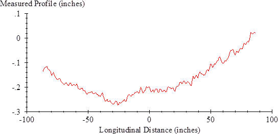
Shift the longitudinal scale to place the slab center at a value of 0. Assume that the center of the slab is at the midpoint between the two average spike position values, derived as described in appendix E. Figure 74 shows an isolated slab profile after offset of the longitudinal scale.
 |
| Figure 74. Graph. Measured Slab Profile for Section 0215. |
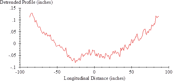
Detrend the isolated profile. Apply a least-squares linear fit to the profile segment and subtract the best-fit line point by point. The resulting signal will have a zero mean. Figure 75 shows the detrended profile.
 |
| Figure 75. Graph. Detrended Slab Profile for Section 0215. |
Estimate the pavement properties needed to apply the Westergaard equation for the slab under examination. The LTPP database includes measurements of elastic modulus (E), Poisson’s ratio (μ), and slab thickness (h) for each section. For this study, these values were held constant for all slabs within a given section. Values for modulus of subgrade support (k) were not available, and a value of 200 psi/inch was used for the entire experiment. Table 32 lists the values of E, μ, and h for each section, as well as the radius of relative stiffness (l).
The joint-finding procedure provided the length of each slab (b). To obtain slab length, calculate the longitudinal distance between the average spike positions at the leading and trailing joint. Each slab requires a distinct estimate.
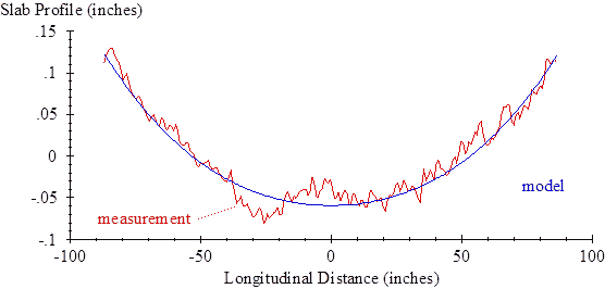
Perform a non-linear curve fit of the Westergaard model to the measured slab profile. This provides an estimate of the PSG required to optimize the linear fit. In this study, curve fitting was performed using functions MRQMIN and MRQCOF provided in Numerical Recipes.(25)
Figure 76 shows a sample curve fit for a slab on section 0215. For this slab, the routine used a slab length of 15.1 ft and radius of relative stiffness of 40.7 inches. For this slab, the routine returned a PSG value of 70.57 × 10⁻⁶ in units of strain per inch or 70.57 με/inch.
 |
| Figure 76. Graph. Curve Fit for Section 0215. |
Summary PSG values for a section were compiled using a weighted average of the absolute slab-by-slab PSG values. A weighting factor was applied to the PSG values in proportion to their length, relative to the overall section length. For slabs that appeared at the ends of a section, a weighting factor was applied to the PSG values in proportion to the length that appeared within the section, relative to the overall section length.